A novel quantitative analysis for diurnal dynamics of Ulva prolifera patch in the Yellow Sea from Geostationary Ocean Color Imager observation

1 Introduction

“Green tides” is a phrase typically used to refer to an ecological disaster caused by the excessive proliferation, growth, and aggregation of large green algae in seawater under certain environmental conditions (Valiela et al., 1997; Liu et al., 2013). Green tides events began in the 1960s and 1970s, and frequently broke out on a large scale in the coastal waters of many countries. These events have become a worldwide problem for the marine ecological environment (Ye et al., 2011; Smetacek and Zingone, 2013). Since 2007, green tides with Ulva prolifera as the main cause have broken out periodically in the Yellow Sea from May to July every year, which has seriously affected the ecological environment of the region, causing serious social impacts and very high economic losses (Ye et al., 2011; Zhou et al., 2015). The Yellow Sea green tides of Ulva prolifera are considered the largest-scale green tides in the world and have become the most serious ecological disaster in the local area (Zhou et al., 2015; Yu and Liu, 2016). Therefore, timely, accurate, and effective access to green tides information is essential for monitoring, managing, and preventing this type of marine disaster. Green tides disaster events have the characteristics of fast drifting speed and wide distribution. Satellite remote sensing techniques can provide continuous observation data on temporal and spatial scales to accurately capture the time, extent, and area of Ulva prolifera outbreaks in real time. These techniques have irreplaceable advantages over traditional survey and measurement methods; in particular, optical remote sensing satellites have been frequently used to monitor green tides (Qi et al., 2017).

Based on the optical characteristics of Ulva prolifera, green tides monitoring methods and case studies have been widely reported with the development of remote sensing satellite techniques. According to the “redshift” characteristic of Ulva prolifera at around 700 nm (Hu and He, 2008), many remote sensing monitoring algorithms have been proposed, such as the single-band threshold method, the multiband ratio method, and the supervised classification method. For example, Shi and Wang (2009) proposed the normalized difference algae index (NDAI) green tides detection algorithm for moderate resolution imaging spectroradiometer (MODIS) data. Although the calculated NDAI value is easily affected by atmospheric conditions, the algorithm can discriminate green tides and seawater information after AC better than traditional algorithms. Hu (2009) established a green tides remote sensing monitoring method based on the floating algal index (FAI). Compared with other traditional remote sensing monitoring algorithms, the FAI method showed higher stability and was more suitable for green tides detection under various environmental conditions. In addition, Shanmugam et al. (2013) proposed an ocean surface algal bloom index (OSABI) that can more accurately quantify the algal bloom coverage area, and this method can be used to more easily distinguish the algal bloom outbreak stage. Xing and Hu (2016) developed the virtual baseline index of floating algae height (VB-FAH) for the HJ-1 satellite and analyzed the green tides outbreak in the Yellow Sea.

Compared with polar-orbiting satellites, the advent of geostationary satellites has opened up a new research direction for green tides detection. The Communication Ocean and Meteorological Satellite (COMS), the world’s first geostationary ocean color satellite equipped with GOCI, was launched by Korea in June 2010 (Amin et al., 2015). The high-frequency ocean color data of northeast Asia that it produces have been successfully applied to the remote sensing monitoring of green tides in the observed sea areas. The index of floating green algae for the GOCI (IGAG) is measured by using an algal extraction algorithm based on field measurements and GOCI data (Son et al., 2012) and has been applied to Ulva prolifera disaster monitoring. The results of selected cases showed that the accuracy of the IGAG algorithm was higher than that of the NDVI and enhanced vegetation index (EVI). Using GOCI data and Lagrangian particle tracking experiments, Son et al. (2015) presented the movement path of floating green algae patches and explained the physical forcing factors that affect algae drift and distribution. The high temporal resolution of the GOCI sensor can also realize the diurnal variation monitoring of floating algal blooms. Lou and Hu (2014) established an improved red tide index (RI) using GOCI data and proved that the index can effectively describe the bloom of Prorocentrum donghaiense. They also found that red tide blooms evolved during the day, their physical location was driven by tides, and vertical migration of Prorocentrum may be the main reason for the area change during the day. Song et al. (2018) used high temporal resolution GOCI remote sensing imagery to extract information on Ulva prolifera in the South Yellow Sea in 2017 and analyzed the evolution characteristics. The diurnal variation in the Ulva prolifera coverage area tended to increase and then decrease. Based on the band characteristics of the GOCI sensor, Chen et al. (2020) designed a new green tides index algorithm based on the tasseled cap transformation method. They proved that the new method has high reliabilityand also explained that the monitored green tides coverage area reached a maximum expansion at noon, which may be affected by photosynthesis.

Related studies have shown that the accuracy of GOCI products obtained at noon is higher than that in the morning and evening, and the deviation of data in bands 5 to 8 is larger than that at noon (Lamquin et al., 2012; Moon et al., 2012; Qiao et al., 2021). On the one hand, the weak light during the twilight periods increases the difficulty of AC and inhibits the collection of water color information; on the other hand, the large solar zenith angle and the observation zenith angle reduce the ability of the water color satellite to detect chlorophyll (Concha et al., 2019; Li H et al., 2019; Li et al., 2018). In addition, under the large solar zenith angle in the twilight periods, due to the influence of the large solar zenith angle and the curvature of the earth, there is also a certain error in the Rayleigh-corrected reflectivity calculated by the standard AC algorithm (Gordon et al., 1988; Wang, 2002; He et al., 2018). Therefore, the vegetation index method based on band combination is affected by the deviation of band reflectance during twilight when extracting green tides information. Furthermore, the change in the solar zenith angle during the day causes a change in the vegetation index value. The green tides data extracted by the vegetation index consist of pixel information with a wide range distribution, while the Ulva prolifera in the Yellow Sea is mainly distributed in stripes and large patches in the flourishing period (Qiao et al., 2009). Due to its unique distribution characteristics, the clustering method has certain advantages for the overall data extraction of single patches. Density based spatial clustering of applications with noise (DBSCAN) is a density-based clustering algorithm (Wishert, 1969; Hartigan and Wong, 1979; Ester et al., 1996). Because of its good performance and robustness, it has been widely used in outlier detection (Hu et al., 2014), image segmentation (Shi and Ma, 2018), data compression (Manavalan and Thangavel, 2011), and other applications. Ji and Zhao (2015) used the spatiotemporal trajectory adjoint pattern mining method based on the DBSCAN algorithm to extract useful information from massive spatiotemporal trajectory data and provide decision support for smart cities. Çelik et al. (2011) used the DBSCAN algorithm to process annual temperature data and identified the temperature law and abnormal temperature. Using the method of combining the DBSCAN algorithm with the gray method (Ju-Long, 1982), Jiang and Zhang (2017) analyzed the trajectory of hurricanes based on the structural distance, which provided a reference for weather forecasting and other applications. To identify the characteristics of mesoscale vortex detection in sea level anomaly (SLA) data, Li J et al. (2019) proposed a new mesoscale vortex automatic identification algorithm based on the density clustering method. The algorithm not only has an improved efficiency compared with the traditional algorithm but also maintains high stability. It can identify each single vortex structure while also identifying stable multivortex structures. The above research proves that the DBSCAN method can be applied to not only land fields but also the detection of marine environments.

Therefore, considering the high temporal resolution of the GOCI sensor and the patchy distribution of floating Ulva prolifera in the Yellow Sea, we proposed a method of Ulva prolifera extraction based on DBSCAN clustering analysis. Based on the extraction of Ulva prolifera information by the NDVI algorithm, the DBSCAN method for clustering analysis was used to quantitatively analyze the drifting path of a single Ulva prolifera patch and its driving mechanism, as well as the diurnal variation characteristics of the coverage area.

2 Materials and methods

2.1 Satellite data processing

The GOCI L1-B data can be downloaded from the Korea Ocean Satellite Center (KOSC) website (http://kosc.kiost.ac.kr), covering 8 bands of visible light and infrared light from 412-865 nm. The satellite can perform hourly observations from 8:30 to 15:30 (Beijing time, all times in this paper are Beijing time). The advantages of spatial resolution (500 m) and temporal resolution (1 h) can be used to monitor the offshore marine dynamic environment. Through data screening of pseudo-color RGB images, it was found that the study area had minimal cloud instances cover on 26 May 2012 and 27 May 2017, and eight valid images were obtained. Both were in the flourishing period of green tides development at the same time and therefore were selected as research objects. GOCI provides multilevel data products, and L2 data products for marine environmental factor analysis can be further obtained by processing L1-B data (Wang et al., 2017). In this study, GOCI-L2C data corrected by Rayleigh scattering were selected for remote sensing monitoring and extraction of Ulva prolifera in the Yellow Sea. Using GOCI Data Processing Software (GDPS) with default parameters and standard AC, Level-1B data was processed into Level-2 data to obtain spectral Rayleigh-corrected reflectance (Rrc) products after gas absorption correction, sea white hat correction, and Rayleigh correction (Ryu and Ishizaka, 2012). The GOCI standard AC algorithm is based on the Sea-viewing Wide Field-of-view Sensor (SeaWiFS) standard AC algorithm (Wang and Gordon, 1994), with enhancements made to account for multiple scattering effects and improved in terms of turbid case-2 water correction, optimized aerosol models, and solar angle correction per slot. Among them, for turbid water correction, the regional empirical relationship between the water reflectance of the red (660 nm) and the near infrared bands (745 nm and 865 nm) was used (Ahn et al., 2012). The specific procedure is as follows: The atmospheric transparency of the preprocessed GOCI data is estimated by calculating the ratio between different bands, with the blue and green band (412 nm and 555 nm) typically serving as reference. Subsequently, the built-in atmospheric scattering model is employed to correct the data based on the estimated atmospheric transparency. According to the Rayleigh scattering model and the estimated atmospheric transparency, the corrected data are corrected by Rayleigh scattering. After the atmospheric and Rayleigh scattering correction, combined with the predefined atmospheric model, considering the influence of water characteristics and atmospheric scattering, the reflectivity of water can be calculated. Finally, by utilizing the established ocean optical algorithm and applying the corrected water reflectance, one can obtain the corresponding ocean parameter products. Furthermore, the corresponding high spatial resolution Landsat_8 Operational Land Imager (Landsat_8/OLI) image data (30 m resolution) were downloaded from the geospatial data cloud (https://www.gscloud.cn/sources/accessdata/411?pid=263). Radiance calibration and Fast line – of fight atmospheric analysis of spectral hypercubes (FLAASH) AC (Matthew et al., 2003) were performed using ENVI, and the RGB image was output by pseudo-color synthesis for validation with GOCI recognition results.

2.2 Research area and tidal data

This paper takes the Yellow Sea as the study area (Figure 1). Affected by semidiurnal tides, there are approximately two flood tides and two ebb tides in the study area every day (Hsueh, 1988; Teague et al., 1998). The tidal current is one of the important local hydrodynamic processes. The hourly tidal height data of two tidal stations, point A and point B, near the study area are collected from the local tide tables released by the National Marine Data Center (NMDC), National Science & Technology Resource Sharing Service Platform of China(http://mds.nmdis.org.cn/) (Figure 1). Tidal height and tidal current data can also be calculated by using ocean models. TPXO-CSI2016 (China Seas & Indonesia 2016) is a regional tidal model in the China seas established by Oregon State University (OSU) (Egbert et al., 1994; Egbert and Erofeeva, 2002). The model is based on the Laplace tidal equation, uses the least squares method, and assimilates large amounts of satellite altimeter data and measured site data, with a spatial resolution of 1/30° (http://www.tpxo.net). The Tidal Model Driver (TMD) (https://www.esr.org/research/polar-tide-models/tmd-software) is used to run the OSU tidal current model for tidal prediction and tidal current calculation in designated areas (Padman and Erofeeva, 2005). Using the tidal current model, the tidal current data at the same observation time as the GOCI (setting the output resolution to 0.1° × 0.1°) and the corresponding tidal height data are extracted.

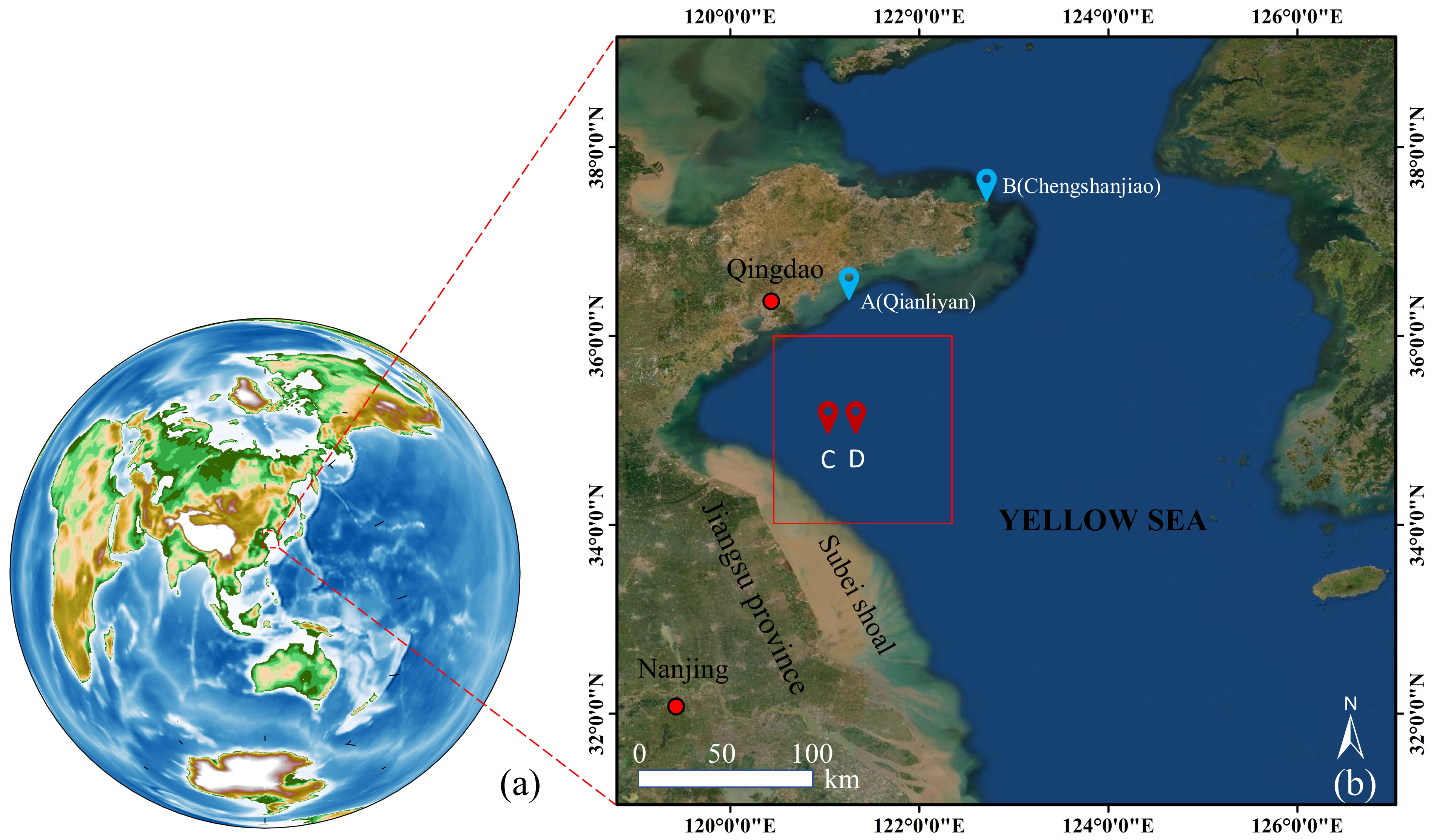
Figure 1 Satellite image of the Yellow Sea. In (B), the red box is the study area, blue points A and B are the two nearby tide stations, and red points C and D are the locations selected to obtain the tide height information in the study area.

2.3 Ulva prolifera extraction method based on DBSCAN clustering analysis

Similar to the spectral reflectance characteristics of terrestrial plants, Ulva prolifera has low reflectance in the visible band and high reflectance in the near-infrared band, and the spectral difference between Ulva prolifera and water is obvious (Hu et al., 2010). Therefore, as a quantitative algorithm based on band operation, the vegetation index has become the mainstream algorithm for Ulva prolifera remote sensing detection. Previous studies have shown that NDVI has a more prominent detection ability than other vegetation index algorithms and can still be used as the preferred algorithm for satellite green tides operational monitoring (Cai et al., 2014; Song et al., 2018). For GOCI data, the band selection of the 5th (660 nm) and 7th (745 nm) bands for the vegetation index calculation has better stability (Song et al., 2018). Therefore, the combination of the 5th and 7th bands in the NDVI algorithm was used as the Ulva prolifera detection algorithm in this study, as follows:

After the NDVI calculation of the GOCI data, it is necessary to use image segmentation technology to separate the Ulva prolifera information from other information, such as seawater information, for the next step of clustering. As one of the traditional image segmentation methods (Otsu, 1979), the basic principle of the threshold method is to set different thresholds and divide the pixels of the image into several categories. If the original image is F(x,y), the eigenvalue T is found in F(x,y) according to certain criteria and applied to image segmentation. The segmented image is:

If a₀ = 0 (black pixels) and a₁ = 1 (white pixels), this is the binarization of the image (Sezgin and Sankur, 2004). In this study, we select the threshold segmentation method for image binarization.

The DBSCAN algorithm can perform clustering analysis by the closeness of the sample distribution and can effectively screen outliers. The NDVI algorithm combined with DBSCAN clustering analysis can perform the extraction of a single Ulva prolifera patch (Figure 2). According to the set radius Eps and the number of samples MinPts, the DBSCAN algorithm divides the data to be clustered into three categories: core points, boundary points, and noise points. Among them, the points that contain at least MinPts samples in the circle with radius Eps are called core points. The points that do not belong to the core point but are in the neighborhood of a core point are called boundary points. Those that are neither boundary points nor core points are called noise points. The cluster center to which each sample belongs is determined by defining direct density reachability and density connectivity. Direct density reachability means that for a given radius Eps and sample number MinPts, it is necessary to directly reach sample Q from sample P:

Figure 2 Technique flow chart.

where NEps(q) is the sample range of sample Q. Density connected means that there are samples that satisfy P and Q are density reachable for both Eps and MinPts. The specific DBSCAN clustering algorithm is as follows: і) Set the dataset D, the radius Eps, and the number of samples MinPts; ii) Determine if the input sample points are core points; iii) If the input sample is a core point, determine all direct density accessible points in its neighborhood; iv) Repeat steps ii) and iii) until all samples are evaluated; v) Merge some density accessible objects, and find the set of connected points with maximum density according to the direct density accessible points in the neighborhood of all core points; vi) Repeat step v) until all core point neighborhoods have been traversed.

There are very tiny patches (the red crosses in Figure 3 represent outliers or noise) around the large area of Ulva prolifera extracted by the NDVI algorithm. Including them in the calculation causes errors in the statistical area, so they are deleted. The DBSCAN algorithm is used to process the image results after NDVI extraction and binarization, which can not only cluster large-area algae but also screen out sporadically distributed tiny patches and eliminate the errors caused by area statistics. In this study, the DBSCAN function developed in the MATLAB statistics and machine learning toolbox was used to realize the clustering of Ulva prolifera. The function contains two important parameter values: Eps and MinPts, which correspond to the radius and the number of samples in the DBSCAN algorithm, respectively. Among them, too large Eps lead to fewer classification types, and too large MinPts lead to more outliers. Therefore, the selection of two parameter values follows the following principles: combined with the method of visual interpretation, according to the extraction results of the GOCI pseudo-color image and NDVI extraction and binarization, the number of classifications of Ulva prolifera after clustering was roughly counted, and the initial values of two parameter values were selected according to the number of classifications. As shown in Figure 4K, according to the aggregation degree of Ulva prolifera patches, the six main parts were selected and classified (red ellipse marker) by visual interpretation. Then, according to the classification of large patches after visual interpretation, the number of outliers was minimized, and the two parameter values were appropriately adjusted to obtain the best clustering results. As shown in Figure 4O, the large patches marked by red ellipses have achieved ideal clustering results. Table 1 shows the Eps and MinPts values set by clustering analysis at each time of the study case. Ulva prolifera algae in the floating process, affected by the surrounding environment, produces edge algae separation phenomena. To eliminate the area error caused by algae separation, according to any banded or patchy algae after clustering, this study took the algae with the largest distribution area of the day as a reference to count the coverage area of algae at other times. Among them, the distribution area is the total area within the envelope of the same class of algae after clustering analysis; the coverage area is the actual coverage area of floating Ulva prolifera, and the area statistics involved in this study are the coverage area.

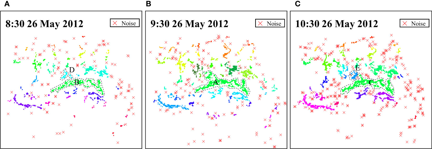
Figure 3 Diagram of algae clustering combined with visual interpretation. (A–C) represent the clustering results of three adjacent times of 8:30-10:30, and the red crosses are the selected sporadic algae, representing the outliers. Patch A is the algal body with the largest distribution area on that day, patch B and patch C are the algal bodies extracted at the corresponding time before and after, and patch D and patch E are the algal bodies that are different from patch B and patch C, respectively.

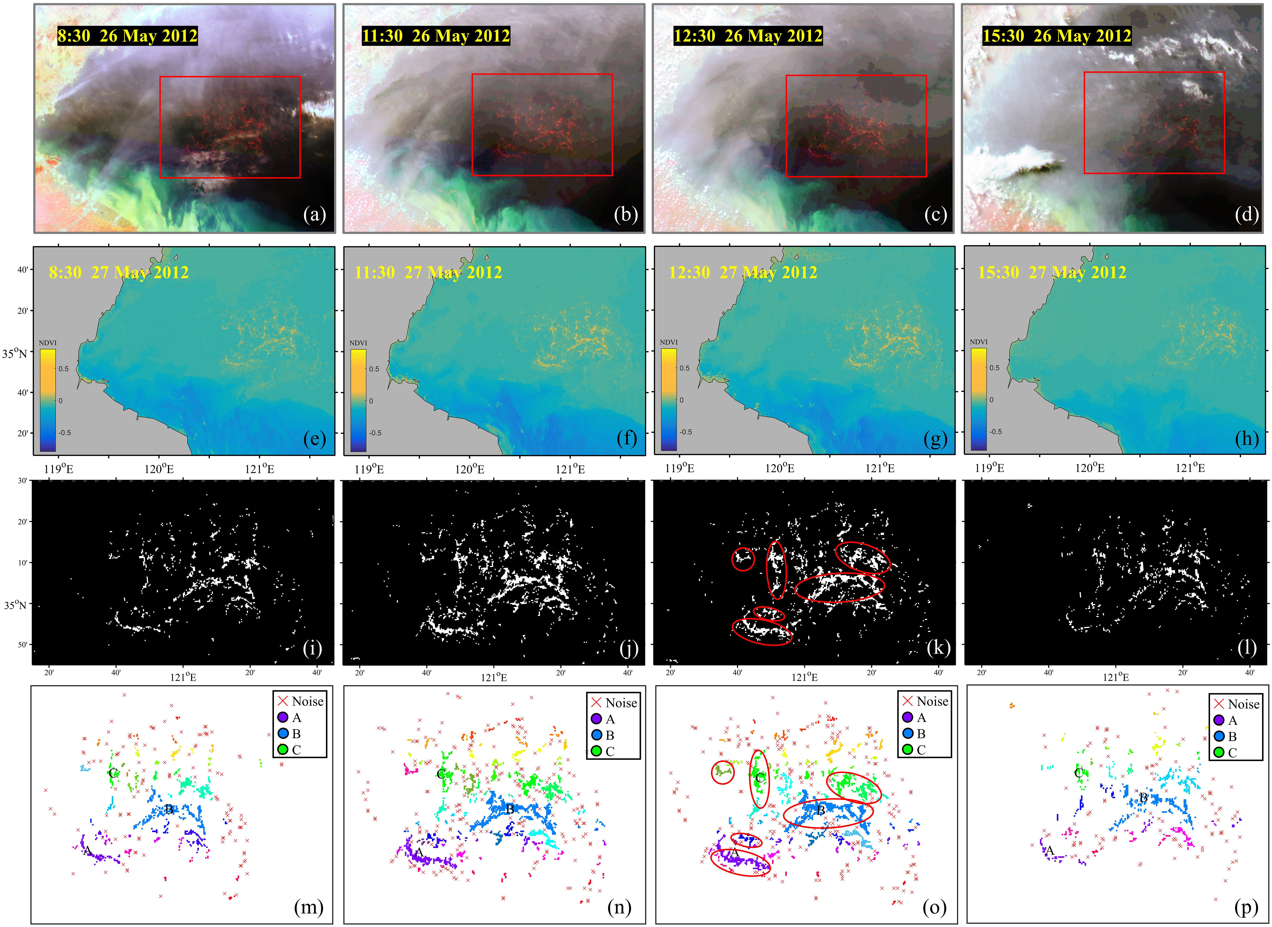
Figure 4 Extraction results of Ulva prolifera at four time points on 26 May 2012 (8:30, 11:30, 12:30, and 15:30). (A–D) represent the pseudo-color images of the four time points, and the detected Ulva prolifera is outlined in red. (E–H) represent the NDVI extraction results. (I–L) represent the binarization results after threshold segmentation; (M–P) represent the DBSCAN clustering results, and single Ulva prolifera patches were selected for diurnal variation analysis.

Table 1 Eps value and MinPts value set by DBSCAN clustering at each time.

2.4 Case study

The selection of parameters and the algae separation phenomena in the clustering analysis in Section 2.3 will be explained by a case. Figure 3B shows the clustering analysis result of Ulva prolifera algae at 9:30 on 26 May 2012. When Eps = 2 and MinPts = 3, the classification result is the most obvious, and the outliers are the least, which is the best clustering result. The explanation of algae separation is shown in Figure 3. Patch A is the largest algae in the distribution area of the day, and patch B and patch C are the corresponding algae extracted at the time before and after, respectively. According to the clustering results, patch D and patch E are different from patch B and patch C, respectively. However, referring to the clustering results of patch A, it can be identified as the edge algae separation phenomena. In the area statistics of patch B and patch C, patch D and patch E still need to be counted.

3 Results

3.1 Extraction results of Ulva prolifera

In this study, the NDVI green tides extraction algorithm combined with visual interpretation and the DBSCAN clustering method was used to extract Ulva prolifera from preprocessed GOCI_Rrc data of the study area. The results for 8:30, 11:30, 12:30, and 15:30 were selected for display (corresponding to two morning and afternoon times and two noon times, respectively). Figure 4 shows the result of clustering analysis after extraction of Ulva prolifera on 26 May 2012. The pseudo-color images were derived from the GOCI_Rrc data, with the detected Ulva prolifera in the red box (Figures 4A–D). The yellow highlighted area in the NDVI extraction results is the area where Ulva prolifera is heavily aggregated with high NDVI values (Figures 4E–H). The area extracted at noon is larger than that extracted in the morning and afternoon. Further threshold segmentation is performed, and the threshold setting is mainly determined by observing the distribution of Ulva prolifera in pseudo-color images and the extraction results of NDVI. The threshold on 26 May 2012 is set to 0. The threshold segmentation results show that Ulva prolifera has a banded or patchy distribution (Figures 4I–L). Figures 4M–P shows the results of clustering by the DBSCAN method. The algal bodies gathered in different patches or bands were divided into different colors, and sporadic algal bodies were screened out as noise, which well realized the extraction of a single algal body. Figure 5 shows the extraction results on 27 May 2017. In addition, the threshold segmentation threshold is set to 0 (Figures 5I–L), and the remaining observation results and NDVI extraction results are similar to those on 26 May 2012. To further analyze the diurnal variation characteristics of a single Ulva prolifera patch, three patches, patch A, patch B, and patch C, were evenly selected from the two-day extraction results for further study.

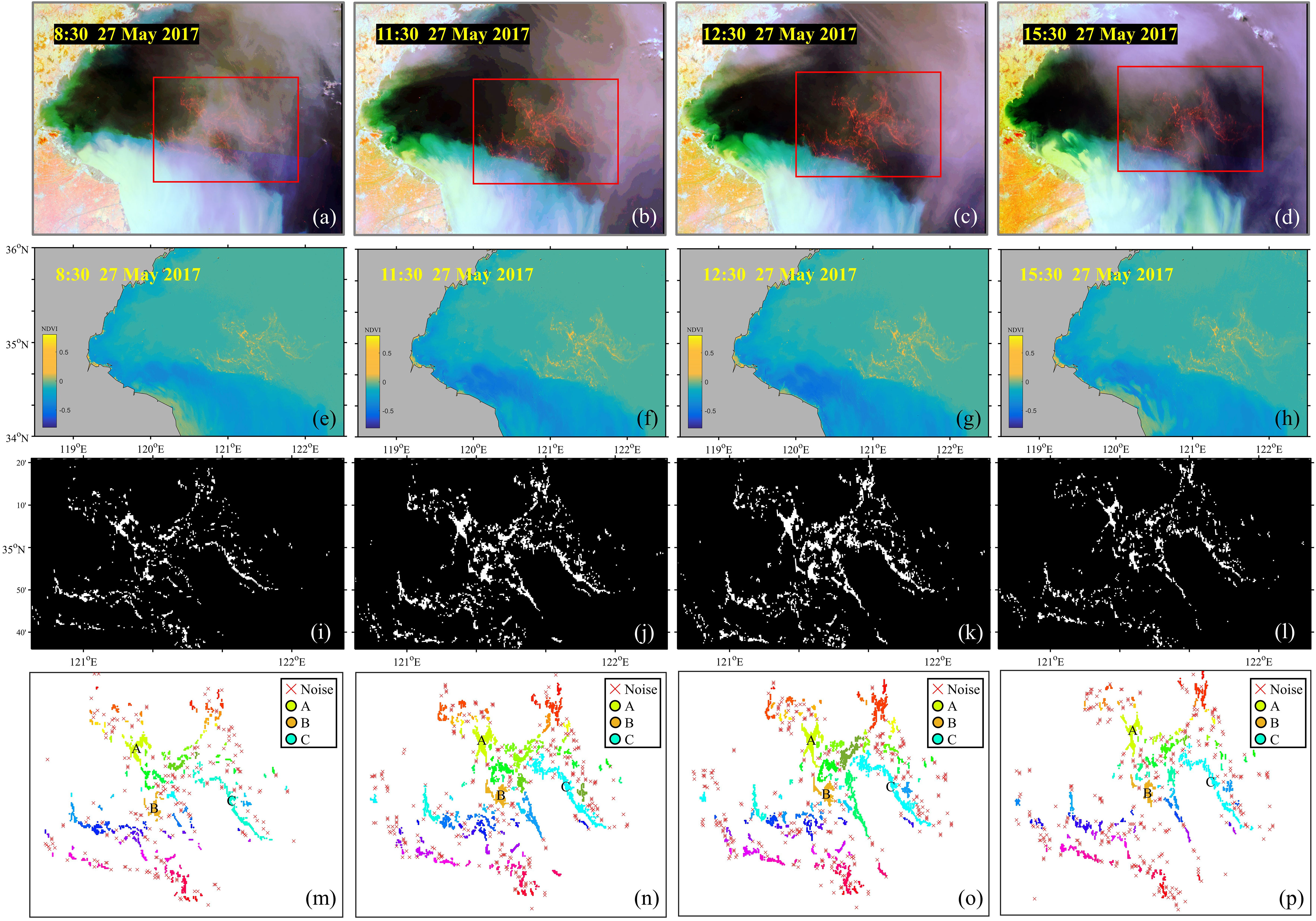
Figure 5 Extraction results of Ulva prolifera at four time points on 27 May 2017 (8:30, 11:30, 12:30, and 15:30). (A–D) represent the pseudo-color images of the four time points, and the detected Ulva prolifera is outlined in red. (E–H) represent the NDVI extraction results. (I–L) represent the binarization results after threshold segmentation; (M–P) represent the DBSCAN clustering results, and single Ulva prolifera patches were selected for diurnal variation analysis.

Figure 6 shows the verification of the GOCI recognition results for the higher resolution Landsat_8/OLI image. The Landsat_8/OLI image of the study area at 10:30 on 27 May 2017 is selected for preprocessing (Figure 6A), and the red box is the detected Ulva prolifera (corresponding to Figure 6B). It is compared with the NDVI extraction results of GOCI (Figure 6C) and DBSCAN clustering results (Figure 6D). Although the NDVI extraction results of GOCI data are not sufficiently refined, they can still reflect the morphological characteristics of Ulva prolifera patches, which can realize the extraction and identification of a single patch and meet the research needs of this paper.

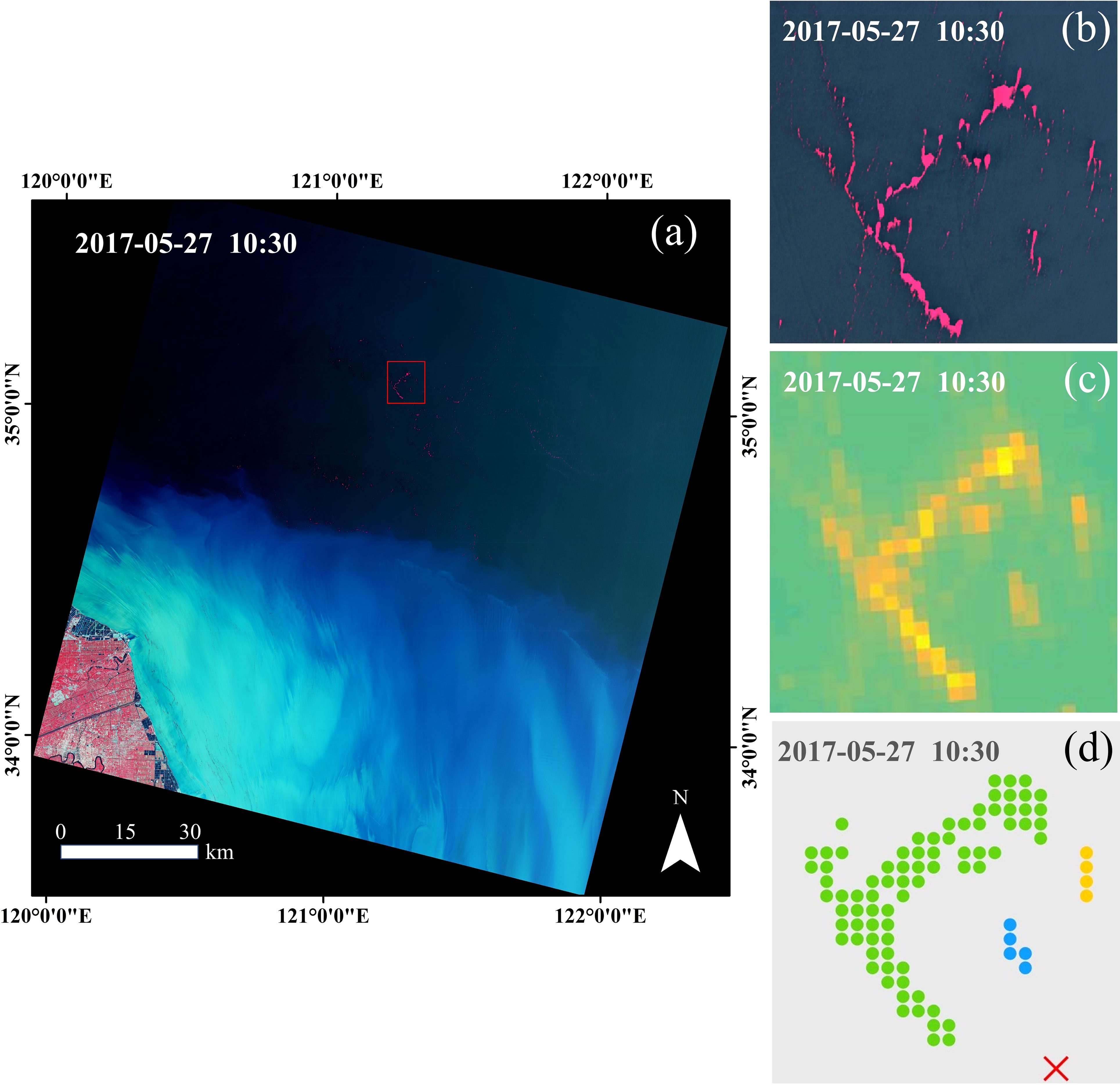
Figure 6 Verification of GOCI recognition results by Landsat_8/OLI. (A) Shows the Landsat_8/OLI remote sensing image of the pre-processed study area. (B) Distribution of part of Ulva prolifera selected by the red box in (A). (C) Shows the NDVI extraction results corresponding to GOCI data. (D) Shows the result of DBSCAN clustering analysis.

3.2 Diurnal variation characteristics

3.2.1 Drifting path and driving mechanism

Field observations from the historically moored acoustic Doppler current profiler (ADCP) and drifting buoy have verified the OSU tidal current data in the Chinese seas. The average magnitude error between the total surface currents (including tidal currents and wind-driven currents) obtained by the ADCP and the OSU outputs is approximately 0.5 cm/s, and the average angle error is 10° (Jiang and Wang, 2016). The measured currents obtained by the drifting buoy are highly consistent with the OSU outputs in the direction of currents and rotation (Cui et al., 2022). These findings indicate that tidal currents are dominant, and wind-driven velocities play an extremely limited role in the total surface currents in the Chinese seas (Lie et al., 2002; Hu et al., 2016). Therefore, we compared the tidal current direction output by OSU with the drifting direction of Ulva prolifera and analyzed the driving mechanism of Ulva prolifera within one day. Figure 7 shows the hourly drifting path of the three Ulva prolifera patches A, B, and C within one day. The background blue vector is the tidal current result output by OSU. The form is the superposition of the tidal current results in all periods from 8:30 to 15:30. The drifting direction of Ulva prolifera is basically consistent with the local tidal current direction. Figure 7A shows the drifting path of Ulva prolifera extracted on 26 May 2012, and its drifting direction and tidal current direction are both eastward. Figure 7B shows the drifting path of Ulva prolifera extracted on 27 May 2017. Ulva prolifera first moved northeast, then turned to the north, and finally slightly deviated to the northwest. However, the overall direction within a day is northeast, consistent with the direction of the tidal current. Figures 7C, D show the drifting direction of Ulva prolifera in 2 or 3 adjacent periods in the case, which is basically consistent with the corresponding tidal current directions.

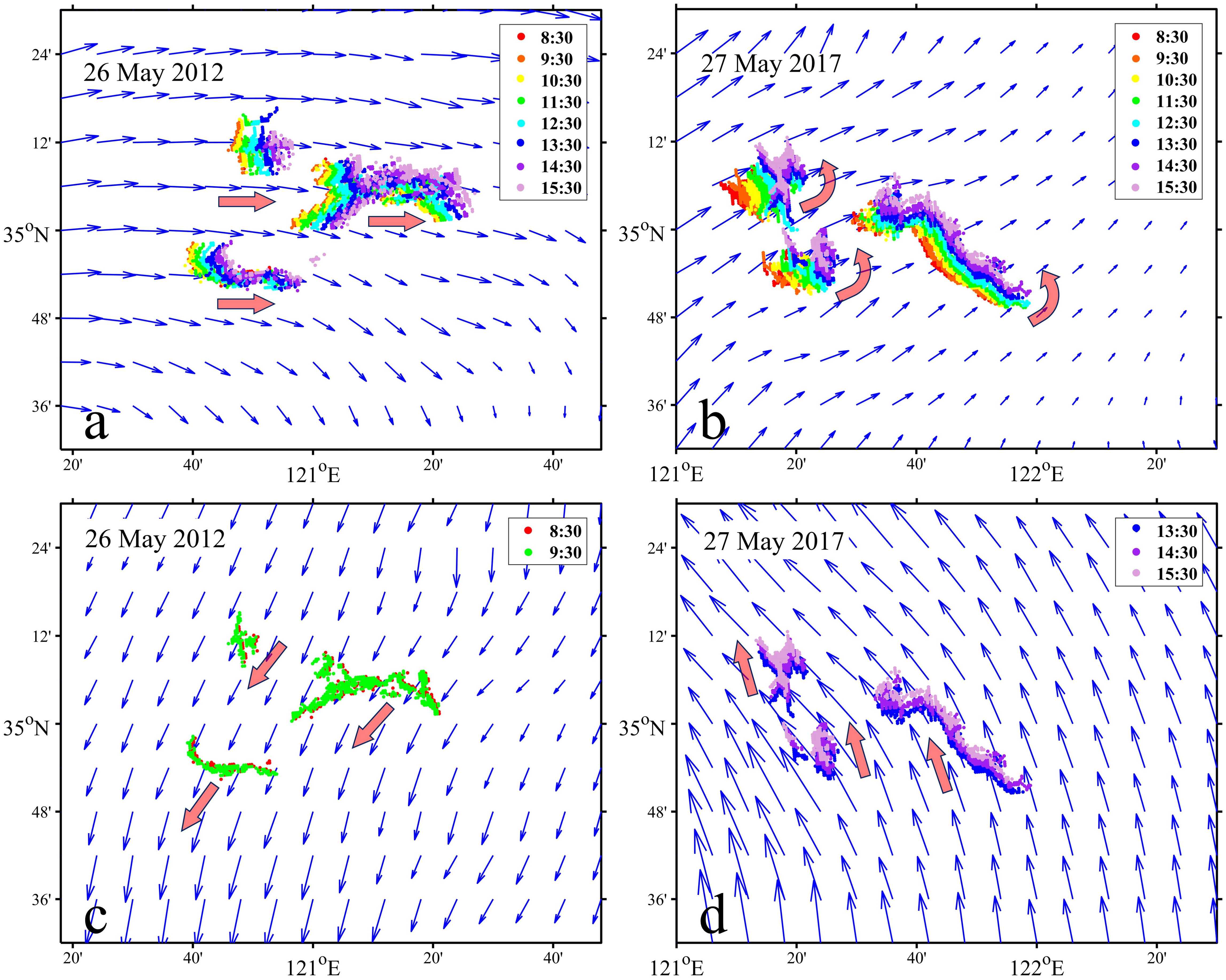
Figure 7 Hourly drifting path of a single Ulva prolifera in a day. The background blue arrow is the corresponding OSU tidal current vector, and the red arrow is the drifting direction of Ulva prolifera. (A) Shows the drifting path of Ulva prolifera extracted on 26 May 2012; (B) Shows the drifting path of Ulva prolifera extracted on 27 May 2017; (C) Shows the drifting path from 8:30 to 9:30 on 26 May; (D) Shows the drifting path from 13:30 to 15:30 on 27 May.

Through the overall observation of the extraction results of single Ulva prolifera algae patch in continuous images, we found that the overall shape of Ulva prolifera patches does not change much during movement in a short time. Therefore, we used the discrimination of similar Ulva prolifera patches in the first and last images (8:30 and 15:30, corresponding to Figures 7A, B) and adjacent time images (corresponding to Figures 7C, D) to measure and calculate the drifting direction of Ulva prolifera and compared the results with the corresponding tidal current data to quantitatively analyze the correlation between the two. Figures 8A, B are sketch maps of the drifting direction of Ulva prolifera in the selected two-day case. The solid and dashed lines of the same color in the graph represent the beginning and end positions of similar Ulva prolifera patches within a day. Figure 8C shows the comparison between the drifting direction of Ulva prolifera and the corresponding tidal current direction. The direction angles of both are distributed between -180° and 180°, which can be confirmed in the tidal current vector of the background field in Figure 7. The coefficient of determination of both is 0.94, which quantitatively proves that the drifting direction of Ulva prolifera is basically consistent with the local tidal current direction within 7 hours of GOCI imaging, and the tidal current is the main factor driving the drift of Ulva prolifera.

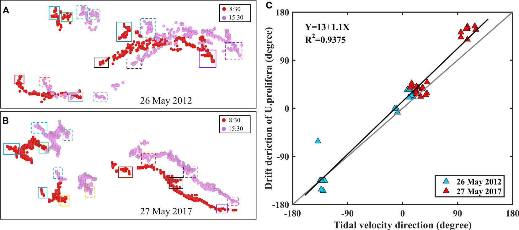
Figure 8 (A, B) Represent sketch maps for measuring the drifting direction of Ulva prolifera. The solid and dotted lines with the same color represent the beginning and end positions of similar Ulva prolifera patches within a day. (C) Shows the comparison diagram between the drifting direction of Ulva prolifera and the corresponding tidal current direction. The gray line is the 1:1 line, and the black line is a straight line of scatter fitting. To ensure the continuity of the direction angle, its range is set to (-180°,180°).

3.2.2 Diurnal variation characteristics of the coverage area

The GOCI can be used to monitor and extract the diurnal variation in the coverage area of Ulva prolifera in the Yellow Sea, which provides favorable data support for responding to green tides disasters. Based on the two-day case data, the NDVI algorithm based on DBSCAN clustering analysis extracted the coverage area of Ulva prolifera for analysis, as shown in Figure 9; the relative change rate of the other seven times was calculated based on the maximum coverage area of the day, as shown in Table 2. In the selected two-day case, the three patches A, B, and C and the total coverage pixels and coverage area of Ulva prolifera all showed a trend of increasing first and then decreasing. On 26 May 2012, the maximum coverage area appeared at 12:30 noon, and the minimum coverage area was at 15:30. The time of the maximum coverage area on 27 May 2017 was 13:30, and the minimum coverage area was at 8:30. At the same time, the change rate of both is the largest when the coverage area is the smallest, which is 0.50 and 0.48, respectively; that is, the area at the time of the monitored maximum coverage area is almost twice that of the minimum coverage area. Within 7 hours of GOCI imaging, the growth and death of Ulva prolifera specimens are unlikely to explain this phenomenon. Therefore, according to previous research results, it is speculated that Ulva prolifera may have undergone vertical migration during this period. The strongest solar radiation at noon is conducive to the photosynthesis of the algae, and the oxygen released forms bubbles to increase the buoyancy of the algae and make it float on the sea surface (Liang et al., 2008).

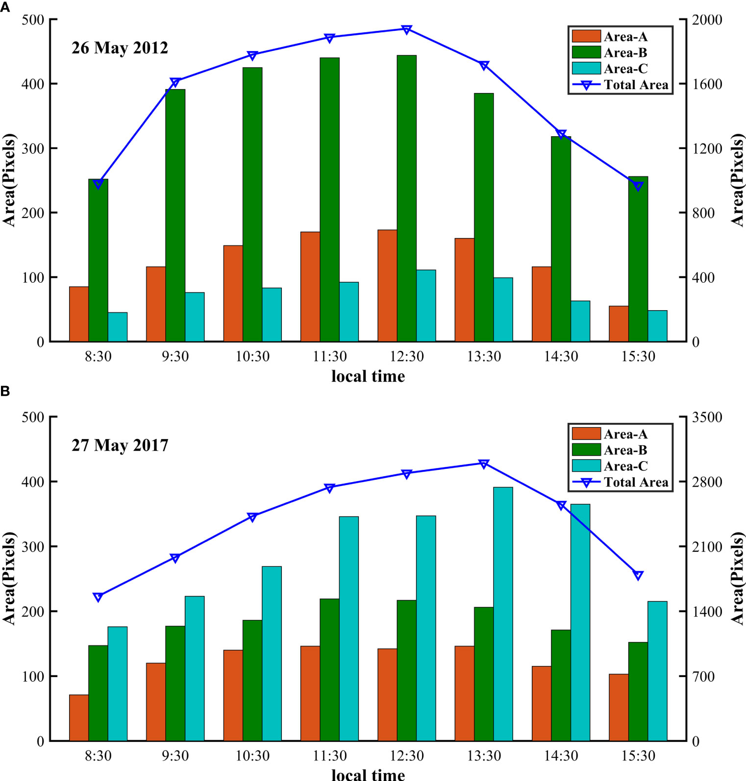
Figure 9 Variation in the coverage area of Ulva prolifera with time. (A) Shows the variation on 26 May 2012, and (B) shows the variation on 27 May 2017, for which the area statistics unit is pixels and 1 pixel represents 0.25 km².

Table 2 Statistics of coverage area characteristics of Ulva prolifera.

4 Discussion

4.1 Influence of tide on the diurnal variation in area

The horizontal tidal current mentioned above is the main factor driving the drift of Ulva prolifera in a day. We suppose that the tidal height variation may also cause the vertical migration of Ulva prolifera, which will lead to diurnal variation in the coverage area. Lou and Hu (2014) mentioned that the short-term changes in the area of harmful algal blooms along the Zhejiang coast may be the result of horizontal dilution caused by tides, possibly due to stronger dilution or mixing of tides in offshore waters. The study area of this paper is in the relatively open sea area northwest of the South Yellow Sea (shown in the red box in Figure 1). The existing tidal stations cannot obtain accurate information on variations in tidal height in the study area, while the OSU tidal current model can obtain tidal height information at any time and location. Therefore, we use the OSU tidal current model to obtain the central tidal height information of the corresponding cases in the study area. Figures 10A, B show the tidal height information obtained by the OSU tidal current model and the tidal height information measured by the tidal station on the corresponding date, where A and B in Figure 1 correspond to Qianliyan and Chengshanjiao, respectively. The tidal height information obtained by the OSU model in one day is basically consistent with the measured tidal height data in terms of change trend and tidal height magnitude, so the OSU tidal height data can also well reflect the variations in tidal height in the study area. Figures 10C, D show the tidal height variation in the two-day case data in the study area. During the GOCI imaging periods, 26 May 2012 was in the ebb tide period, and 27 May 2017 was in the flood tide period. The diurnal variation in the Ulva prolifera coverage area detected within two days tended to increase and then decrease. Therefore, for the non-intertidal open sea, the tidal height change is not the main reason for the diurnal variation in the Ulva prolifera area.

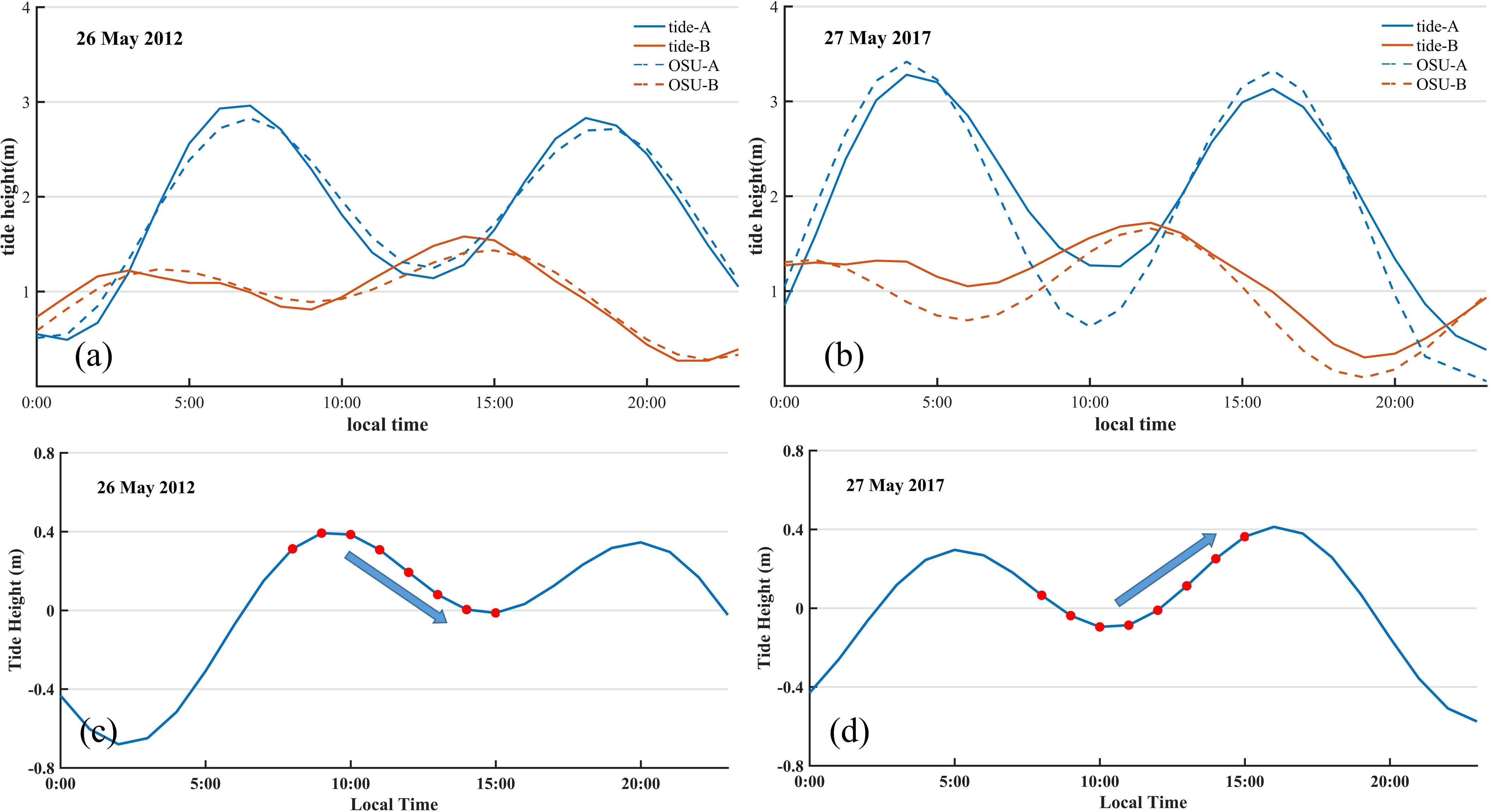
Figure 10 (A, B) Show the tide height information obtained by the OSU tidal current mode and corresponding tidal station. (C, D) Show the tide heights in the study area on 26 May 2012 and 27 May 2017. The dots denote the hourly imaging time of GOCI.

4.2 Influence of NDVI threshold on Ulva prolifera extraction

In the process of extracting Ulva prolifera information, after calculating the NDVI value of the image, it is still necessary to set a threshold to distinguish Ulva prolifera from seawater. In this study, the segmentation threshold is mainly determined by visual interpretation, but there are still mixed pixels of Ulva prolifera and seawater that cannot be fully considered when setting the threshold, resulting in errors in extraction. Therefore, we wanted to investigate the effect of the threshold on the extraction area of Ulva prolifera. In contrast to previous research reports, we used the high temporal resolution characteristics of GOCI data, used the time of the day when the extraction area was the largest as a reference, and changed the NDVI threshold of other times to make the extraction area of 8 moments basically the same to observe the change in the NDVI threshold. Figure 11 shows the change trend of the NDVI threshold when the extraction areas of Ulva prolifera patches A, B and C were consistent at each time of the day on 26 May 2012 and 27 May 2017. The case results of two days show that the NDVI threshold first increases and then decreases. The coverage area in Figure 9 in Section 3.2.2 shows a trend of first increasing and then decreasing, but the NDVI threshold at each time within a day remains unchanged. It can be concluded that in the GOCI imaging time, the extraction area of Ulva prolifera is negatively correlated with the change in the NDVI threshold; that is, for the same image at the same time, the smaller the NDVI threshold is, the larger the extraction area of Ulva prolifera.

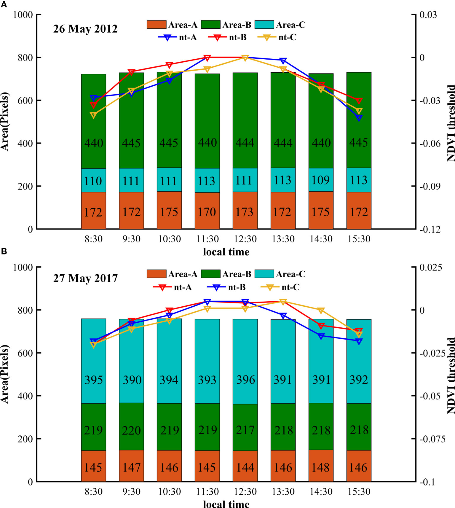
Figure 11 The single Ulva prolifera patch extraction area, which remained consistent, and the daily variation trend of the NDVI threshold. (A) Shows the change trend of three Ulva prolifera patches A, B, and C on 26 May 2012, and (B) shows the change trend of three Ulva prolifera patches A, B, and C on 27 May 2017. nt is the NDVI threshold.

4.3 Causes of diurnal variation in the coverage area

The high temporal resolution of GOCI provides data support for the hourly monitoring of Ulva prolifera in the Yellow Sea. Similar to previous studies, we also concluded that the daily variation in the coverage area of Ulva prolifera tended to increase and then decrease in one day. The reason may be that the buoyancy of Ulva prolifera changed, resulting in vertical migration. In recent years, researchers have explored the biological mechanism of Ulva prolifera given the complex mechanism of green tides (Wang et al., 2020). The results showed that the light compensation point of Ulva prolifera was lower than that of other algae. Usually, the light intensity during the day was much higher than the light compensation point. The lower light compensation points enabled Ulva prolifera to carry out strong photosynthesis and accumulate nutrients when the light intensity was weak (Wang et al., 2010). The mechanism of non-photochemical quenching (NPQ) in Ulva prolifera under high-light conditions is unique, which is significantly different from that in other photosynthetic organisms and can help Ulva prolifera adapt to high-light stress (Gao et al., 2020). In addition, floating Ulva prolifera algae have a unique suspended branching structure, which divides the floating algae into two parts: floating on the sea surface and underwater suspension. If the algae on the sea surface die due to high light stress, the underwater suspension algae can also avoid the high light stress and continue to grow, which also provides a physiological basis for the outbreak of Ulva prolifera and long-distance floating (Wu et al., 2016). Therefore, we speculate that during the seven hours of GOCI imaging, whether it is twilight periods or noon periods, Ulva prolifera can continue photosynthesis, and the continuous generation of bubbles in the algal air sac will not cause significant changes in buoyancy. Vertical migration caused by buoyancy change may not be the main reason for the diurnal variation in the coverage area.

The accuracy of GOCI products is affected not only by the weak light at twilight but also by the difference in satellite-earth imaging paths at different times, which also affects the acquisition of remote sensing information. Figure 12 shows the imaging diagram of the detection area at different times. For the same detection area, the zenith angle of the sun is higher at twilight (8:30 and 15:30) than at noon (12:30), and the solar radiation is lower. In addition, the path from the top of the atmosphere to the detection area at twilight is longer than that at noon (L1 and L3 are both longer than L2), solar radiation is more affected by the atmosphere, and the signal received by the GOCI sensor is weaker. Using the mature Hydrolight-Second Simulation of a Satellite Signal in the Solar Spectrum (6SV) coupled radiation transfer model, Qiao et al. (2021) simulated and calculated the apparent reflectance of the Yellow Sea received by the satellite on 3 May 2019 and compared it with the reflectance obtained by the GOCI sensor. The results showed that the mean absolute percentage error (MAPE) of the bands at 660 nm, 680 nm, 745 nm and 865 nm at twilight was significantly greater than that at noon, and the error first decreased and then increased during the day. The above reasons cause the imaging difference between the GOCI sensor at twilight and noon. Therefore, considering that the number of combined bands used in the NDVI algorithm in this study is 660 nm and 745 nm, combined with the change in the zenith angle of the sun during the GOCI imaging time, we speculated that the change in the intensity of the signal received by the GOCI sensor is the main cause of the diurnal variation in the Ulva prolifera area. That is, within 7 hours of GOCI imaging, there may be no substantial change in the Ulva prolifera coverage area. The signal enhancement received by the GOCI sensor at noon makes the extracted area of Ulva prolifera show a diurnal variation tendency to increase and then decrease.

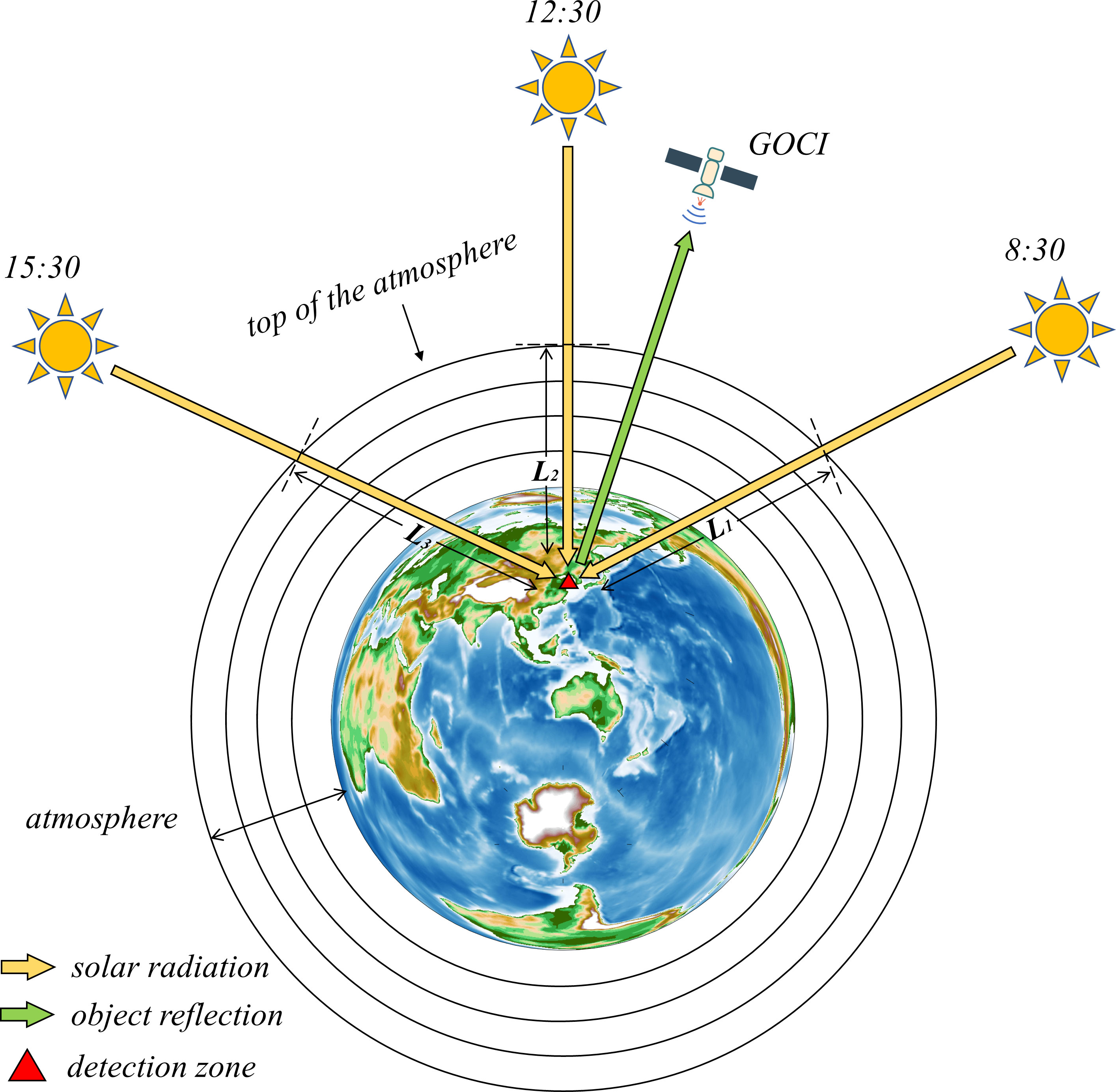
Figure 12 Schematic image of the detection area at different times. Among them, the red triangle represents the location of the detection area, the yellow arrow represents the solar radiation, the green arrow represents the ground object reflection, and L₁, L₂, and L₃ represent the path length of the atmospheric top reaching the detection area at 8:30, 12:30 and 15:30, respectively.

It is still difficult to use traditional algorithms for the AC of GOCI data at high solar zenith angles (> 70°, corresponding to twilight periods). This reduces the amount of data retrieved (Li et al., 2020). The GOCI Rayleigh corrected reflectance product after standard AC processing is affected by the large solar zenith angle and the curvature of the earth during the twilight periods, and there are still some errors (Gordon et al., 1988; Wang, 2002; He et al., 2018). Deviations in data for bands 5 to 8 of the GOCI image are more pronounced during twilight than at noon (Lamquin et al., 2012; Moon et al., 2012; Qiao et al., 2021). The combination of the 5th and 7th bands in the NDVI algorithm was used as the Ulva prolifera detection algorithm in this study. Therefore, the product error caused by the standard AC in the twilight periods will further affect the extraction results of NDVI, and ultimately affect the results of DBSCAN classification in the twilight periods. In this study, a further more accurate AC was achieved by changing the NDVI threshold, which filled the missing data at twilight periods. Figures 13A, B show the distribution of Ulva prolifera patch B 8 times in a day on 26 May 2012, where Figure 13A is the same NDVI threshold at each time, corresponding to Figure 9A. Figure 13B shows the maximum area time as a reference, changing the threshold size so that the area at each time is consistent, corresponding to Figure 11A. Figures 13C, D show the distribution of Ulva prolifera patch A on 27 May 2017. From Figures 13A, C, it can be seen that from 8:30-15:30, the morphology of the independent Ulva prolifera patches has basically not changed, and the location changes are affected by the local tidal current; in Figure 13C, from the beginning to the end of patch A, Ulva prolifera presented a trend of stretching to the north and south ends, which was also affected by the eastward tidal current. The blue portions in Figures 13B, D, which are increments relative to the maximum coverage area after changing the threshold, are essentially distributed at the edges of the original algae and the junction of the blocks. Combined with the extraction results of NDVI in Figure 4, the high value of NDVI is concentrated in the central part of the Ulva prolifera patch, and the blue part corresponds to the easily confused mixed pixels of seawater and Ulva prolifera, which is also the area where the GOCI sensor receives weaker signals during the twilight periods. The distribution of Ulva prolifera extracted at 8:30 and 15:30 in Figure 13A does not easily maintain the current morphology, so the corresponding blue part in Figure 13B should exist, which further supports our speculation.

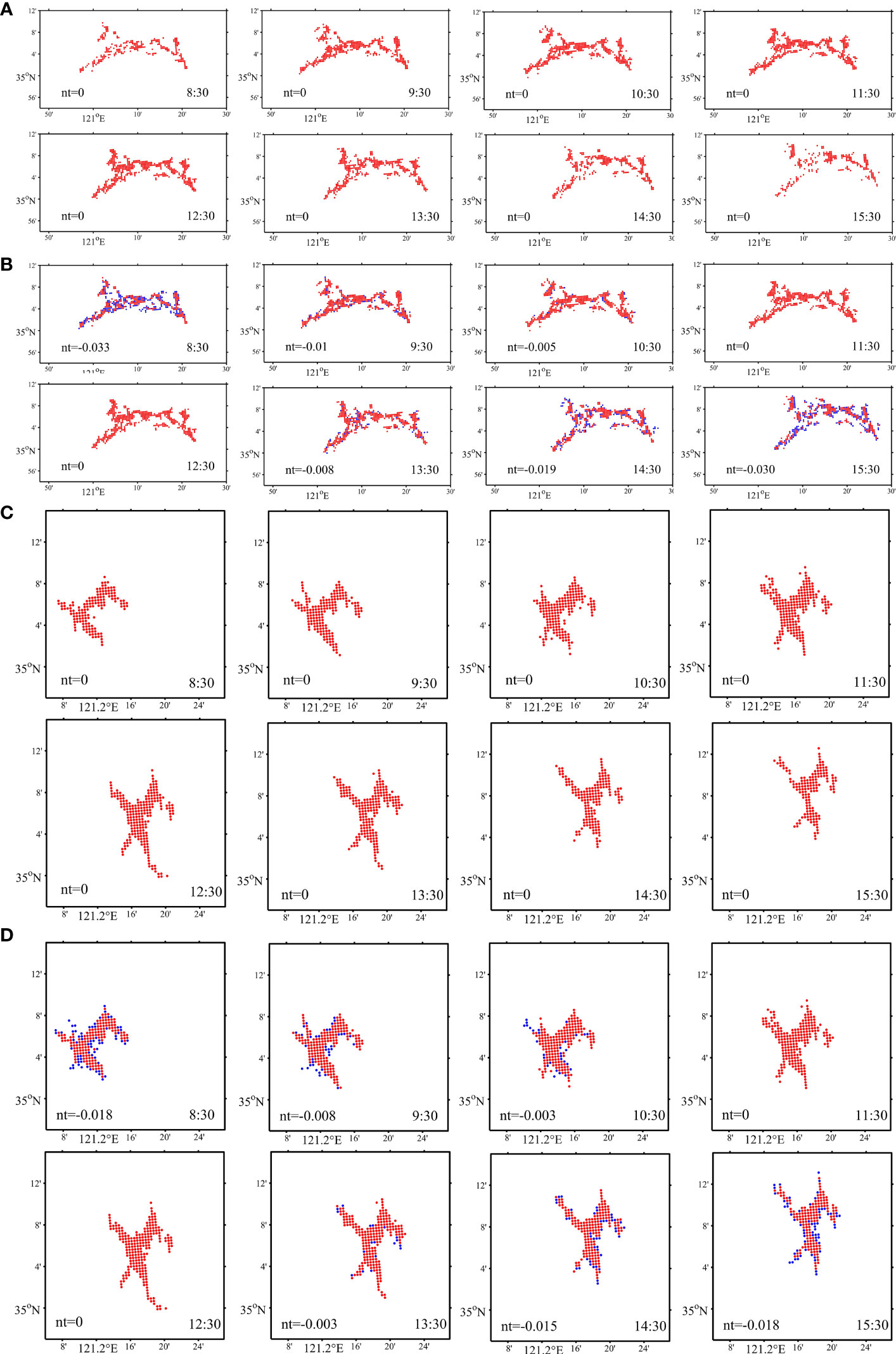
Figure 13 Distribution of Ulva prolifera patch B and patch A on 26 May 2012 and 27 May 2017, respectively. (A, C) show the area distributions with the same threshold at each time, (B, D) are based on the maximum area as a reference, changing the threshold to keep the area consistent at each time, and the blue part is the increased part relative to (A, C), respectively. nt is the NDVI threshold.

5 Conclusions

In this study, considering the high temporal resolution of the GOCI sensor and the patchy distribution of floating Ulva prolifera on the sea surface, we proposed a method of Ulva prolifera extraction based on DBSCAN clustering analysis to quantitatively analyze the diurnal variation characteristics of a single Ulva prolifera patch during GOCI imaging time. This approach was used to extract information from a single Ulva prolifera patch in the Yellow Sea in the same period of 2012 and 2017. The analyzed results showed that during the time of GOCI imaging, the tidal current was the main factor driving the drift of Ulva prolifera, and its direction was consistent with the drifting direction of Ulva prolifera, with a coefficient of determination of 0.94. The detected coverage area of Ulva prolifera tended to increase and then decrease, and the area change rate at twilight compared with that at noon was 0.50.

Using the OSU tidal current model, we can obtained accurate information on tide height changes in the study area. The vertical tide height change was not the main reason for the diurnal variation in Ulva prolifera coverage in the open sea. By keeping the area of Ulva prolifera patches consistent at each time point and observing the change trend of the NDVI threshold, it was concluded that the extraction area of Ulva prolifera has a good negative correlation with the NDVI threshold magnitude.

The lower light compensation points and unique suspended branch structure of Ulva prolifera allow it to float for a long distance, and the water color detection ability of the GOCI sensor also decreased significantly during the twilight periods. For the single Ulva prolifera patch extracted by the proposed method, considering further more accurate AC results, the NDVI threshold was changed to make the coverage area consistent with the maximum coverage area at each time point and compared with the actual extraction results. The results showed that during the twilight periods, compared with the maximum coverage area, the newly added algae were distributed at the edge and block junction of the original algae, which belonged to the confusion area of seawater and Ulva prolifera and was also the area where the GOCI sensor received a weaker signal during the twilight periods. Therefore, we speculated that the change in the intensity of the signal received by the GOCI sensor in one day may be the main reason for the significant diurnal variation in the Ulva prolifera area, rather than the short-term vertical migration of algae. The coverage area of Ulva prolifera may not change substantially. The enhanced signal received by the GOCI sensor at noon indicated that the extracted area of Ulva prolifera had a diurnal variation tendency to increase and then decrease. This also demonstrated the advantage of fine analysis of a single Ulva prolifera patch. However, some field measurements are still needed to verify satellite-based observations.

Data availability statement

The original contributions presented in the study are included in the article/Supplementary Material. Further inquiries can be directed to the corresponding author.

Author contributions

HC: Conceptualization, Methodology, Formal analysis, Writing – original draft, Writing – review & editing. JC: Conceptualization, Methodology, Data curation, Writing – review & editing, Supervision, Funding acquisition. XJ: Data curation. FY: Data curation. FQ: Methodology, Formal analysis. All authors contributed to the article and submitted and approved the submitted section.

Funding

This work was supported by the Funded Program of State Key Laboratory of Satellite Ocean Environment Dynamics (Grant SOEDZZ2203), National Key Research and Development Program of China (Grant 2016YFC1400903), National Natural Science Foundation of China (Grants 42076216,41376184 and 40976109), and NSFC‐Zhejiang Joint Fund for the Integration of Industrialization and Informatization (Grant U1609202).

Acknowledgments

We would like to thank the Korea Ocean Satellite Center (KOSC) for providing GOCI-L1B data and GOCI data processing software (GDPS), the Oregon State University (OSU) for providing TPXO tidal models, the Earth & Space Research (ESR) for providing MATLAB software, and the Tide Model Driver (TMD) package. We also acknowledge tide data support from the National Marine Data Center (NMDC), National Science & Technology Resource Sharing Service Platform of China.

Conflict of interest

The authors declare that the research was conducted in the absence of any commercial or financial relationships that could be construed as a potential conflict of interest.

Publisher’s note

All claims expressed in this article are solely those of the authors and do not necessarily represent those of their affiliated organizations, or those of the publisher, the editors and the reviewers. Any product that may be evaluated in this article, or claim that may be made by its manufacturer, is not guaranteed or endorsed by the publisher.

Supplementary material

The Supplementary Material for this article can be found online at: https://www.frontiersin.org/articles/10.3389/fmars.2023.1177997/full#supplementary-material

References

Ahn J. H., Park Y. J., Ryu J. H., Lee B., Oh I. S. (2012). Development of atmospheric correction algorithm for Geostationary Ocean Color Imager (goci). Ocean ence J. 47 (3), 247–259. doi: 10.1007/s12601-012-0026-2
Amin R., Lewis M. D., Lawson A., Gould R. W. Jr., Martinolich P., Li R. R., et al. (2015). Comparative analysis of GOCI ocean color products. Sensors 15 (10), 25703–25715. doi: 10.3390/s151025703
Cai X., Cui T., Zheng R., Qin P., Mou B. (2014). Comparison of algorithms for green macro-algae bloom detection based on Geostationary Ocean Color Imager. Remote Sens. Inf. 5), 44–50. doi: 10.3969/j.issn.1000-3177.2014.05.008
Çelik M., Dadaşer-Çelik F., Dokuz A. S. (2011). “Anomaly detection in temperature data using DBSCAN algorithm,” in 2011 International Symposium on Innovations in Intelligent Systems and Applications, Istanbul, Turkey. 91–95 (IEEE). doi: 10.1109/inista.2011.5946052
Chen Y., Sun S. D., Zhang H., Wang S. Q., Qiu Z., He Y. (2020). Remote-sensing monitoring of green tide and its drifting trajectories in Yellow Sea based on observation data of Geostationary Ocean Color Imager. Acta Opt. Sin. 40, 301001. doi: 10.3788/AOS202040.0301001
Concha J., Mannino A., Franz B., Kim W. (2019). Uncertainties in the Geostationary Ocean Color Imager (goci) remote sensing reflectance for assessing diurnal variability of biogeochemical processes. Remote Sens. 11 (3), 295;. doi: 10.3390/rs11030295
Cui H., Chen J., Cao Z., Huang H., Gong F. (2022). A novel multi-candidate multi-correlation coefficient algorithm for GOCI-derived sea-surface current vector with OSU tidal model. Remote Sens. 14 (18), 4625. doi: 10.3390/rs14184625
Egbert G. D., Bennett A. F., Foreman M. G. (1994). TOPEX/POSEIDON tides estimated using a global inverse model. J. Geophysical Research: Oceans 99 (C12), 24821–24852. doi: 10.1029/94JC01894
Egbert G. D., Erofeeva S. Y. (2002). Efficient inverse modeling of barotropic ocean tides. J. Atmospheric Oceanic Technol. 19 (2), 183–204. doi: 10.1175/1520-0426(2002)019<0183:EIMOBO>2.0.CO;2
Ester M., Kriegel H. P., Sander J., Xu X. (1996). A density-based algorithm for discovering clusters in large spatial databases with noise. In Proceedings of the Second International Conference on Knowledge Discovery and Data Mining (KDD’96) 96, 226–231.
Gao S., Zheng Z., Wang J., Wang G. (2020). Slow zeaxanthin accumulation and the enhancement of CP 26 collectively contribute to an atypical non-photochemical quenching in macroalga Ulva prolifera under high light. J. phycology 56 (2), 393–403. doi: 10.1111/jpy.12958
Gordon H. R., Brown J. W., Evans R. H. (1988). Exact rayleigh scattering calculations for use with the nimbus-7 coastal zone color scanner. Appl. Optics 27 (5), 862–871. doi: 10.1364/AO.27.000862
Hartigan J. A., Wong M. A. (1979). Algorithm AS 136: A k-means clustering algorithm. J. R. Stat. society. Ser. c (applied statistics) 28 (1), 100–108. doi: 10.2307/2346830
He X., Stamnes K., Bai Y., Li W., Wang D. (2018). Effects of earth curvature on atmospheric correction for ocean color remote sensing. Remote Sens. Environ. 209, 118–133. doi: 10.1016/j.rse.2018.02.042
Hsueh Y. (1988). Recent current observations in the eastern Yellow Sea. J. Geophysical Research: Oceans 93 (C6), 6875–6884. doi: 10.1029/jc093ic06p06875
Hu C. (2009). A novel ocean color index to detect floating algae in the global oceans. Remote Sens. Environ. 113 (10), 2118–2129. doi: 10.1016/j.rse.2009.05.012
Hu C., He M. X. (2008). Origin and offshore extent of floating algae in Olympic sailing area. Eos Trans. Am. Geophysical Union 89 (33), 302–303. doi: 10.1029/2008EO330002
Hu C., Li D., Chen C., Ge J., Muller-Karger F. E., Liu J., et al. (2010). On the recurrent Ulva prolifera blooms in the Yellow Sea and East China Sea. J. Geophysical Research: Oceans 115 (C5). doi: 10.1029/2009JC005561
Hu Z., Wang D. P., Pan D., He X., Miyazawa Y., Bai Y., et al. (2016). Mapping surface tidal currents and Changjiang plume in the East China Sea from Geostationary Ocean Color Imager. J. Geophysical Research: Oceans 121 (3), 1563–1572. doi: 10.1002/2015JC011469
Hu X., Wu X., Meng X., Schabenberger O., SAS Institute Inc (2014) Methods and systems for data reduction in cluster analysis in distributed data environments. Available at: https://patents.google.com/patent/US20140330826A1/en.
Ji G., Zhao B. (2015). Research progress on spatiotemporal trajectory big data pattern mining. J. Data Acquisition Process. 30, 47–58. doi: 10.16337/j.1004-9037.2015.01.004
Jiang L., Wang M. (2016). Diurnal currents in the Bohai Sea derived from the Korean Geostationary Ocean Color Imager. IEEE Trans. Geosci. Remote Sens. 55 (3), 1437–1450. doi: 10.1109/tgrs.2016.2624220
Jiang Y., Zhang Q. (2017). Hurricane trajectory clustering algorithm based on grey method and structural distance. Syst. Engineering-Theory Pract. 37 (4), 1046–1055. doi: 10.12011/1000-6788(2017)04-1046-10
Ju-Long D. (1982). Control problems of grey systems. Syst. Control Lett. 1 (5), 288–294. doi: 10.1016/S0167-6911(82)80025-X
Lamquin N., Mazeran C., Doxaran D., Ryu J. H., Park Y. J. (2012). Assessment of GOCI radiometric products using MERIS, MODIS and field measurements. Ocean Sci. J. 47 (3), 287–311. doi: 10.1007/s12601-012-0029-z
Li H., He X., Bai Y., Shanmugam P., Park Y. J., Liu J., et al. (2020). Atmospheric correction of geostationary satellite ocean color data under high solar zenith angles in open oceans. Remote Sens. Environ. 249, 112022. doi: 10.1016/j.rse.2020.112022
Li H., He X., Shanmugam P., Bai Y., Wang D., Huang H., et al. (2019). Radiometric sensitivity and signal detectability of ocean color satellite sensor under high solar zenith angles. IEEE Trans. Geosci. Remote Sens. 57 (11), 8492–8505. doi: 10.1109/TGRS.2019.2921341
Li H., He X., Tao B., Wang D. (2018). Research on chlorophyll detection ability under high solar zenith angle. Haiyang Xuebao 40 (11), 128–140. doi: 10.3969/j.issn.0253-4193.2018.11.013
Li J., Liang Y., Zhang J., Yang J., Song P., Cui W. (2019). A new automatic oceanic mesoscale eddy detection method using satellite altimeter data based on density clustering. Acta Oceanologica Sin. 38 (5), 134–141. doi: 10.1007/s13131-019-1447-x
Liang Z., Lin X., Ma M., Zhang J., Yan X., Liu T. (2008). A preliminary study of the Enteromorpha prolifera drift gathering causing the green tide phenomenon. Period Ocean Univ China 38, 601–604. doi: 10.3969/j.issn.1672-5174.2008.04.031
Lie H. J., Lee S., Cho C. H. (2002). Computation methods of major tidal currents from satellite-tracked drifter positions, with application to the Yellow and East China Seas. J. Geophysical Research: Oceans 107 (C1), 3–1. doi: 10.1029/2001JC000898
Liu D., Keesing J. K., He P., Wang Z., Shi Y., Wang Y. (2013). The world's largest macroalgal bloom in the Yellow Sea, China: formation and implications. Estuarine Coast. Shelf Sci. 129, 2–10. doi: 10.1016/j.ecss.2013.05.021
Lou X., Hu C. (2014). Diurnal changes of a harmful algal bloom in the East China Sea: Observations from GOCI. Remote Sens. Environ. 140, 562–572. doi: 10.1016/j.rse.2013.09.031
Manavalan R., Thangavel K. (2011). “TRUS image segmentation using morphological operators and DBSCAN clustering,” in 2011 World Congress on information and communication technologies, Mumbai, India. 898–903 (IEEE). doi: 10.1109/wict.2011.6141367
Matthew M. W., Adler-Golden S. M., Berk A., Felde G., Shippert M. (2003). Atmospheric correction of spectral imagery: evaluation of the FLAASH algorithm with AVIRIS data. In Proceedings of the 31st Applied Image Pattern Recognition Workshop on From Color to Hyperspectral: Advancements in Spectral Imagery Exploitation (AIPR ’02). IEEE Computer Society, USA, 157–163. doi: 10.1117/12.499604
Moon J. E., Park Y. J., Ryu J. H., Choi J. K., Ahn J. H., Min J. E., et al. (2012). Initial validation of GOCI water products against in situ data collected around Korean peninsula for 2010–2011. Ocean Sci. J. 47 (3), 261–277. doi: 10.1007/s12601-012-0027-1
Otsu N. (1979). A threshold selection method from gray-level histograms. IEEE Trans. systems man cybernetics 9 (1), 62–66. doi: 10.1109/tsmc.1979.4310076
Padman L., Erofeeva S. (2005). Tide model driver (TMD) manual (Earth and Space research). Available at: https://www.esr.org/polar_tide_models/README_TMD.pdf.
Qi L., Hu C., Wang M., Shang S., Wilson C. (2017). Floating algae blooms in the East China Sea. Geophysical Res. Lett. 44 (22), 11–501. doi: 10.1002/2017GL075525
Qiao F., Chen J., Xu Y. (2021). Usability analysis GOCI twilight periods radiative transfer model data. Mar. Inf. 36 (1), 12. doi: 10.19661/j.cnki.mi.2021.01.005
Qiao F., Dai D., Simpson J., Svendsen H. (2009). Banded structure of drifting macroalgae. Mar. pollut. Bull. 58 (12), 1792–1795. doi: 10.1016/j.marpolbul.2009.08.006
Ryu J. H., Ishizaka J. (2012). GOCI data processing and ocean applications. Ocean Sci. J. 47 (3), 221. doi: 10.1007/s12601-012-0023-5
Sezgin M., Sankur B. (2004). Survey over image thresholding techniques and quantitative performance evaluation. J. Electronic Imaging 13 (1), 146–165. doi: 10.1117/1.1631315
Shanmugam P., Suresh M., Sundarabalan B. (2013). Osabt: an innovative algorithm to detect and characterize ocean surface algal blooms. IEEE J. Selected Topics Appl. Earth Observations Remote Sens. 6 (4), 1879–1892. doi: 10.1109/JSTARS.2012.2227993
Shi H., Ma X. (2018). Two-stage outlier detection method based on DBSCAN clustering and LAOF of hybrid data. J. Chin. Comput. Syst. 39 (001), 74–77. doi: 10.3969/j.issn.1000-1220.2018.01.016
Shi W., Wang M. (2009). Green macroalgae blooms in the Yellow Sea during the spring and summer of 2008. J. Geophysical Research: Oceans 114 (C12). doi: 10.1029/2009JC005513
Smetacek V., Zingone A. (2013). Green and golden seaweed tides on the rise. Nature 504 (7478), 84–88. doi: 10.1038/nature12860
Son Y. B., Choi B. J., Kim Y. H., Park Y. G. (2015). Tracing floating green algae blooms in the Yellow Sea and the East China Sea using GOCI satellite data and Lagrangian transport simulations. Remote Sens. Environ. 156, 21–33. doi: 10.1016/j.rse.2014.09.024
Son Y. B., Min J. E., Ryu J. H. (2012). Detecting massive green algae (Ulva prolifera) blooms in the Yellow Sea and East China Sea using Geostationary Ocean Color Imager (GOCI) data. Ocean Sci. J. 47 (3), 359–375. doi: 10.1007/s12601-012-0034-2
Song D., Gao Z., Xu F., Ai J., Ning J. C., Shang W. T., et al. (2018). Spatial and temporal variability of the green tide in the South Yellow Sea in 2017 deciphered from the GOCI image. Oceanologia Limnology Sinic 49, 1068–1074. doi: 10.11693/hyhz20171200330
Teague W. J., Perkins H. T., Hallock Z. R., Jacobs G. A. (1998). Current and tide observations in the southern Yellow Sea. J. Geophysical Research: Oceans 103 (C12), 27783–27793. doi: 10.1029/98JC02672
Valiela I., McClelland J., Hauxwell J., Behr P. J., Hersh D., Foreman K. (1997). Macroalgal blooms in shallow estuaries: controls and ecophysiological and ecosystem consequences. Limnology oceanography 42 (5part2), 1105–1118. doi: 10.4319/lo.1997.42.5_part_2.1105
Wang M. H. (2002). The rayleigh lookup tables for the seawifs data processing: accounting for the effects of ocean surface roughness. Int. J. Remote Sens. 23 (13), 2693–2702. doi: 10.1080/01431160110115591
Wang M., Gordon H. R. (1994). A simple, moderately accurate, atmospheric correction algorithm for seawifs. Remote Sens. Environ. 50 (3), 231–239. doi: 10.1016/0034-4257(94)90073-6
Wang Y., Huo Y., Cao J., Chen L., He P. (2010). Influence of low temperature and low light intensity on growth of Ulva compessa. J. Fishery Sci. China 17 (3), 593–599. doi: 10.3724/SP.J.1011.2010.01351
Wang Q., Qin. P., Zhao X. (2017). Advances in the application study of the first Geostationary Ocean Color Imager. Coast. Eng. 2), 71–78. doi: 10.3969/j.issn.1002-3682.2017.02.009
Wang G., Wang H., Gao S., Huan L., Wang L., Gu W., et al. (2020). Study on the biological mechanism of green tide. Oceanologia Limnologia Sin. 51 (4), 20. doi: 10.11693/hyhz20200300078
Wishert D. (1969). Mode analysis: a generalization of nearest neighbour which reduces chaining effects (with discussion). Numerical taxonomy, 282–311.
Wu Q., Zhang J., Zhao S., Liu C., Zhang H., Ji X., et al. (2016). An adjustment mechanism to high light intensity for free-floating Ulva in the Yellow Sea. J. Shanghai Ocean Univ. 25 (1), 97–105. doi: 10.12024/jsou.20150301380
Xing Q., Hu C. (2016). Mapping macroalgal blooms in the Yellow Sea and East China Sea using HJ-1 and Landsat data: Application of a virtual baseline reflectance height technique. Remote Sens. Environ. 178, 113–126. doi: 10.1016/j.rse.2016.02.065
Ye N. H., Zhang X. W., Mao Y. Z., Liang C. W., Xu D., Zou J., et al. (2011). ‘Green tides’ are overwhelming the coastline of our blue planet: taking the world’s largest example. Ecol. Res. 26 (3), 477–485. doi: 10.1007/s11284-011-0821-8
Yu R. C., Liu D. Y. (2016). Harmful algal blooms in the coastal waters of China: current situation, long-term changes and prevention strategies. Bull. Chin. Acad. Sci. 31 (10), 1167–1174. doi: CNKI:SUN:KYYX.0.2016-10-006
Keywords: Ulva prolifera, GOCI, remote sensing detection, NDVI, DBSCAN clustering analysis, diurnal variation
Citation: Cui H, Chen J, Jiang X, Fu Y and Qiao F (2023) A novel quantitative analysis for diurnal dynamics of Ulva prolifera patch in the Yellow Sea from Geostationary Ocean Color Imager observation. Front. Mar. Sci. 10:1177997. doi: 10.3389/fmars.2023.1177997
Received: 02 March 2023; Accepted: 11 July 2023;
Published: 28 July 2023.
Edited by:
Atsushi Matsuoka, University of New Hampshire, United StatesReviewed by:
Joji Ishizaka, Nagoya University, JapanShengqiang Wang, Nanjing University of Information Science and Technology, China
Bror Jonsson, Plymouth Marine Laboratory, United Kingdom
Copyright © 2023 Cui, Chen, Jiang, Fu and Qiao. This is an open-access article distributed under the terms of the Creative Commons Attribution License (CC BY). The use, distribution or reproduction in other forums is permitted, provided the original author(s) and the copyright owner(s) are credited and that the original publication in this journal is cited, in accordance with accepted academic practice. No use, distribution or reproduction is permitted which does not comply with these terms.
*Correspondence: Jianyu Chen, chenjianyu@sio.org.cn