Climate drivers of Southern Ocean phytoplankton community composition and potential impacts on higher trophic levels

1 Introduction

The Southern Ocean environment is changing rapidly under the influence of anthropogenic climate warming, with implications for the marine ecosystem (Morley et al., 2020). Southern Ocean primary productivity and phytoplankton community composition, for example, play an important role in regulating global ocean productivity and carbon cycling (Sarmiento et al., 2004; Krumhardt et al., 2020; Nissen et al., 2021)—and influence how carbon and energy are transferred up local food chains. Primary productivity in the Southern Ocean ultimately supports higher trophic level organisms such as fish, seabirds, seals, and whales. Climate-driven changes in primary productivity, as well as shifts in plankton community composition, may yield cascading effects on the broader marine ecosystem (Deppeler and Davidson, 2017). Indeed, shifts in Antarctic phytoplankton communities are already being observed (Mendes et al., 2018; Lima et al., 2019; Henley et al., 2020). In this paper, we examine simulations conducted with an Earth system model (ESM) run under a high emission scenario as a means of investigating possible bottom-up drivers of change in the Southern Ocean marine ecosystem and potential effects on higher trophic levels.

The Southern Ocean is a high nutrient, low chlorophyll (HNLC) region, where iron, light, and low temperatures play important roles in regulating phytoplankton growth. Aside from shelf regions naturally fertilized by iron (e.g., Blain et al., 2007; Morley et al., 2020), iron supply over most of the Southern Ocean is a primary resource limiting phytoplankton growth. Ice cover is also an important influence on primary production, limiting the availability of irradiance under extensive ice cover. Variation of light and iron supply in the Southern Ocean has been observed to drive differences in community composition (Feng et al., 2010; Mendes et al., 2018); changes in these limitation factors, along with warming waters, could induce shifts in phytoplankton community composition (Bopp et al., 2013; Leung et al., 2015; Moore et al., 2018; Boyd, 2019; Ferreira et al., 2020).

The imprint of anthropogenic climate change on the Southern Ocean manifests through warming, a poleward shift in the core of the westerly winds, and reductions in sea ice cover (Leung et al., 2015; Petrou et al., 2016). Changes in the westerly wind field, which result from ozone depletion and CO₂-driven tropospheric warming, have been documented in observational and modeling studies (e.g., Grise et al., 2013; Kajtar et al., 2021). These changes are associated with increasingly positive phases of the Southern Annular Mode (SAM) and may impact cloudiness, with implications for insolation at the ocean surface (Grise et al., 2013; Kelleher and Grise, 2021). Moreover, changes in wind and buoyancy forcing of the surface ocean play an important role in mediating the supply of iron to the euphotic zone (Henley et al., 2020). In addition to shifts in iron supply, projected loss of Antarctic sea ice will lead to increases in light penetration in the sea ice zone.

These changes may exert selection pressure structuring phytoplankton community composition through competition for resources. Cell size, for example, is a dominant trait, with nutrient-limited regimes preferencing smaller organisms, which have more efficient nutrient uptake abilities due to greater surface-area to volume ratios (Chisholm, 1992). Phytoplankton size is a significant determinant of the zooplankton grazer community; thus, the dominant type of phytoplankton influences how energy is passed up the food chain in marine ecosystems (Moline et al., 2004; Eddy et al., 2021). For example, along the Western Antarctic Peninsula (WAP), a shift from diatoms to cryptophytes was observed over the period 1991 to 1996, which may have contributed to a shift from krill to salps as the dominant zooplankton group (Moline et al., 2004). Indeed, krill preferentially consume diatoms over smaller phytoplankton species, such as cryptophytes and Phaeocystis (Haberman et al., 2003; Hellessey et al., 2020; Pauli et al., 2021). These changes have the potential to affect higher trophic levels; for example, Saba et al. (2014) showed that there are more krill present in penguin diets during years when diatoms dominate the WAP phytoplankton assembleges, as opposed to cryptophytes. These observations suggest that climate-related shifts in phytoplankton communities in the Southern Ocean could affect food resources for upper trophic levels of Antarctic ecosystems (e.g., penguins).

Ecosystem transfer efficiency (ETE) quantifies the amount of energy at a top trophic level relative to that at the base of the food web (see also Maureaud et al., 2017; Petrik et al., 2019). In general, short trophic pathways in highly productive systems lead to higher ETE than longer pathways typical of nutrient-limited regimes dominated by small-celled organisms (Hunt et al., 2021). ETE in oligotrophic regimes is low because the small phytoplankton, favored by nutrient limitation, support small zooplankton that are, in turn, consumed by slightly larger organisms, yielding multiple trophic links between primary production and forage fish or mammals. Oligotrophic systems, therefore, yield poor ETE, but are highly efficient at recycling nutrients within the planktonic system, moving energy around the microbial loop rather than passing it up the food chain (Sommer et al., 2002; Armengol et al., 2019). This contrasts with more productive systems in which large phytoplankton predominate. Large phytoplankton, such as diatoms, can be directly consumed by large zooplankton, such as copepods or krill, which, in turn, can be consumed directly by fish or other marine predators (Moline et al., 2004). Systems dominated by large phytoplankton, therefore, tend to be characterized by fewer zooplankton steps linking primary producers to higher trophic levels and thus tend to have higher ETE. Changes in climate have the potential to drive shifts in ETE through bottom-up forcing affecting phytoplankton assemblages. It is an open question, however, how these effects might play out over the coming decades in the Southern Ocean.

Here, we document climate-driven rearrangements of the phytoplankton community composition in the productive Southern Ocean ecosystem from a large ensemble of ESM simulations that were run under a high emission scenario. While our model does not explicitly simulate higher-trophic level dynamics, we reference scaling relationships to project the likely impact of the changes on large zooplankton and food resources available for higher-trophic level consumption. The changes in climate variables projected by the model are highly uncertain and our objectives are not to propose these results as a definitive future scenario. Rather, our primary objective is to demonstrate mechanistic connections between climate and phytoplankton that might drive important bottom-up variations in the ecosystem as a whole.

2 Material and methods

2.1 CESM large ensemble

We used the Community Earth System Model (version 1) Large Ensemble (CESM1-LE) (Kay et al., 2015) to analyze changes in Southern Ocean phytoplankton community composition. Briefly, CESM version 1 (CESM1) was run “fully coupled,” with ocean, land, sea ice, and biogeochemistry at the nominal 1° resolution. Ensemble member 1 was initialized at a randomly chosen year of the preindustrial control (year 402) and integrated from 1850 to 2100, forced by historical (1850–2005) and then Representative Concentration Pathway 8.5 (RCP8.5; 2006–2100) atmospheric CO₂ concentrations and other radiative forcing. The other ensemble members (for a total of 34 ensemble members) of the CESM1-LE were initialized from the 1920 state of ensemble member 1 with round-off level differences in the air temperature field (i.e., O(10^-14) K) and run under historical and then RCP8.5 forcing (the same forcing as ensemble member 1); these small differences rapidly accumulate to yield divergent solutions and ensemble spread that is representative of the intrinsic variability of the Earth system (Deser et al., 2020). The ocean biogeochemistry simulated by the CESM1-LE has been examined in several publications (e.g., Long et al., 2016; Lovenduski et al., 2016; Krumhardt et al., 2017; Freeman et al., 2018; Sylvester et al., 2021). All the simulations used in this study were therefore run under the same historical and future warming scenario (RCP8.5), but they have different phasing of internal climate variability. Notably, the large ensemble provides a framework to explicitly separate the “externally-forced”, or deterministic, response of the climate system to anthropogenic activity from that associated with natural variability, which arises due to interactions within the climate system (Hasselmann, 1976). Our interest in this analysis is mostly confined to the secular change in climate associated with the forced signal.

2.2 The CESM marine ecosystem

The CESM1 ecosystem model is called the “Biogeochemical Elemental Cycle” (BEC) model; it has three phytoplankton functional types (PFTs): small phytoplankton, diatoms, and diazotrophs (Moore et al., 2002; Long et al., 2013; Moore et al., 2013). Small phytoplankton tend to dominate in warmer, nutrient-limited regimes, whereas diatoms are more prevalent in colder, nutrient-rich oceanic regions. Diazotrophs are able to fix atmospheric nitrogen and comprise a small fraction of total globally integrated net primary production by phytoplankton (Krumhardt et al., 2017). Diazotrophs are not included in the analysis in this study, however, as they are strongly limited by temperature and thus confined to warmer waters (>15^°C).

2.2.1 Phytoplankton growth

The BEC parameterizations describing how phytoplankton interact with environmental drivers are documented in Moore et al. (2002; 2004; 2013). For the purpose of this study, we further elaborate on certain parameterizations that are important for driving the Southern Ocean phytoplankton community hypotheses outlined in this study. Phytoplankton growth rates (μ) are parameterized as the product of the resource-unlimited growth rate (μ_ref) at a reference temperature (30^oC), and a temperature scaling function (T_lim), μ_T=μ_refT_lim, as well as nutrient (N_lim) and irradiance (I_lim) limitation terms:

Small phytoplankton and diatoms have the same maximum growth rate (Table 1). They also have the same temperature limitation function, parameterized as a Q10 (temperature coefficient) curve:

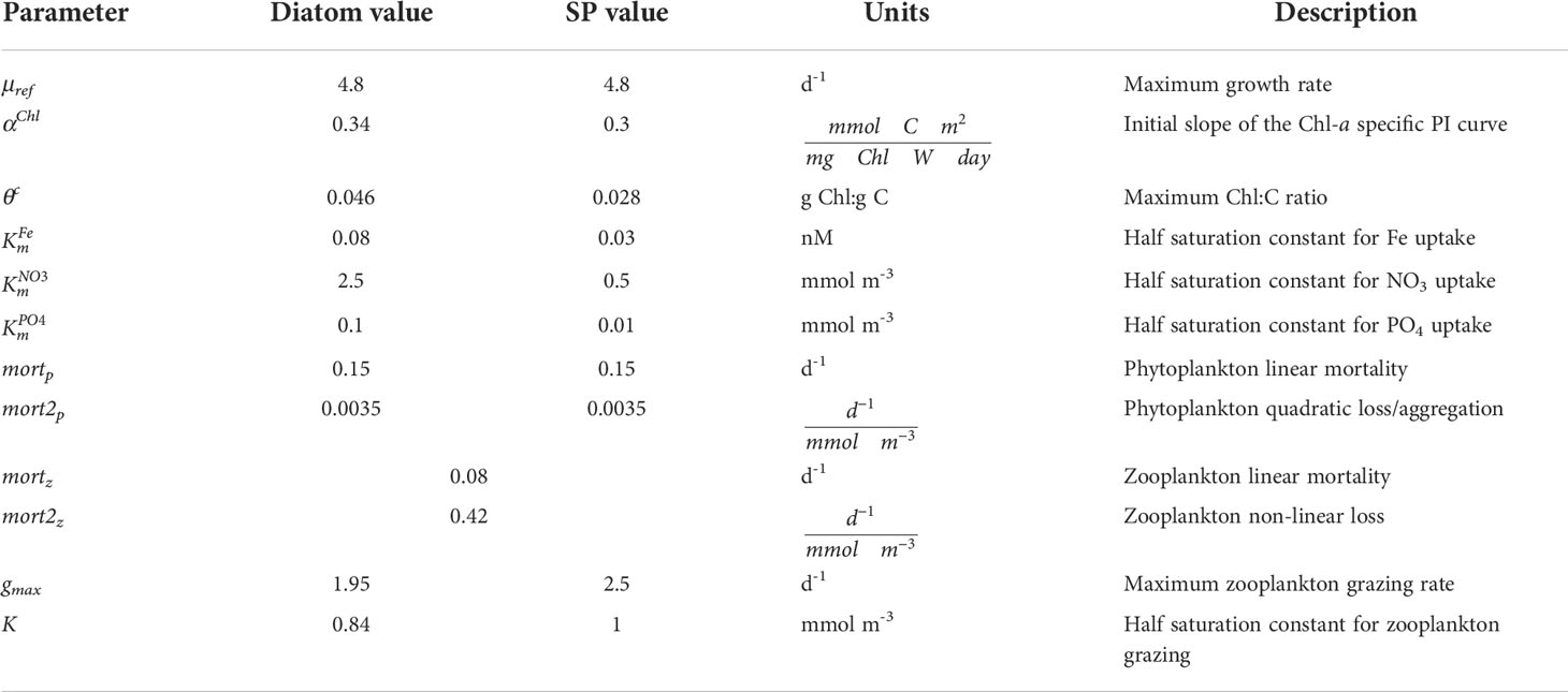
Table 1 Parameter values for diatoms, small phytoplankton (SP), and zooplankton for the CESM1 ocean ecosystem model used in the CESM1-LE.

where Q10=2 in CESM1.

Light limitation (I_lim) of phytoplankton is described by the following equation originally from Geider et al. (1997):

where α^Chl is the initial slope of the chlorophyll-a specific photosynthesis-irradiance (PI) curve and θ^c is the chlorophyll to carbon ratio, I is irradiance as photosynthetically active radiation (PAR; W m^-2), and N_lim is the fractional nutrient limitation term for the most limiting nutrient (see below).

Small phytoplankton have a higher α^Chl than diatoms (Table 1). Diatoms, however, have a higher maximum θ^c which enables greater increases in chlorophyll content through photoadaptation, thereby conferring an advantage in low light conditions (Table 1). We conducted a literature review of maximum θ^c focusing on temperate and polar phytoplankton species; indeed this difference in maximum θ^c between diatoms and other phytoplankton species (e.g., coccolithophores, dinoflagellates, and marine cyanobacteria) is supported by these studies (Figure S1).

Nutrient limitation in CESM is represented via Michaelis-Menten uptake kinetics. Since the Southern Ocean is rich in macronutrients, it is mainly iron (Fe) that limits phytoplankton growth (see Moore et al., 2002):

where Fe is the ambient iron concentration and $K_m^{Fe}$ is the half saturation constant for iron. In general, small phytoplankton have an advantage when nutrients are limiting due to larger surface area to volume ratio, as diffusion limits how fast large phytoplankton like diatoms may grow when nutrients are scarce (Chisholm, 1992). This is parameterized in CESM by the fact that small phytoplankton have smaller nutrient half saturation constants than diatoms (Table 1).

In summary, the small phytoplankton PFT tends to fare better under nutrient limited, high light conditions and diatoms proliferate faster when light is low and nutrients are high. Despite the relatively simplistic PFT groupings in CESM, the underlying parameterizations capture the distinction between “gleaners” (small phytoplankton) and “opportunists” (diatoms); shifts in community composition arising due to changing environmental conditions, therefore, reflect preferential selection for traits defining these respective ecological strategies (Dutkiewicz et al., 2013). Notably, the dominant physiological distinctions between diatoms and small phytoplankton in terms of growth in CESM1 relate to light and nutrient limitation, since (in BEC) the direct effect of temperature affects both diatoms and small phytoplankton growth rates equally (i.e., Eq. 1). However, since μ_T also appears in the non-linear light limitation term (Equation 3), there is a more subtle effect of changes in temperature (e.g., warming) through light limitation and photoadaptation. While warmer conditions lower the I_lim term for both phytoplankton types, the impact on small phytoplankton is stronger, giving diatoms a competitive advantage with respect to light limitation under increasing temperature.

2.2.2 Grazing and other phytoplankton loss

Both diatoms and small phytoplankton in BEC are subject to the same linear mortality rate (mort_p; Table 1), which is scaled by T_lim, the Q10 function described above for phytoplankton growth (Equation 2). T_lim also scales phytoplankton density-dependent quadratic losses (same for both phytoplankton groups; mort2_p in Table 1), which is meant to represent phytoplankton losses from aggregation.

Both phytoplankton groups are grazed by a generic zooplankton functional type. Grazing (G) is computed using a Holling Type III relationship:

where g_max is the maximum grazing rate, T_lim is the same Q10 function as described above for phytoplankton (Equation 2), Z is the zooplankton concentration, P is the phytoplankton concentration, and K is the half-saturation constant for grazing. The parameters in this equation, g_max and K, are different for diatom and small phytoplankton PFTs. The gmax is 2.5 d^-1 for small phytoplankton and 1.95 d^-1 for diatoms, reflecting slower grazing rates for larger zooplankton (Hansen et al., 1997), which, in general, feed on large phytoplankton like diatoms. The value of K is also smaller for diatoms (0.84 mmol m^-3 versus 1 mmol m^-3 for small phytoplankton), which is meant to reflect the fact that larger zooplankton tend to be more apt at catching larger prey. The gross growth efficiency for zooplankton grazing on small phytolankton and diatoms in CESM1 is 0.3 (Straile, 1997), such that 30% of grazed biomass is routed to zooplankton biomass; the rest is routed to dissolved inorganic carbon (DIC), dissolved organic carbon (DOC), and sinking particular organic carbon (POC). Zooplankton loss terms include temperature-dependent (Q10) linear and non-linear, density-dependent mortality terms, where the nonlinear term is meant to represent losses from predation.

The values for mort_z and mort2_z in this equation are 0.08 d^-1 and 0.42 d^-1, respectively (Table 1). The value for the linear mortality, mort_z, represents the natural mortality rate for a generic zooplankton type that has a turnover time (i.e., mean life span) of approximately 12.5 days, while the non-linear term (mort2_z), which represents predation by higher trophic levels, was tuned to achieve reasonable zooplankton biomass distribution.

2.2.3 Model evaluation of phytoplankton distribution and phenology

We evaluated the CESM1-LE simulation of the spatial distribution of phytoplankton biomass by comparing modeled surface chlorophyll (chlorophyll in the top layer of the ocean model, top 10m) with satellite-derived ocean chlorophyll. We used the GlobColour merged chlorophyll product (Garnesson et al., 2019) to compare to the CESM1-LE ensemble mean chlorophyll over the period 1998 to 2005 (1998 is the first year satellite-derived chlorophyll and 2005 is the last year of the historical forcing of the CESM1-LE simulations, after which it is RCP8.5 forcing). Figure S2 (panels A and B) shows maps of satellite-derived chlorophyll and CESM-simulated chlorophyll, respectively. While the most concentrated areas of chlorophyll match well between the observations and model, the model shows a negative bias in chlorophyll concentration in the eastern Atlantic and western Indian sectors of the subantarctic Southern Ocean. There is also notably more chlorophyll in the satellite observations than in the model in the Weddell Sea and north of the Ross Sea in the sea ice zone.

We also plotted a seasonal cycle of CESM1-LE simulated surface chlorophyll concentrations in our Antarctic Circumpolar Current (ACC) and sea ice zone (SIZ) regions (see next section on regional averaging) on Figure S2 (panels C and D), comparing this to Ardyna et al. (2017) bloom maxima derived from GlobColour chlorophyll observations. We used Ardyna et al. (2017) bio-regions 4 and 5 to compare to the ACC and bio-region 7 to compare to the SIZ. This comparison indicates that, in the CESM1-LE simulations, the phytoplankton bloom in the ACC is one month too late and the bloom is nearly one month too early in the SIZ.

2.3 Model analysis

2.3.1 Temporal/spatial/ensemble averaging

In order to examine changes in phytoplankton community composition and potential impacts on higher trophic levels, we focused on changes in the 34-member CESM1-LE ensemble means, i.e., changes forced by human-driven warming, rather than those owing to internal variability. To examine changes between climate states spanning conditions over the 20th and 21st centuries, we focused on two 10-year epochs: 1920s (1920-1929) and 2090s (2090-2099).

We defined two major regions in the Southern Ocean: the Antarctic Circumpolar Current region (ACC region) and the Sea Ice Zone (SIZ). The ACC was defined as the region south of the -60 cm sea surface height anomaly contour (the northernmost to pass through the Drake Passage) and with a June-July-August (JJA) mean sea ice fraction of <5% during the 1920-1929 climate period. The SIZ was defined as having a JJA mean sea ice fraction of >85% during this period. The marginal ice zone between the ACC region and the SIZ (with JJA sea ice cover >5% but <85%) was not included in our analysis, which focuses on contrasting the drivers of phytoplankton community structure in the ACC and SIZ (i.e., to minimize overlap of primary drivers).

2.3.2 Resource competition theory

We employed resource competition theory (Tilman, 1977; Tilman, 1982) to interpret transitions in environmental conditions driving shifts in the relative abundance of small phytoplankton versus diatoms. Resource competition can be used to predict the dominant primary producer under multiple changing environmental conditions. We computed the difference in equilibrium growth rates for diatoms and small phytoplankton over a range of temperature, irradiance and iron levels and visualize these in a resource-competition space (for an example, see Figure S3). Phytoplankton in CESM1 can photo adapt to light conditions by modifying θ^c; thus to simplify the resource-competition analysis we assume complete photoadaptation to low light conditions and thus use the maximum θ^c (Chl:C ratio)in this analysis.

2.3.3 Estimating impacts on higher trophic levels

In order to approximate the impact of changing phytoplankton community composition on higher trophic levels, we estimated “large” zooplankton (i.e., mesozooplankton) biomass by multiplying the total zooplankton biomass and production terms simulated directly by the simulated diatom fraction of phytoplankton biomass. This approach was recently applied to global ESM output by the Fisheries and Marine Ecosystem Model Intercomparison Project (FishMIP; Heneghan et al., 2021) to estimate resources available for higher consumers, i.e., fish, in fisheries models that use size-fractionated zooplankton biomass as inputs. Implicit in our application of this technique is the assumption that small phytoplankton biomass is mostly consumed by microzooplankton, staying primarily in the microbial loop (Armengol et al., 2019). In contrast, diatoms are consumed by large zooplankton (e.g., copepods, krill), potentially offering a route out of the planktonic food web to be consumed by higher trophic levels. While this approach does not capture the full intricacies of planktonic marine food webs (e.g., large zooplankton feeding on microzooplankton), it provides an approximation relevant to partitioning the generic zooplankton biomass pool in CESM into more trophically meaningful groups. The mesozooplankton biomass estimated in CESM by this method corresponds well with the COPEPOD database on a global scale (Figures S4A, B; Moriarty and O’Brien, 2013), though observations are sparse particularly in the subantarctic part of the Southern Ocean. Further, the resulting z-ratio (mesozooplankton production/NPP) in CESM also matches well with an observation-based z-ratio estimate with regard to global spatial patterns (Figures S4C, D; Stock and Dunne, 2010). However, the z-ratio in CESM is somewhat overestimated in the subantarctic part of the Southern Ocean. Furthermore, the observation-based estimate of the z-ratio requires satellite-derived sea surface temperature and net primary production, which were not available for most of the sea ice zone of the Southern Ocean (see Figure S4C, Southern hemisphere stereographic map). Thus, we could not evaluate modeled z-ratio in this region of the Southern Ocean.

We estimated pelagic trophic level 3 (TL3) production using an empirical power-law scaling relationship developed and validated using a global database of fisheries catch by Stock et al. (2017). While the Stock et al. (2017) model has both pelagic and benthic components, we only calculate the pelagic component, which is the dominant term in open ocean regions. Thus, we calculate TL3 production as:

where F_z is the water column integrated mesozooplankton production (g C m^-2 yr^-1; calculated as described in the previous paragraph), f_T is the dimensionless scaling factor that represents trophic efficency in warm waters (f_T = 0.74; annual mean temperature > 20℃) relative to cool waters (f_T = 1; used for the Southern Ocean), E is the food web trophic efficiency (g C m^-2 yr^-1/g C m^-2 yr^-1; E = 0.14), and L is the trophic level (L = 3). We removed the harvest efficiency term (“α”) in the original Stock et al. (2017) equation since we are not interested in a harvest of TL3, but rather its overall production. Finally, ecosystem transfer efficiency (ETE) to trophic level 3 was calculated as a ratio of TL3 production to total NPP.

3 Results

3.1 Changes in the mean state of the Southern Ocean

3.1.1 Environmental changes

The CESM large ensemble shows that anthropogenic climate change alters multiple environmental factors affecting phytoplankton growth (Figures 1A–C and Figure 2). The Southern Ocean warms broadly under RCP8.5, though warming is less intense in the sea ice zone (SIZ). In the Antarctic Circumpolar Current (ACC), top 100 m annual mean temperature increases by 3.1°C (from 3.0℃ C to 6.1℃), while the mean temperature in the SIZ rises only 0.94°C to -0.73℃ by the 2090s.

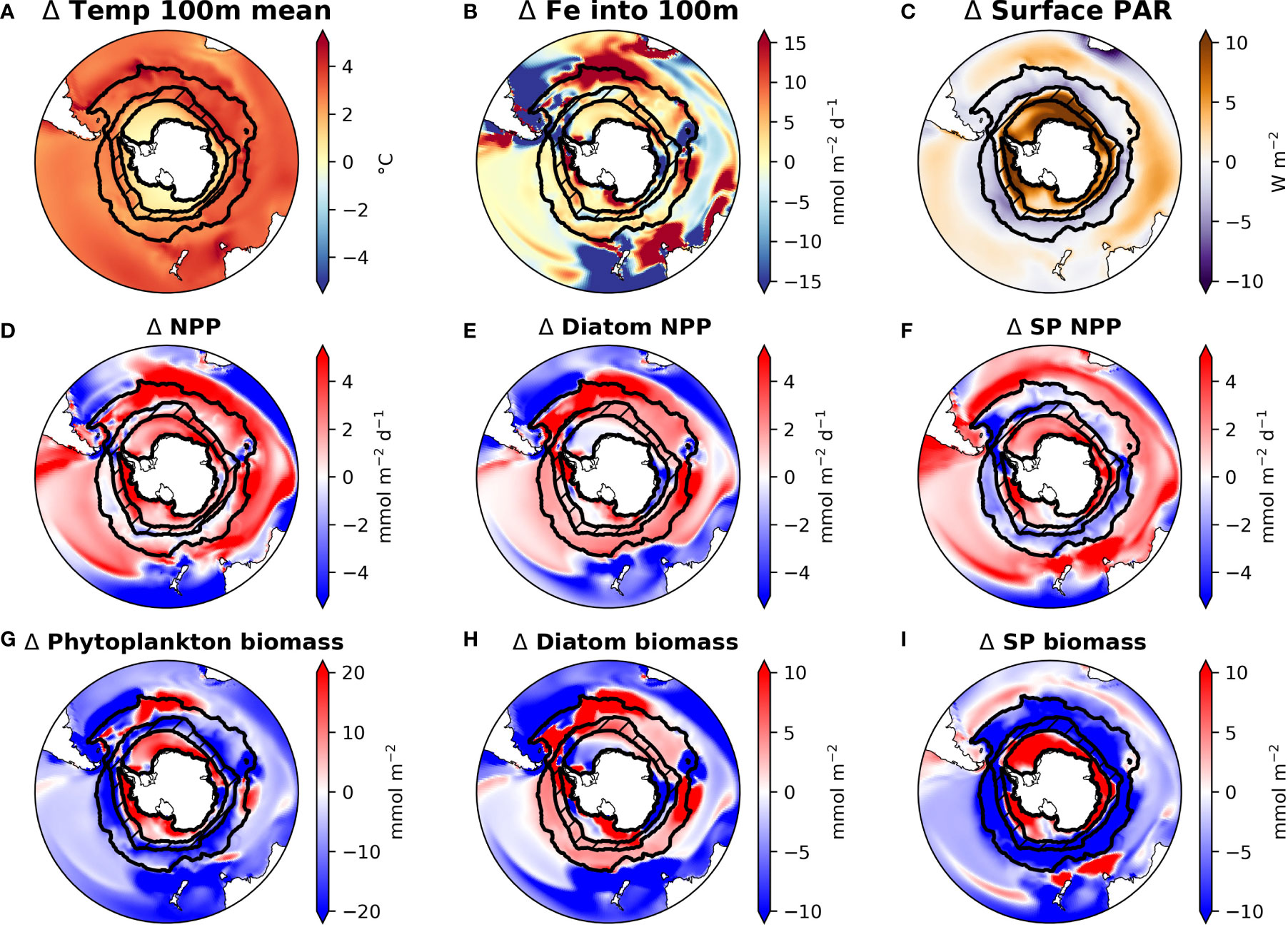
Figure 1 Maps of CESM1-LE ensemble mean changes from the 1920s to the 2090s in drivers (panels A–C) and phytoplankton production (panels D–F) and biomass (panels G–I) in the Southern Ocean. ACC and SIZ regions are shown by black contours, with the marginal SIZ hatched. Abbreviations: small phytoplankton (SP); temperature in top 100 m (temp 100m mean); physically-mediated flux of iron into the top 100m (Fe into 100m); photosynthetically active radiation (PAR); net primary production (NPP).

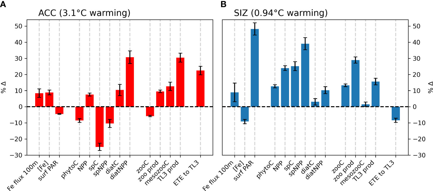
Figure 2 Percent changes in environmental drivers and biological responses that accompany climatic warming from the 1920s to the 2090s (CESM1-LE ensemble mean), in the (A) Antarctic Circumpolar Current (ACC) and (B) the sea ice zone (SIZ) regions of the Southern Ocean. Environmental drivers include depth-integrated horizontal and vertical fluxes over the top 100m (Fe flux 100m), top 100m mean iron concentration ([Fe]), and photosynthetically active radiation at the surface (surf PAR). Biomass terms include total phytoplankton biomass (phytoC), as well as small phytoplankton biomass (spC), diatom biomass (diatC), total zooplankton biomass (zooC), and mesozooplankton biomass (mesozooC). Production terms include total net primary production (NPP), small phytoplankton NPP (spNPP), diatom NPP (diatNPP), zooplankton production (zoo prod), and trophic level 3 production (TL3 prod). Ecosystem transfer efficiency to trophic level 3 is abbreviated “ETE to TL3”. All biomass and production terms are integrated over the top 100m. Error bars represent one standard deviation among ensemble members in the CESM1-LE, and thus show the influence of internal climate variability.

CESM simulates that, by the late 21st century, both the ACC and SIZ will have similar increases in physically-mediated iron flux into the top 100 m (Figure 2; see also Figure S5C for the change in vertical iron flux). Other nutrients also show similar changes in physically-mediated fluxes into the top 100 m (not shown), but here we focus on iron since it generally limits production in the Southern Ocean. The simulated change in the advective iron supply in the Southern Ocean is heterogeneous; for instance the western sector of the Atlantic basin shows intense reductions in supply, but these are compensated by increased supply in the east (Figure 1B). Despite this heterogeneity, the aggregate change in iron flux in the ACC is an increase by 2.3 nmol Fe m^-2d^-1, while in the SIZ iron flux increases by 2.4 nmol Fe m^-2d^-1 (+8.4% and +8.8%, respectively; Figure 2 and Table 2). There is, however, higher standard deviation among ensemble members for physically-mediated iron flux than other environmental drivers, especially in the SIZ (error bars on Figure 2), indicating that most the change is within the range of natural climate variability.

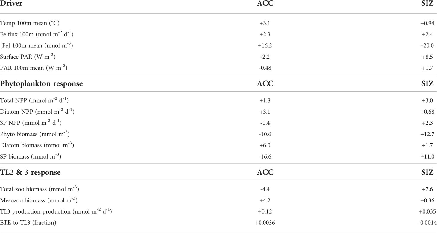
Table 2 CESM-LE ensemble mean changes in drivers, phytoplankton, and trophic level 2 (zooplankton) and 3 from the 1920s to the 2090s.

These changes in iron flux are likely due a combination of physical changes that occur with warming. These include wind-driven changes – zonal wind stress increases in many areas of the ACC and SIZ (Figure S5E), while meridional wind stress decreases in most regions, with the exception of the western sector of the Atlantic and some coastal areas of the SIZ (Figure S5F). These changes result in altered circulation patterns under RCP8.5 warming; mixed layer depth decreases in most areas of the Southern Ocean, with pockets of deeper mixed layer depths in the western sector of the Atlantic and around the edge of the SIZ (Figure S5D), further contributing to the heterogeneity of changes in iron flux. Other reasons for changing iron flux include water column destabilization with sea ice loss (Figure S5B) and unused iron advecting from the subtropics where productivity has dropped due to warming-induced ocean stratification.

Increasing iron input into the upper water column impacts phytoplankton growth in the Southern Ocean, where iron is generally limiting primary production. As such, we expect that 1) enhanced supply of iron could drive enhanced growth and that 2) a change in iron concentration would imply a change in the phytoplankton iron utilization fraction. Iron concentration in the ACC increases, reflecting increased iron input (Figures 2A and S5A) accompanied by a decreased utilization fraction. In the SIZ, however, the iron concentration actually decreases despite increasing iron flux (Figures 1B and 2B), indicating increases in productivity and iron utilization fraction in the SIZ. This is due to synchronous changes in light input, which offer phytoplankton in the SIZ more opportunity to draw down iron concentrations.

CESM-simulated changes in photosynthetically active radiation (PAR) arriving at the ocean surface are most dramatic in the SIZ (Figure 1C), where climatic warming leads to ~50% loss of sea ice around Antarctica. This sea ice decline results in an annual mean surface PAR increase of 8.5 W m^-2 in the SIZ (Table 2), a nearly 50% increase (Figure 2B). CESM also simulates a slight decrease in surface PAR in the ACC (Figures 1C, 2A) by 2.2 W m^-2 (-4.5%; Table 2). Here decreases in light are caused by increased cloudiness in this region as westerlies shift southward (Figure S5E). These changes in light along with the changes in iron supply, as described above, lead to interesting rearrangements of the phytoplankton communities in the light- and iron-limited Southern Ocean.

3.1.2 Phytoplankton community changes

CESM simulates increases in net primary productivity (NPP) by marine phytoplankton throughout the Southern Ocean under RCP8.5. The strongest increases in NPP occur in parts of the SIZ and around the northern flanks of the ACC in Atlantic and Indian sectors, while the weakest increases occur in the Pacific sector of the ACC (Figure 1D). These changes in NPP are further explained by examining the contributions by each phytoplankton functional type in the Southern Ocean. Diatom NPP increases in the ACC, while small phytoplankton NPP declines (Figures 1E, F, 2A; Table 2). Thus, the NPP increases in the ACC are entirely due to increases in diatom NPP. In the SIZ, on the other hand, overall diatom NPP increases by ∼10%, confined to areas along the Antarctic Peninsula and near the Ross Sea (Figure 1E). In contrast, small phytoplankton NPP increases are widespread in the SIZ, showing a ∼40% increase (Figure 2B). These extensive simulated increases in NPP are not necessarily accompanied by increases in phytoplankton biomass.

Total phytoplankton biomass declines in most areas outside of the SIZ, despite increasing productivity (Figure 1G), dropping by nearly 10% in the ACC (Figure 2A). Nearly all of this decline is due to losses of small phytoplankton biomass (Figure 1I, Table 2). In fact, the only place where total phytoplankton biomass increases in the ACC is in the eastern part of the Atlantic sector, where both iron inputs and diatom NPP increase strongly (Figures 1B, E, H). The reason for the increasing NPP in the ACC but decreasing biomass concerns the balance between phytoplankton sources and sinks: increased temperature and iron input stimulates phytoplankton productivity in the ACC, but losses, such as grazing and mortality also accelerate with warming (see Material and Methods). As such, losses slightly exceed growth under warming, leading to overall biomass reduction. Also worth noting, the ensemble member spread (i.e., internal variability) of small phytoplankton biomass in the ACC declines under RCP8.5 warming, indicating that interannual variability is dampened with climate change (Figure S6). Interestingly, this does not occur with diatom biomass in the ACC.

In contrast to the ACC, NPP increases in the SIZ are large enough to produce an increase in overall phytoplankton biomass. Most of the increase, however, is due to increases in small phytoplankton (Table 2); diatom biomass only increases slightly (∼3%; Figure 2B) and is limited to small pockets mainly along western Antarctica (Figures 1E, H). Such a strong increase in small phytoplankton NPP and biomass is driven by a decrease in light limitation from sea ice loss (Figure 1C), allowing small phytoplankton to compete more effectively with diatoms.

3.2 Changing ecosystem phenology

These CESM simulations indicate that, in the ACC, changes in annual mean phytoplankton community composition are associated with shifts in seasonality. During the 1920s, small phytoplankton abundance peaked in December, with diatoms having a smaller peak in biomass during February (Figures 3A, B). By the 2090s, the small phytoplankton bloom is reduced by ~70 mmol C m^-2 (Figure 3C) and small phytoplankton biomass peaks much earlier, in October. Diatoms, on the other hand, bloom a month earlier in the ACC, in January, by the end of the century, and gain nearly 50 mmol C m^-2 of biomass (Figures 3A–C). Standard deviation of CESM1-LE ensemble members is low around these changes in phytoplankton biomass indicating a strong climate change forced signal (shaded areas on Figures 3A–C); most variability among ensemble members is present during the height of the growing season. Overall, conditions during the ACC growing season appear to be more favorable for diatoms by the end of the century.

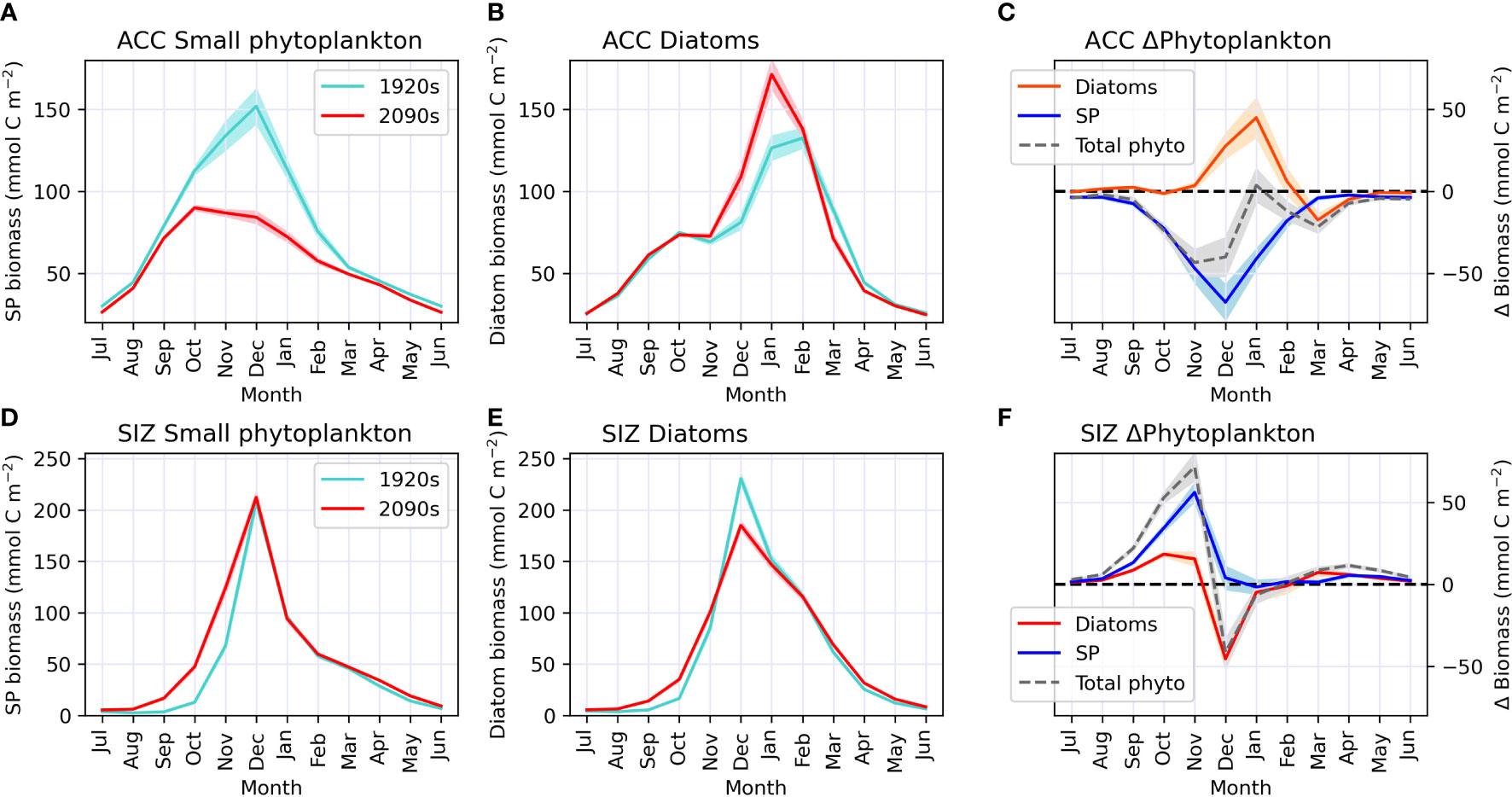
Figure 3 Monthly climatology (centered on Southern hemisphere summer) of biomass for each epoch during our study period (1920s and 2090s) for small phytoplankton (SP; panels A, D) and diatoms (panels B, E) in the Antarctic Circumpolar Current (ACC; top row) and sea ice zone (SIZ; bottom row). Panels C, F show phytoplankton biomass anomalies in the ACC and SIZ, respectively, for the 2090s relative to the 1920s for total phytoplankton (in gray dashed line), small phytoplankton (SP; in red) and diatoms (in blue); i.e. the red line minus the turquoise line from the plots on the left. Darker lines represent the CESM1-LE ensemble mean, while shading behind line represents one standard deviation among CESM1-LE ensemble members. Note that the standard deviation for panels (D, E) is so small it is nearly indistinguishable from the mean line.

In the SIZ, on the other hand, the timing of peak phytoplankton blooms does not change with climate warming (both diatoms and small phytoplankton continue to peak in biomass in December), despite earlier retreats in sea ice. However, these CESM1-LE simulations show advances in the onset of springtime productivity that ultimately affect the magnitude and composition of the December blooms (Figures 3D–F). By the 2090s, warming-induced sea ice declines cause small phytoplankton to start gaining biomass earlier in the growing season, gaining ∼30 mmol C m^-2 and > 50 mmol C m^-2 in October and November, respectively (Figure 3F). Diatoms, on the other hand, slightly gain biomass during these early months of the growing season, but then drop in biomass by ~50 mmol C m^-2 in December (Figures 3E, F). This reduction of diatom biomass during the peak growing season is caused by a depletion of nutrients (iron) from phytoplankton growth in the spring. Thus, the earlier springtime sea ice retreat by the 2090s in CESM causes modifications to phytoplankton production and community composition over the entire growing season. These phytoplankton changes in the SIZ are similar among all CESM1-LE ensemble members, as there is very little standard deviation around these changes (shaded areas on Figures 3D–F).

In summary, these climate change simulations indicate that diatoms may proliferate and bloom earlier in the ACC region while, in the SIZ, small phytoplankton could start growing earlier and reduce the magnitude of the peak diatom bloom. These shifts in phytoplankton community composition in these two regions of the Southern Ocean are driven by a combination of warming and changes in light and nutrient concentrations. In the following section we analyze how changes in environmental conditions induce such community shifts.

3.3 Drivers of change: A resource competition perspective

We further explore how concurrent changes in bottom up drivers of phytoplankton in the Southern Ocean could alter phytoplankton community composition from a resource competition perspective (Tilman, 1977). In the ACC, simulated changes in environmental conditions under RCP8.5 support increases in diatoms. The 3.1°C increase in top 100m mean temperature along with a slight decrease in irradiance drive a shift to higher diatom growth rates relative to small phytoplankton (indicated by an arrow on Figure 4A). Though diatoms and small phytoplankton have the same temperature limitation parameterization, the temperature-dependent growth rate in the light limitation equation (see Material and Methods) produces more favorable conditions for diatoms, especially under low light conditions. A higher maximum chlorophyll to carbon ratio in diatoms (Figure S1; see Material and Methods), allowing for greater photoadaptation, is also important in the direction of this phytoplankton shift. This is also evident in PAR versus iron resource competition space for the ACC (Figure 4C), where slightly lower light along with higher iron concentrations induces a shift to conditions where diatoms have faster growth rates relative to small phytoplankton. Thus, both resource competition plots for the ACC (Figures 4A, C) show shifts to bottom up environmental conditions that would favor diatoms, explaining why the model shows increasing diatom prevalence in this region.

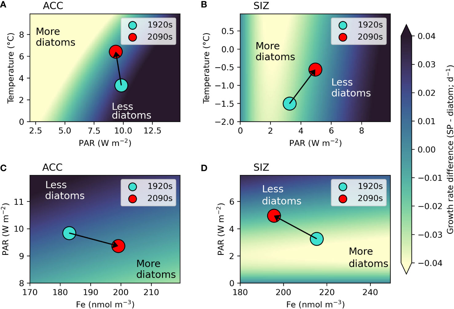
Figure 4 Resource competition plots. Panels A, B show the difference between small phytoplankton (SP) and diatom growth rates (SP - diatom) in temperature (T) and light (as photosynthetically active radiation; PAR) space for the Antarctic circumpolar current (ACC) and sea ice zone (SIZ), respectively. Panels C, D show the same growth rate difference, but in iron (Fe) concentration and PAR space for the ACC and SIZ, respectively. For the T versus PAR plots, growth rates were calculated using 2090s top 100m Fe concentrations for each region, while for the PAR versus Fe plots growth rates were calculated using 2090s 100m mean T for each region. Top 100m mean annual values for each environmental variable and region are shown by dots for each epoch: 1920s (turquoise dots) to 2090s (red dots). Arrows show direction of change from the 1920s to 2090s, showing how the regions shift to having more (or less) diatoms. Axes were adjusted to focus on relevant ranges of each environmental variable for each region. Lighter colors indicate more ideal conditions for diatom growth (i.e. diatom growth rates are faster than those of small phytoplankton).

By contrast, environmental changes in the SIZ work against diatoms. The SIZ warms by 0.94^°C with more dramatic increases in light (an increase of 1.7 W m^-2 over the top 100m and 8.5 W m^-2 at the surface; Figures 4B, D and Table 2). Though the total flux of iron into the top 100m of the SIZ increases (Figures 1B, 2B, and Table 2), the iron concentration decreases, as shown by the direction of the arrow on Figure 4D. This illustrates the synergistic effect of increasing light and iron flux: as light increases, the ability of phytoplankton to make use of available iron also increases and overall iron concentration declines. Since small phytoplankton are more competitive for iron at low concentrations (i.e., they have a lower iron half saturation constant for iron uptake in the model), this moves the SIZ into conditions that select for more small phytoplankton (and fewer diatoms) by the 2090s (Figure 4D). Shifts of this nature at the base of the food web could have ramifications for higher trophic levels.

3.4 Implications for higher trophic levels

Aside from one generic zooplankton class, the CESM1 does not explicitly simulate higher trophic levels. Therefore we used established methods for estimating potential effects of these simulated CESM1-LE phytoplankton community shifts on trophic levels 2 (i.e., herbivorous zooplankton) and 3 (i.e., organisms that consume herbivorous zooplankton, such as fish). Overall zooplankton biomass declines over much of the Southern Ocean, only increasing in the SIZ (Figure 5A). In contrast, estimated mesozooplankton biomass increases throughout the ACC, reflective of increases in diatom abundance there (Figure 5B). The SIZ shows regionally variable changes in mesozooplankton biomass, increasing around the Antarctic Peninsula and Ross Sea regions, but decreasing in all other areas in the SIZ.

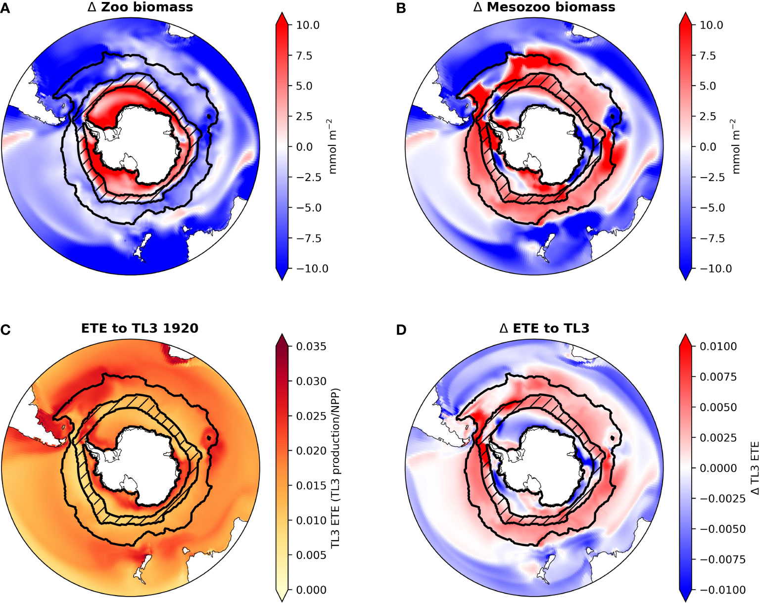
Figure 5 Maps of CESM-LE ensemble mean changes from the 1920s to the 2090s in total zooplankton biomass (A), mesozooplankton biomass (B) and ecosystem transfer efficiency (ETE) to trophic level 3 (TL3) for the 1920s (C) and the CESM-LE ensemble mean change in ETE to TL3 from the 1920s to the 2090s (D) in the Southern Ocean. ACC and SIZ regions are shown black contours, with the marginal SIZ hatched.

Following Moore et al. (2018), we estimated pelagic TL3 production using the method of Stock et al. (2017) (see Material and Methods and Equation 7); in the Southern Ocean this could be representative of the growth of whales, penguins, seals, or some fish species (e.g., Antarctic silver fish). TL3 production shows widespread increases by the 2090s, mostly as a result of increasing mesozooplankton production (Figure S7). However, despite increasing NPP and phytoplankton biomass in the SIZ, TL3 production in most areas of the SIZ barely changes. This is because the increases in primary production are mainly confined to small phytoplankton, which do not contribute to our estimation of mesozooplankton biomass and production. TL3 production, however, increases in the ACC, especially in the Atlantic sector.

Ecosystem transfer efficiency (ETE) describes how efficiently NPP is transferred to higher trophic level production. Here, we estimated ETE to TL3. In the 1920s ETE in CESM ranged from ∼ 0.01 to 0.035 in most regions of the Southern Ocean (Figure 5C). By the 2090s ETE increases in all areas of the ACC by roughly 0.005 to 0.01 (a ∼22% increase). ETE changes are spatially variable in the SIZ (Figure 5D): ETE in most parts of the SIZ decreases (overall a decline of ∼8%; Figure 2B), but ETE along the Antarctic Peninsula and near the Ross Sea increases slightly; these are the few areas of the SIZ where mesozooplankton biomass also increases with climate change (Figure 5B).

4 Discussion

In this study, we document how anthropogenic climate may drive changes in Southern Ocean phytoplankton communities with ramifications for Antarctic food chains. Despite the simplistic nature of the ecosystem model in CESM, climate-induced changes in the ACC and SIZ are enough to produce shifts in the balance between two major phytoplankton functional types with differing strategies for growth and resource acquisition. Using the terminology from Dutkiewicz et al. (2013), the “opportunist” strategy of diatoms becomes more successful in the ACC and the “gleaner” strategy of small phytoplankton becomes more advantageous in the SIZ (Figure 6). Warming, increased iron concentrations, and less light drive phytoplankton rearrangements in the ACC. In the SIZ, increases in light drive increased iron utilization and shift environmental conditions to those that favor small phytoplankton. These environmental change projections are generally in agreement with other studies (Leung et al., 2015; also see a review by Henley et al., 2020). Not only do these changes impact the biological carbon pump (Figure S8), but they also proliferate up the food web, setting up potential shifts in prey resources for Antarctic marine predators.

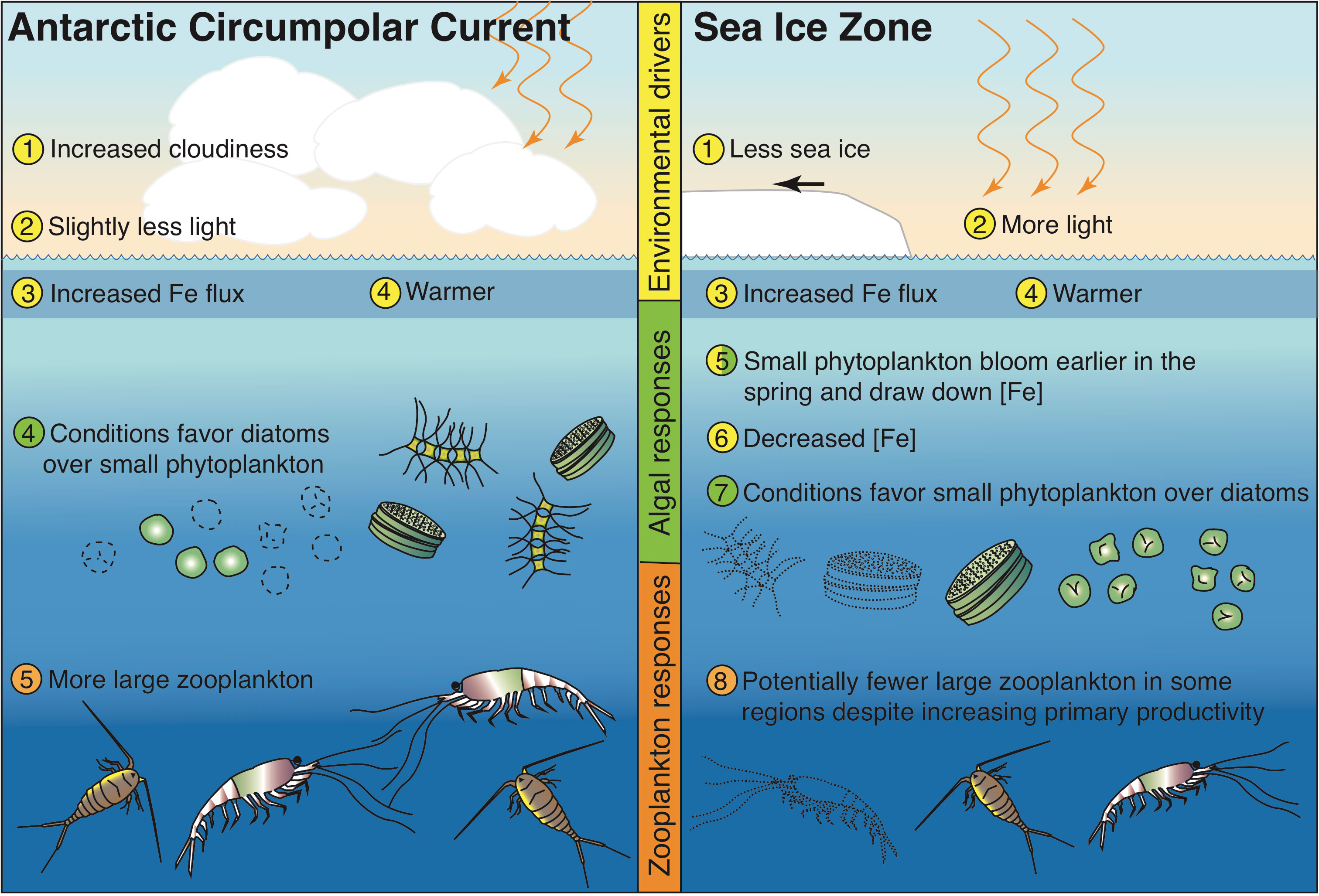
Figure 6 Schematic of hypothesized changes to Southern Ocean ecosystem in the Antarctic Circumpolar Current region and the Sea Ice Zone, based on the results of the CESM1-LE under a high emission scenario.

The nature of the simulated changes described here and summarized in Figure 6 hinge on the dynamics of a few key model parameterizations. Geider’s light physiology and photoadaptation model (Geider et al., 1997) describes how phytoplankton growth adapts to changing light levels in the context of temperature and nutrient availability. A critical part of this parameterization is the variable chlorophyll to carbon ratios, which increase under low light conditions; higher maximum carbon to chlorophyll ratios in diatoms confer an advantage under decreasing light (e.g., Figure S1; Table 1; Geider et al., 1997). Thus, in these CESM simulations, diatoms compete more effectively under decreased light and increased temperature in the ACC under future warming and small phytoplankton proliferate more than diatoms with increased light in the SIZ as sea ice cover declines. Another key parameterization is Monod nutrient uptake kinetics with smaller half saturation constants for nutrients for small phytoplankton than for diatoms; a boost in iron concentrations in the ACC (Figures 2A, 4) causes diatom growth rates to increase more than small phytoplankton growth rates because small phytoplankton are closer to saturation with respect to iron uptake than diatoms. The opposite happens in the SIZ, where diatom growth is hindered more by declining iron concentrations than small phytoplankton growth. These light and nutrient uptake parameterizations are common in major Earth system models (Laufkötter et al., 2015).

The environmental and biological changes to the Southern Ocean simulated here are mainly consistent with other Coupled Model Intercomparison Project (CMIP) class models under high emission scenarios. Multiple climate models have projected a poleward contraction of the westerly wind belt associated with an increasingly positive Southern Annular Mode (SAM) under anthropogenic climate change (Arblaster and Meehl, 2006; Simpson and Polvani, 2016; Kajtar et al., 2021). Accompanying the movement of this jet, is the poleward increase in cloudiness and associated decrease in light in the ACC region of the Southern Ocean. Increased cloudiness in the Southern Ocean with climate change was shown by Leung et al. (2015) for an ensemble of models, dropping summertime PAR by 12 to 18 W m^-2 between ∼45°S and 60°S (larger than is shown here for the CESM1-LE ensemble mean in the ACC region; Table 2). Increasing light penetration in the SIZ due to sea ice loss is also common among CMIP class models (Leung et al., 2015; Roach et al., 2020). Also influencing light availability for phytoplankton is mixed layer depth (MLD), with deeper mixed layers invoking more light limitation. While the CESM1-LE and CMIP6 models do not show an overall increase in MLD in the Southern Ocean (Figure S5D; Kwiatkowski et al., 2020), other CMIP5 models did (Leung et al., 2015). Leung et al. (2015) also showed a general increase in winter iron concentration in CMIP5 models as intensified westerlies increase upwelling of iron to surface layers, consistent with the overall increasing iron flux in the ACC and SIZ (Figures 1B, 2; Table 2). Phytoplankton responses to climate change in the Southern Ocean also agree. In a CCSM (Community Climate System Model, a previous version of CESM) simulation run under a high emission scenario, diatom growth rates increased in the subpolar region of the Southern Ocean (Marinov et al., 2010), as did diatom productivity in simulations with the latest version of CESM (CESM version 2; Long et al., 2021).

Despite short observational records in the Southern Ocean, some studies have captured trends in Southern Ocean diatoms that match the trends in diatoms hypothesized here under climatic warming. Using a satellite product for diatom specific chlorophyll, Soppa et al. (2016) showed that diatom bloom chlorophyll maxima have been increasing in the Subantarctic Southern Ocean from 1997 to 2012. Likewise, over the same time period, Rousseaux and Gregg (2015) used an ocean circulation model in combination with ocean color data assimilation to derive trends in various phytoplankton groups; diatoms in this study increased significantly in parts of the ACC region, between ∼45°S to 60°S, and decreased along the Antarctic continent. This study also noted a decrease in diatom abundance south of 60°S (except the Weddell Sea), similar to the relative decrease in diatom abundance in the SIZ in this study (Figure 3F). Thus, these relatively short timeseries lend support for the longer term changes in diatoms shown here by the CESM1-LE. However, the observational record is generally too short to capture long term trends apart from natural variability (Henson et al., 2016).

These CESM1 simulations show that the diatom response to climate change is spatially variable within the SIZ, with two locations showing diatom increases: The Antarctic Peninsula and the Ross Sea. Higher diatom productivity in these regions flows up the food chain, leading to more mesozooplankton and slightly higher ETE (Figures 5B, D). Sea ice declines and surface PAR increases are fairly uniform throughout the SIZ (Figures S5B, C). Iron is the likely reason behind the diatom increase in these particular areas of the SIZ. These areas show particularly high increased iron input into the top 100m (Figure 1B), which results in tiny pockets of increased iron concentrations, despite the longer growing season that offers phytoplankton more chance to draw down the iron (Figure S5A). This demonstrates how subtle regional shifts in environmental conditions may be important to determining shifts in the dominant phytoplankton ecological strategy.

The changes in diatom abundance in the Southern Ocean modeled here would affect major zooplankton species, such as copepods and krill. Antarctic krill (Euphausia superba) are one of the most important zooplankton in the Southern Ocean, providing a link between primary production and marine predators, such as whales and penguins (Smetacek, 2008; Henley et al., 2020). Changes in estimated mesozooplankton biomass in these CESM1-LE simulations suggest increases in zooplankton species like E. superba in the ACC and declines in the SIZ. While Antarctic krill have been shown to select for diatoms over small phytoplankton (Haberman et al., 2003; Moline et al., 2004), they can have a more diverse diet that includes small zooplankton like flagellates and tintinnids, in addition to diatoms (Schmidt et al., 2006). Overall increases in productivity and a phytoplankton community shift in the SIZ towards more small phytoplankton (and a decreasing proportion of diatoms) could favor zooplankton species that prefer a diet that includes more microzooplankton. Another key krill species in the Southern Ocean, Thysanoessa macrura, may more actively switch to a carnivorous diet than E. superba (Yang et al., 2021); this species is also expected to have increased growth rates under climatic warming (Driscoll et al., 2015). More small phytoplankton in the SIZ could also cause krill to be out-competed by salps, which are better at grazing small organisms (e.g., see Moline et al., 2004); salps are not the preferred food source for higher level organisms (like penguins and seals). In any case, Antarctic krill populations could be negatively impacted by the loss of sea ice from climatic warming, as the major limiting factor for successful larval krill recruitment is the seasonal location of sea ice (Ryabov et al., 2017; Thorpe et al., 2019). Low sea ice in combination with reduced diatom biomass could lead to less successful krill cohorts.

Changes in the amount of secondary producers (e.g., mesozooplankton in Figure 5B) could impact trophic level 3 organisms (Figure 5C) and will depend on the interaction between changes to temperature, transfer efficiency, and food chain length. Rising temperatures would foster higher growth rates in ectotherms, like fish, as long as they are able to meet their basal metabolic demands. According to the model results shown here, greater fish biomass could be likely in the ACC where temperature, NPP, and diatom biomass all increase (Figure 1), leading to more mesozooplankton and TL3 productivity (Figures 5B, S5). The impact of lower ecosystem level changes simulated in this study for the SIZ is more complex, as productivity increases but so does the proportion of small phytoplankton. An increasing fraction of small phytoplankton could result in losses to energy transfer due to longer food chains. Production by small phytoplankton tends to be more recycled, cycling energy within the microbial loop rather than up the food chain (Sommer et al., 2002). Further, a biogeographical shift of diatoms and their zooplankton predators away from the SIZ northward towards the ACC, could cause Antarctic predators to travel further to consume prey and return it to their young during the breeding season. This, in combination with declining sea ice, could cause population declines in species such as the Emperor penguin (Jenouvrier et al., 2014).

The reproductive success of Southern Ocean marine predators would not only be impacted by the spatial distribution of phytoplankton and zooplankton, but also by the seasonal timing of their blooms. Despite some model biases in the timing of the blooms (Figure S2), these CESM1-LE results show that phytoplankton may change the seasonal timing of their blooms in the Southern Ocean, with diatoms blooming a month earlier in the ACC and small phytoplankton starting to grow earlier in the SIZ (reducing peak diatom blooms in December). While the generic zooplankton type in CESM consumes phytoplankton regardless of bloom timing, actual Antarctic zooplankton species may not be so flexible. Phenology of high latitude organisms has evolved to exploit the most favorable periods of the year for growth and reproduction; animals often time breeding in response to temperature and/or light (Ji et al., 2010; Asch et al., 2019). If phytoplankton blooms occur before zooplankton populations are sufficiently large to graze them down, more production may be exported out of the pelagic ecosystem, reducing flow of biomass to top predators. Mismatch in phenology would be further complicated by changing sea ice cover in the Antarctic SIZ, which is necessary for krill (Meyer et al., 2009) and many sea birds (Jenouvrier et al., 2014; Iles et al., 2020) and marine mammals (Bester et al., 2017). In short, the basic rearrangements of phytoplankton communities shown here for the CESM1-LE under climate change could have a multitude of cascading consequences for Antarctic ecosystems.

The phytoplankton community shifts and potential impacts on higher trophic levels hypothesized in this study have numerous caveats. Most obviously, the marine ecosystem in CESM is highly simplistic and parameters describing phytoplankton groups are generally tuned to capture global distributions of functional groups. We further rely on scaling relationships to partition zooplankton biomass, estimate trophic level 3 productivity, and calculate ETE. Using an Earth system model with better resolved polar algal groups (e.g., Phaeocystis; Wang et al., 2015), as well as zooplankton groups (e.g., Antarctic krill; Karakuş et al., 2021), would offer improved projections of how lower trophic levels in the Southern Ocean may respond to climate change. Furthermore, CESM, like most Earth system models, does not simulate the potential for evolutionary adaptation of phytoplankton under rapidly changing environmental conditions. This phenomenon has been demonstrated in several laboratory studies (Lohbeck et al., 2014; Padfield et al., 2016; Bach et al., 2018), where phytoplankton have adapted to warmer conditions or ocean acidification, achieving similar growth as in control conditions after as little as 100 generations (Padfield et al., 2016). While these intricacies are not considered here, our results do broadly demonstrate contrasting shifts in large scale ecological strategies in a biogeochemically and ecologically important region.

5 Conclusion

Here, we present a possible trajectory of how phytoplankton community composition may change in the Southern Ocean under a high emission anthropogenic warming scenario. These shifts in primary producers may impact the rest of the Antarctic food web through trophic connections. Warming, along with changes in light and iron concentrations in the ACC and SIZ in the Southern Ocean impact generalized phytoplankton physiology prescribed in the Earth system model. Simplistic groupings of small phytoplankton versus diatoms offer a springboard for further refinement. The wide diversity of life history strategies, growth rates, and temperature preferences in Antarctic phytoplankton and zooplankton may dampen or amplify the changes outlined in this study. As the Antarctic environment transitions rapidly in the coming decades under climate change, understanding restructuring of the base of the food chain is critical for forecasting potential shifts in food resources for Antarctic marine predators.

6 Permission to reuse and copyright

Figures, tables, and images will be published under a Creative Commons CC-BY licence and permission must be obtained for use of copyrighted material from other sources (including re-published/adapted/modified/partial figures and images from the internet). It is the responsibility of the authors to acquire the licenses, to follow any citation instructions requested by third-party rights holders, and cover any supplementary charges.

Data availability statement

Publicly available datasets were analyzed in this study. This data can be found here: CESM ensemble output is available from the Earth System Grid (https://www.earthsystemgrid.org/dataset/ucar.cgd.ccsm4.cesmLE.html). Analysis code for this study can be found in a public repository on GitHub [https://github.com/kristenkrumhardt/CESM1-LE-SO-diatoms].

Author contributions

KK and ML designed the study. ML helped with data processing and advised KK on analysis. KK did the analysis, made the figures, and wrote the first draft of the study. ZS aided in background research, writing, and analyzed zooplankton data. CP helped with interpretation of impacts on higher trophic levels and with writing the Introduction and Discussion. All authors revised and structured the manuscript. All authors contributed to the article and approved the submitted version.

Funding

Funding for this research was provided by NASA (Grant number 80NSSC20K1289, Project number 19-IDS19-0028) and NOAA (Grant numbers NA20OAR4310444, NA20OAR4310441 and NA20OAR4310442).

Acknowledgments

We thank members of the NASA-funded “Antarctic marine predators in a dynamic climate” project team for guidance and inspiration on this modeling study. We acknowledge high-performance computing support from Cheyenne (doi:10.5065/D6RX99HX) provided by NCAR’s Computational and Information Systems Laboratory, sponsored by the National Science Foundation. This material is based upon work supported by the National Center for Atmospheric Research, which is a major facility sponsored by the National Science Foundation under Cooperative Agreement No. 1852977

Conflict of interest

The authors declare that the research was conducted in the absence of any commercial or financial relationships that could be construed as a potential conflict of interest.

Publisher’s note

All claims expressed in this article are solely those of the authors and do not necessarily represent those of their affiliated organizations, or those of the publisher, the editors and the reviewers. Any product that may be evaluated in this article, or claim that may be made by its manufacturer, is not guaranteed or endorsed by the publisher.

Supplementary material

The Supplementary Material for this article can be found online at: https://www.frontiersin.org/articles/10.3389/fmars.2022.916140/full#supplementary-material

References

Arblaster J. M., Meehl G. A. (2006). Contributions of external forcings to southern annular mode trends. J. Climate 19, 2896–2905. doi: 10.1002/2016GL072428
Ardyna M., Claustre H., Sallée J-B., D'Ovidio F., Gentili B., van Dijken G., et al (2017). Delineating environmental control of phytoplankton biomass and phenology in the Southern Ocean. Geophysical Research Letters. 44 (10), 5016–5024. doi: 10.1002/2016GL072428
Armengol L., Calbet A., Franchy G., Rodríguez-Santos A., Hernández-León S. (2019). Planktonic food web structure and trophic transfer efficiency along a productivity gradient in the tropical and subtropical atlantic ocean. Sci. Rep. 9, 2044. doi: 10.1038/s41598-019-38507-9
Asch R. G., Stock C. A., Sarmiento J. L. (2019). Climate change impacts on mismatches between phytoplankton blooms and fish spawning phenology. Global Change Biol. 25, 2544–2559. doi: 10.1111/gcb.14650
Bach L. T., Lohbeck K. T., Reusch T. B. H., Riebesell U. (2018). Rapid evolution of highly variable competitive abilities in a key phytoplankton species. Nat. Ecol. Evol. 2, 611–613. doi: 10.1038/s41559-018-0474-x
Bester M. N., Bornemann H., McIntyre T. (2017). Antarctic Marine mammals and sea ice (John Wiley & sons, Ltd), chap 22, 534–555. doi: 10.1002/9781118778371.ch22
Blain S., Quéguiner B., Armand L., Belviso S., Bombled B., Bopp L., et al. (2007). Effect of natural iron fertilization on carbon sequestration in the southern ocean. Nature 446, 1070–1074. doi: 10.1038/nature05700
Bopp L., Resplandy L., Orr J. C., Doney S. C., Dunne J. P., Gehlen M., et al. (2013). Multiple stressors of ocean ecosystems in the 21st century: projections with CMIP5 models. Biogeosciences 10, 6225–6245. doi: 10.5194/bg-10-6225-2013
Boyd P. W. (2019). Physiology and iron modulate diverse responses of diatoms to a warming southern ocean. Nat. Climate Change 9, 148–152. doi: 10.1038/s41558-018-0389-1
Chisholm S. W. (1992). Phytoplankton size (Boston, MA: Springer US), chap. Phytoplank. Siz. 43:213–237. doi: 10.1007/978-1-4899-0762-2{\_}12
Deppeler S. L., Davidson A. T. (2017). Southern ocean phytoplankton in a changing climate. Front. Mar. Sci. 4. doi: 10.3389/fmars.2017.00040
Deser C., Lehner F., Rodgers K. B., Ault T., Delworth T. L., DiNezio P. N., et al. (2020). Insights from earth system model initial-condition large ensembles and future prospects. Nat. Climate Change 10, 277–286. doi: 10.1038/s41558-020-0731-2
Driscoll R. M., Reiss C. S., Hentschel B. T. (2015). Temperature-dependent growth of thysanoessa macrura: inter-annual and spatial variability around elephant island, antarctica. Mar. Ecol. Prog. Ser. 529, 49–61.
Dutkiewicz S., Scott J. R., Follows M. J. (2013). Winners and losers: Ecological and biogeochemical changes in a warming ocean. Global Biogeochem. Cycle. 27, 463–477. doi: 10.1002/gbc.20042 Dutkiewicz:2013
Eddy T. D., Bernhardt J. R., Blanchard J. L., Cheung W. W., Colléter M., du Pontavice H., et al. (2021). Energy flow through marine ecosystems: Confronting transfer efficiency. Trends Ecol. Evol. 36, 76–86. doi: 10.1016/j.tree.2020.09.006
Feng Y., Hare C., Rose J., Handy S., DiTullio G., Lee P., et al. (2010). Interactive effects of iron, irradiance and co2 on ross sea phytoplankton. Deep. Sea. Res. Part I.: Oceanogr. Res. Paper. 57, 368–383. doi: 10.1016/j.dsr.2009.10.013
Ferreira A., Costa R. R., Dotto T. S., Kerr R., Tavano V. M., Brito A. C., et al. (2020). Changes in phytoplankton communities along the northern antarctic peninsula: Causes, impacts and research priorities. Front. Mar. Sci. 7. doi: 10.3389/fmars.2020.576254
Freeman N. M., Lovenduski N. S., Munro D. R., Krumhardt K. M., Lindsay K., Long M. C., et al. (2018). The variable and changing southern ocean silicate front: Insights from the cesm large ensemble. Global Biogeochem. Cycle. 32, 752–768. doi: 10.1029/2017GB005816
Garnesson P., Mangin A., Fanton d’Andon O., Demaria J., Bretagnon M. (2019). The CMEMS GlobColour chlorophyll α product based on satellite observation: multi-sensor merging and flagging strategies. Ocean. Sci. 15, 819–830. doi: 10.5194/os-15-819-2019
Geider R. J., MacIntyre H. L., Kana T. M. (1997). Dynamic model of phytoplankton growth and acclimation: responses of the balanced growth rate and the chlorophyll a:carbonratio to light, nutrient-limitation and temperature. Mar. Ecol. Prog. Ser. 148, 187–200.
Grise K. M., Polvani L. M., Tselioudis G., Wu Y., Zelinka M. D. (2013). The ozone hole indirect effect: Cloud-radiative anomalies accompanying the poleward shift of the eddy-driven jet in the southern hemisphere. Geophys. Res. Lett. 40, 3688–3692. doi: 10.1002/grl.50675
Haberman K. L., Ross R. M., Quetin L. B. (2003). Diet of the antarctic krill (euphausia superba dana): Ii. selective grazing in mixed phytoplankton assemblages. J. Exp. Mar. Biol. Ecol. 283, 97–113. doi: 10.1016/S0022-0981(02)00467-7
Hansen P. J., Bjørnsen P. K., Hansen B. W. (1997). Zooplankton grazing and growth: Scaling within the 2-2,-μm body size range. Limnol. Oceanogr. 42, 687–704. doi: 10.4319/lo.1997.42.4.0687
Hasselmann K. (1976). Stochastic climate models part i. Theory. Tellus. 28, 473–485. doi: 10.1111/j.2153-3490.1976.tb00696.x
Hellessey N., Johnson R., Ericson J. A., Nichols P. D., Kawaguchi S., Nicol S., et al. (2020). Antarctic Krill lipid and fatty acid content variability is associated to satellite derived chlorophyll a and Sea surface temperatures. Sci. Rep. 10, 6060. doi: 10.1038/s41598-020-62800-7
Heneghan R. F., Galbraith E., Blanchard J. L., Harrison C., Barrier N., Bulman C., et al. (2021). Disentangling diverse responses to climate change among global marine ecosystem models. Prog. Oceanogr. 198:102659
Henley S. F., Cavan E. L., Fawcett S. E., Kerr R., Monteiro T., Sherrell R. M., et al. (2020). Changing biogeochemistry of the southern ocean and its ecosystem implications. Front. Mar. Sci. 7. doi: 10.3389/fmars.2020.00581
Henson S. A., Beaulieu C., Lampitt R. (2016). Observing climate change trends in ocean biogeochemistry: when and where. Global Change Biol. 22, 1561–1571. doi: 10.1111/gcb.13152
Hunt B. P., Espinasse B., Pakhomov E. A., Cherel Y., Cotté C., Delegrange A., et al. (2021). Pelagic food web structure in high nutrient low chlorophyll (hnlc) and naturally iron fertilized waters in the kerguelen islands region, southern ocean. J. Mar. Syst. 103625. doi: 10.1016/j.jmarsys.2021.103625
Iles D. T., Lynch H., Ji R., Barbraud C., Delord K., Jenouvrier S. (2020). Sea Ice predicts long-term trends in adélie penguin population growth, but not annual fluctuations: Results from a range-wide multiscale analysis. Global Change Biol. 26, 3788–3798. doi: 10.1111/gcb.15085
Jenouvrier S., Holland M., Stroeve J., Serreze M., Barbraud C., Weimerskirch H., et al. (2014). Projected continent-wide declines of the emperor penguin under climate change. Nat. Climate Change 4, 715–718. doi: 10.1038/nclimate2280
Ji R., Edwards M., Mackas D. L., Runge J. A., Thomas A. C. (2010). Marine plankton phenology and life history in a changing climate: current research and future directions. J. Plank. Res. 32, 1355–1368. doi: 10.1093/plankt/fbq062
Kajtar J. B., Santoso A., Collins M., Taschetto A. S., England M. H., Frankcombe L. M. (2021). Cmip5 intermodel relationships in the baseline southern ocean climate system and with future projections. Earth’. Future 9, e2020EF001873. doi: 10.1029/2020EF001873
Karakuş O., Völker C., Iversen M., Hagen W., Wolf-Gladrow D., Fach B., et al. (2021). Modeling the impact of macrozooplankton on carbon export production in the southern ocean. J. Geophys. Res.: Ocean. 126, e2021JC017315. doi: 10.1029/2021JC017315
Kay J. E., Deser C., Phillips A., Mai A., Hannay C., Strand G., et al. (2015). The community earth system model (CESM) large ensemble project: A community resource for studying climate change in the presence of internal climate variability. Bull. Am. Meteorol. Soc. 96, 1333–1349. doi: 10.1175/BAMS-D-13-00255.1
Kelleher M. K., Grise K. M. (2021). Varied midlatitude shortwave cloud radiative responses to southern hemisphere circulation shifts. Atmos. Sci. Lett., e1068. doi: 10.1002/asl.1068
Krumhardt K. M., Long M. C., Lindsay K., Levy M. N. (2020). Southern ocean calcification controls the global distribution of alkalinity. Global Biogeochem. Cycle. 34, e2020GB006727. doi: 10.1029/2020GB006727
Krumhardt K. M., Lovenduski N. S., Long M. C., Lindsay K. (2017). Avoidable impacts of ocean warming on marine primary production: Insights from the CESM ensembles. Global Biogeochem. Cycle. 31, 114–133. doi: 10.1002/2016GB005528
Kwiatkowski L., Torres O., Bopp L., Aumont O., Chamberlain M., Christian J. R., et al. (2020). Twenty-first century ocean warming, acidification, deoxygenation, and upper-ocean nutrient and primary production decline from cmip6 model projections. Biogeosciences 17, 3439–3470. doi: 10.5194/bg-17-3439-2020
Laufkötter C., Vogt M., Gruber N., Aita-Noguchi M., Aumont O., Bopp L., et al. (2015). Drivers and uncertainties of future global marine primary production in marine ecosystem models. Biogeosciences 12, 6955–6984. doi: 10.5194/bg-12-6955-2015
Leung S., Cabré A., Marinov I. (2015). A latitudinally banded phytoplankton response to 21st century climate change in the southern ocean across the CMIP5 model suite. Biogeosciences 12, 5715–5734. doi: 10.5194/bg-12-5715-2015
Lima D. T., Moser G. A. O., Piedras F. R., Cunha L. C. D., Tenenbaum D. R., Tenório M. M. B., et al. (2019). Abiotic changes driving microphytoplankton functional diversity in admiralty bay, king george island (antarctica). Front. Mar. Sci. 6. doi: 10.3389/fmars.2019.00638
Lohbeck K. T., Riebesell U., Reusch T. B. H. (2014). Gene expression changes in the coccolithophore emiliania huxleyi after 500 generations of selection to ocean acidification. Proc. R. Soc. B.: Biol. Sci. 281, 1–7.
Long M. C., Deutsch C., Ito T. (2016). Finding forced trends in oceanic oxygen. Global Biogeochem. Cycle. 30, 381–397. doi: 10.1002/2015GB005310
Long M. C., Lindsay K., Peacock S., Moore J. K., Doney S. C. (2013). Twentieth-century oceanic carbon uptake and storage in CESM1(BGC). J. Climate 26, 6775–6800. doi: 10.1175/JCLI-D-12-00184.1
Long M. C., Moore J. K., Lindsay K., Levy M., Doney S. C., Luo J. Y., et al. (2021). Simulations with the marine biogeochemistry library (marbl). J. Adv. Model. Earth Syst. 13, e2021MS002647. doi: 10.1029/2021MS002647
Lovenduski N. S., McKinley G. A., Fay A. R., Lindsay K., Long M. C. (2016). Partitioning uncertainty in ocean carbon uptake projections: Internal variability, emission scenario, and model structure. Global Biogeochem. Cycle. 30, 1276–1287. doi: 10.1002/2016GB005426
Marinov I., Doney S. C., Lima I. D. (2010). Response of ocean phytoplankton community structure to climate change over the 21st century: partitioning the effects of nutrients, temperature and light. Biogeosciences 7, 3941–3959. doi: 10.5194/bg-7-3941-2010
Maureaud A., Gascuel D., Colléter M., Palomares M. L. D., Du Pontavice H., Pauly D., et al. (2017). Global change in the trophic functioning of marine food webs. PloS One 12, 1–21. doi: 10.1371/journal.pone.0182826
Mendes C. R. B., Tavano V. M., Dotto T. S., Kerr R., de Souza M. S., Garcia C. A. E., et al. (2018). New insights on the dominance of cryptophytes in antarctic coastal waters: A case study in gerlache strait. Deep. Sea. Res. Part II.: Top. Stud. Oceanogr. 149, 161–170. doi: 10.1016/j.dsr2.2017.02.010
Meyer B., Fuentes V., Guerra C., Schmidt K., Atkinson A., Spahic S., et al. (2009). Physiology, growth, and development of larval krill euphausia superba in autumn and winter in the lazarev sea, antarctica. Limnol. Oceanogr. 54, 1595–1614. doi: 10.4319/lo.2009.54.5.1595
Moline M. A., Claustre H., Frazer T. K., Schofield O., Vernet M. (2004). Alteration of the food web along the antarctic peninsula in response to a regional warming trend. Global Change Biol. 10, 1973–1980. doi: 10.1111/j.1365-2486.2004.00825.x
Moore J., Doney S. C., Kleypas J. A., Glover D. M., Fung I. Y. (2002). An intermediate complexity marine ecosystem model for the global domain. Deep. Sea. Res. Part II.: Top. Stud. Oceanogr. 49, 403–462. doi: 10.1016/S0967-0645(01)00108-4
Moore J. K., Doney S. C., Lindsay K. (2004). Upper ocean ecosystem dynamics and iron cycling in a global three-dimensional model. Global Biogeochem. Cycle. 18. doi: 10.1029/2004GB002220.GB4028
Moore J. K., Fu W., Primeau F., Britten G. L., Lindsay K., Long M., et al. (2018). Sustained climate warming drives declining marine biological productivity. Science 359, 1139–1143. doi: 10.1126/science.aao6379
Moore J. K., Lindsay K., Doney S. C., Long M. C., Misumi K. (2013). Marine ecosystem dynamics and biogeochemical cycling in the community earth system model [CESM1(BGC)]: Comparison of the 1990s with the 2090s under the RCP4.5 and RCP8.5 scenarios. J. Climate 26, 9291–9312. doi: 10.1175/JCLI-D-12-00566.1
Moriarty R., O’Brien T. D. (2013). Distribution of mesozooplankton biomass in the global ocean. Earth Syst. Sci. Data 5, 45–55. doi: 10.5194/essd-5-45-2013
Morley S. A., Abele D., Barnes D. K. A., Cárdenas C. A., Cotté C., Gutt J., et al. (2020). Global drivers on southern ocean ecosystems: Changing physical environments and anthropogenic pressures in an earth system. Front. Mar. Sci. 7. doi: 10.3389/fmars.2020.547188
Nissen C., Gruber N., Münnich M., Vogt M. (2021). Southern ocean phytoplankton community structure as a gatekeeper for global nutrient biogeochemistry. Global Biogeochem. Cycle. 35, e2021GB006991. doi: 10.1029/2021GB006991
Padfield D., Yvon-Durocher G., Buckling A., Jennings S., Yvon-Durocher G. (2016). Rapid evolution of metabolic traits explains thermal adaptation in phytoplankton. Ecol. Lett. 19, 133–142. doi: 10.1111/ele.12545
Pauli N.-C., Metfies K., Pakhomov E. A., Neuhaus S., Graeve M., Wenta P., et al. (2021). Selective feeding in southern ocean key grazers–diet composition of krill and salps. Commun. Biol. 4, 1–12. doi: 10.1038/s42003-021-02581-5
Petrik C. M., Stock C. A., Andersen K. H., van Denderen P. D., Watson J. R. (2019). Bottom-up drivers of global patterns of demersal, forage, and pelagic fishes. Prog. Oceanogr. 176, 102124. doi: 10.1016/j.pocean.2019.102124
Petrou K., Kranz S. A., Trimborn S., Hassler C. S., Ameijeiras S. B., Sackett O., et al. (2016). Southern ocean phytoplankton physiology in a changing climate. J. Plant Physiol. 203, 135–150. doi: 10.1016/j.jplph.2016.05.004
Roach L. A., Dörr J., Holmes C. R., Massonnet F., Blockley E. W., Notz D., et al. (2020). Antarctic Sea ice area in cmip6. Geophys. Res. Lett. 47, e2019GL086729. doi: 10.1029/2019GL086729
Rousseaux C. S., Gregg W. W. (2015). Recent decadal trends in global phytoplankton composition. Global Biogeochem. Cycle. 29, 1674–1688. doi: 10.1002/2015GB005139
Ryabov A. B., de Roos A. M., Meyer B., Kawaguchi S., Blasius B. (2017). Competition-induced starvation drives large-scale population cycles in antarctic krill. Nat. Ecol. Evol. 1, 1–8.
Saba G. K., Fraser W. R., Saba V. S., Iannuzzi R. A., Coleman K. E., Doney S. C., et al. (2014). Winter and spring controls on the summer food web of the coastal west antarctic peninsula. Nat. Commun. 5, 4318. doi: 10.1038/ncomms5318
Sarmiento J. L., Gruber N., Brzezinski M. A., Dunne J. P. (2004). High-latitude controls of thermocline nutrients and low latitude biological productivity. Nature 427, 56–60. doi: 10.1038/nature02127
Schmidt K., Atkinson A., Petzke K.-J., Voss M., Pond D. W. (2006). Protozoans as a food source for antarctic krill, euphausia superba: Complementary insights from stomach content, fatty acids, and stable isotopes. Limnol. Oceanogr. 51, 2409–2427. doi: 10.4319/lo.2006.51.5.2409
Simpson I. R., Polvani L. M. (2016). Revisiting the relationship between jet position, forced response, and annular mode variability in the southern midlatitudes. Geophys. Res. Lett. 43, 2896–2903. doi: 10.1002/2016GL067989
Smetacek V. (2008). Are declining antarctic krill stocks a result of global warming or decimation of the whales? Impact. Global Warming. Pol. Ecosyst.
Sommer U., Stibor H., Katechakis A., Sommer F., Hansen T. (2002). Pelagic food web configurations at different levels of nutrient richness and their implications for the ratio fish production:primary production. Hydrobiologia 484, 11–20. doi: 10.1023/A:1021340601986
Soppa M. A., Völker C., Bracher A. (2016). Diatom phenology in the southern ocean: Mean patterns, trends and the role of climate oscillations. Remote Sens. 8, 420. doi: 10.3390/rs8050420
Stock C., Dunne J. (2010). Controls on the ratio of mesozooplankton production to primary production in marine ecosystems. Deep. Sea. Res. Part I.: Oceanogr. Res. Paper. 57, 95–112. doi: 10.1016/j.dsr.2009.10.006
Stock C. A., John J. G., Rykaczewski R. R., Asch R. G., Cheung W. W. L., Dunne J. P., et al. (2017). Reconciling fisheries catch and ocean productivity. Proc. Natl. Acad. Sci. 114, E1441–E1449. doi: 10.1073/pnas.1610238114
Straile D. (1997). Gross growth efficiencies of protozoan and metazoan zooplankton and their dependence on food concentration, predator-prey weight ratio, and taxonomic group. Limnol. Oceanogr. 42, 1375–1385. doi: 10.4319/lo.1997.42.6.1375
Sylvester Z. T., Long M. C., Brooks C. M. (2021). Detecting climate signals in southern ocean krill growth habitat. Front. Mar. Sci. 8. doi: 10.3389/fmars.2021.669508
Thorpe S., Tarling G., Murphy E. (2019). Circumpolar patterns in Antarctic krill larval recruitment: an environmentally driven model. Mar. Ecol. Prog. Ser. 613, 77–96. doi: 10.3354/meps12887
Tilman D. (1977). Resource competition between plankton algae: An experimental and theoretical approach. Ecology 58, 338–348.
Tilman D. (1982). Resource competition and community structure Vol. 17 (Princeton, New Jersey, USA:Princeton University Press). doi: 10.1515/9780691209654
Wang S., Elliott S., Maltrud M., Cameron-Smith P. (2015). Influence of explicit phaeocystis parameterizations on the global distribution of marine dimethyl sulfide. J. Geophys. Res.: Biogeosci. 120, 2158–2177. doi: 10.1002/2015JG003017
Keywords: Southern Ocean, phytoplankton, climate change, trophic transfer efficiency, diatoms
Citation: Krumhardt KM, Long MC, Sylvester ZT and Petrik CM (2022) Climate drivers of Southern Ocean phytoplankton community composition and potential impacts on higher trophic levels. Front. Mar. Sci. 9:916140. doi: 10.3389/fmars.2022.916140
Received: 08 April 2022; Accepted: 18 July 2022;
Published: 11 August 2022.
Edited by:
Suzanne Jane Painting, Centre for Environment, Fisheries and Aquaculture Science (CEFAS), United KingdomReviewed by:
Leticia Cotrim Da Cunha, Rio de Janeiro State University, BrazilCédric Cotté, UMR7159 Laboratoire d’Océanographie et du Climat Expérimentations et Approches Numériques (LOCEAN), France
Copyright © 2022 Krumhardt, Long, Sylvester and Petrik. This is an open-access article distributed under the terms of the Creative Commons Attribution License (CC BY). The use, distribution or reproduction in other forums is permitted, provided the original author(s) and the copyright owner(s) are credited and that the original publication in this journal is cited, in accordance with accepted academic practice. No use, distribution or reproduction is permitted which does not comply with these terms.
*Correspondence: Kristen M. Krumhardt, kristenk@ucar.edu