Designing a Large Scale Autonomous Observing Network: A Set Theory Approach

1 Introduction

A well designed observing network is vital for building towards a better understanding of our oceans in the past, present and in the future. Properly placed observations help the development of our scientific understanding of the oceans as well as the impacts of human activity. They can be used to build reanalysis datasets, provide challenging validations for model output and generate more accurate model initial conditions, giving us an improved understanding of a model’s strengths and weaknesses. This in turn can lead to better forecasting of the ocean, which is vital in a world of climate change and rising sea levels. Nygård et al. (2016) concluded that the value of marine monitoring systems is an order of magnitude greater than the resources spent on the observing system itself. Improving our knowledge of the oceans can aid policy makers to make cost effective decisions that pay for themselves. In this study we introduce a new methodology designed to aid in the design of observing networks by identifying optimal locations for point observations.

There is a huge variety of observing platforms available to decision makers (Bean et al., 2017), each with varying spatial and temporal scales (Nilssen et al., 2015). Research vessels, large or small, observe the ocean along predefined and sometimes repeated transects. They are highly versatile, with many sensor options, however they generally do not provide data over a long time series and are expensive. Voluntary Observing Ships (Petersen, 2014) can provide some similar observations with the added benefit of repeated observations along shipping lanes, although they are spatially less flexible. Fixed point observations such as tide gauges, moorings and landers are able to provide long time series of data autonomously, however are fixed in space. Subsurface floats (autonomous lagrangian platforms) such as those in the ARGO network (Gould et al., 2011) are able to provide cost efficient global coverage (Bean et al., 2017) at varying depths. Satellites offer large scale observations at the ocean surface with high temporal frequencies, although there can be large gaps due to the specifics of orbits. Finally, autonomous and remotely operated technologies such as ocean and wave gliders can provide observations for weeks or even months without human intervention (Wynn et al., 2014).

Modern observing networks are often constructed from a combination of all of the above platforms and it is important to understand how effective they are. This can be done objectively using techniques from data assimilation and examining how representative each observation is of its neighbourhood, for example see (She et al., 2007; Oke et al., 2009; Fu et al., 2011; Oke et al., 2015a; Oke et al., 2015b; Fujii et al., 2019). However, quantifying the effectiveness of an observing network depends on the driving motivations behind it. These motivations are usually driven by scientific curiosity or policy constrained by governance structures (Bean et al., 2017; Turrell, 2018). Scientists may be most interested in studying a particular oceanographic feature, placing observations in fixed locations, small grids or along transects of interest. Researchers working on models used for prediction will have interest in downstream impacts on the forecasting capability of models. Government policy makers may be most interested in improving observations of human related impacts such as fishing, habitat damage, pollution and commercial shipping to develop and enforce regulatory approaches and other policy objectives (Defra, 2002). Both groups require data to be generated where it is needed and for this to happen as cost effectively as possible.

There are many components and considerations to designing, implementing and operating an observing network and these have been elucidated in (Turrell, 2018) and (Elliott, 2013). These include societal and financial implications, as well as technical and logistical. However, a fundamental question underlying all observational systems is whether the scales of measurement are capturing the desired characteristics, both spatially and temporally, and if so, what is the most efficient way of achieving this? There are existing methods and ideas for tackling this problem. For example, it is common to consider designing an observational network around spatial length scales, [for example see (Mazloff et al., 2018)]. However, using this method alone can involve spatial averaging of the data and a level of arbitrary decision making. More rigorous methods have also been studied, such as variation based quadtree methods (Minasny et al., 2007) and Mean of Surface with Non-homogeneity methods (Hu and Wang, 2011).

In this paper we aim to address the question of network design using a new idea, examining how best to deploy (in a theoretical sense) limited observational resources. We introduce and evaluate in detail a mathematical tool to aid decision makers. The tool uses ideas from set theory to find a set of observation locations that are capable of efficiently representing a variable over an entire predefined region. We describe the method and present an analysis of its output, making independent comparisons to length scales and other grid types. We also use network scoring techniques to compare the outputs from our method with regularly and randomly designed observing networks. We present the method in the context of temperature and salinity point measurements although expect it to have far reaching applications.

The tool presented in this paper is flexible and can be used to develop network recommendations for any variable and any region. Additionally, it can be used in an adaptive manner, providing solutions for different time periods, different scales and different depths. For example, we will show that the method can be used to provide separate network recommendations for each season. In combination with improvements in autonomous technology and increases in data demands, this is a vital step towards having a fully autonomous and dynamic observing network, which is capable of adapting to changes in the ocean over any timescale.

2 Methodology

2.1 The Set Cover Optimization Problem

The set cover problem is a classical question in mathematics concerning how to cover a finite set with the union of a number of subsets (Vazirani, 2001). To illustrate this, suppose we have a set of integers U = {1,2,3,4,5} and a family of subsets S₁ = {1,2,3}, S₂ ={2,5}, S₃ = {4}, S₄ = {4,5}, S₅ = {1,3,5}. We can U by taking, for example, the subset families {S₁,S₄} or {S₂,S₃,S₅}. This is not an exhaustive list. Figure 1 shows an illustration of the problem in 2 dimensions, demonstrating that a family of subsets {B, C, D} can be used to cover all points. The set cover optimization problem (SCOP) additionally concerns finding a family of covering subsets whilst minimizing the number of subsets chosen or the sum of some associated weights.

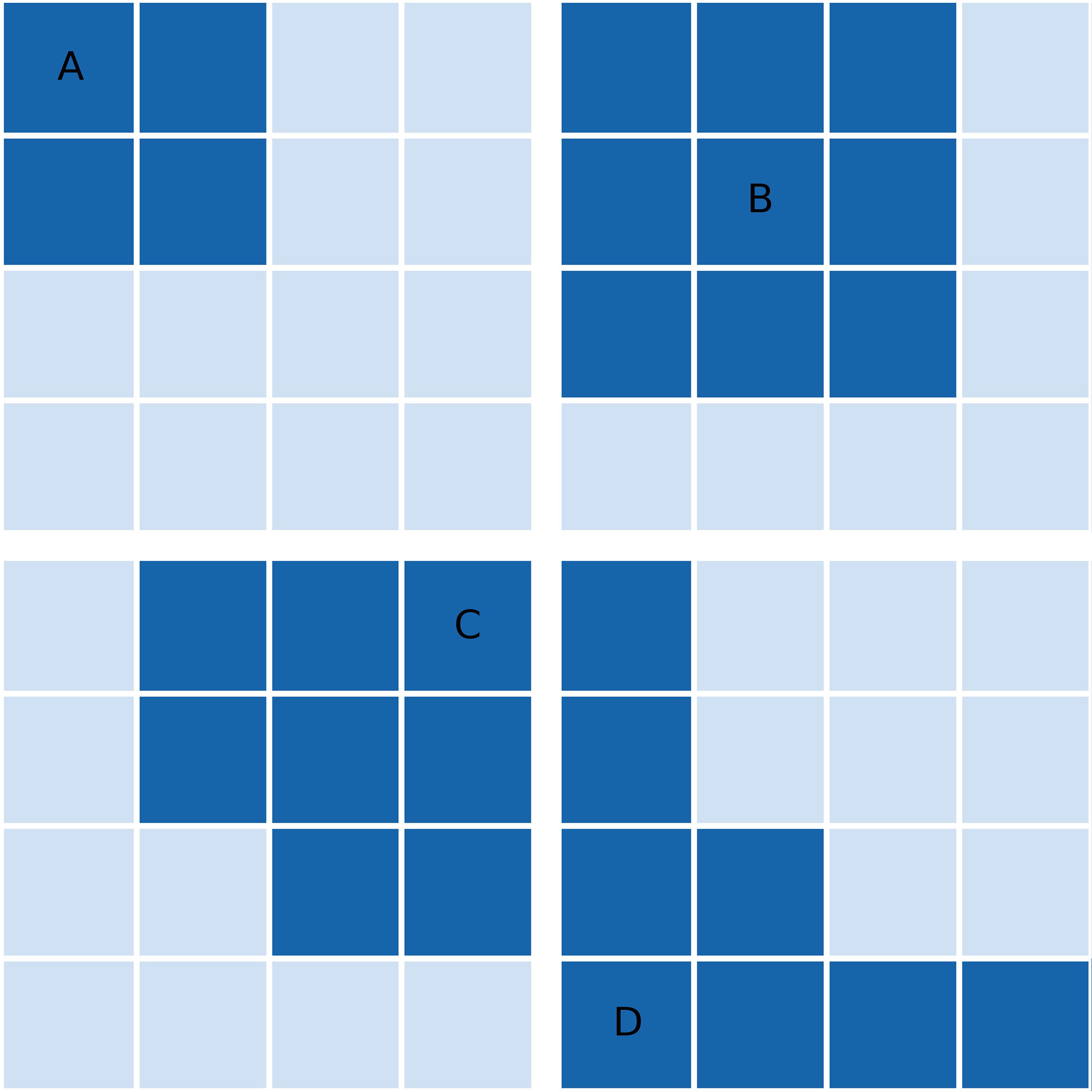
Figure 1 Demonstration of the set cover optimization problem for a set of 2D grid points (universe) and 4 subsets indicated by dark grid squares. Subsets are labelled (A–D). Of these four subsets, the greedy approximation algorithm would choose (B–D). After the reassignment step of the Modified Greedy Set Cover algorithm, (B) would be removed from the final solution as all of its points can be reassigned to (C, D).

More formally, this is often posed as follows. Suppose we have a finite set:

henceforth called the universe, and a family of sets:

such that the union of s_i is equal to U:

A set covering is any subfamily of S whose union is also equal to U (therefore S is itself a covering of U). For each subset s_i there is an associated cost c_i>0. The optimization problem is then to find a set covering X = {x₁,x₂,…,x_n} which minimizes the sum of associated costs. In the simplest case c_i may be constant for all i meaning that the objective is to minimize the total number of sets in X.

This can be further expressed as an integer linear programming problem (ILP) (Korte and Vygen, 2012). We aim to satisfy the objective function:

where

such that all elements in U are covered.

For application to observing network design, we repose the problem as:

Can we find a minimal set of observation locations which are able to fully represent (cover) all parts of a domain?

In other words, each possible observation location may be considered to represent some region of the domain. With this in mind, we would like to find a set of observations whose union represents all of the domain. This creates an additional question however: what does it mean for an observation to represent other locations? For this study, we define an observation location p₀ = (x₀,y₀,t₀) to represent another point in the domain D_i = D(x_i,y_i,t_i) to mean that the data p_i = (x_i,y_i,t_i) , can be modelled to some level of quality using only the observed data D₀ = D(x₀,y₀,t₀). An appropriate modelling scheme must then be chosen. In this paper, we use simple linear regression as our representation model and absolute linear correlations as our representation metric. Therefore, p₀ represents p_i if and only if:

where ρ is the correlation function and γ is some predefined correlation threshold. This is a similar (but inverse) concept to the effective coverage of an observation, as described by She et al. (2007) and we discuss this further in Section-2.4.4. Another way to think about this is in terms of the variance explained. Linear correlation is equal to the square root of the variance that can be explained in D_j when using a linear model in D_i . Choosing a correlation threshold of γ = 0.9 will be able to model at least 81% of the the time variance at every point in the domain using just simple linear regression. More complex methods are possible such as nonlinear models and multiple regression and we discuss these further in Section-4.

Now we must reframe this in terms of the set cover optimisation problem. We define the universe U to be the set of all n points in a given 2-dimensional domain. For computations, this domain is reshaped along a single axis. With each element of U, there is a corresponding subset s_i defined as all other points with which the data has an absolute correlation of at least γ. Therefore, the family S contains n subsets. The threshold variable γ is predefined and will affect the shape and size of each individual subset but not the number of subsets. This can be set to any value between 0 and 1, however, for small values the subsets become more irregular and noisy, so larger values are recommended.

2.2 The Modified Greedy Set Cover Algorithm

For the set cover optimization problem, there are no known algorithms which can give an exact solution in polynomial time (Korte and Vygen, 2012). For very large problems such as ours, this means that obtaining a guaranteed optimal solution is unfeasible. Instead we must obtain an optimal or near-optimal solution using an approximation algorithm that can be solved in polynomial time. There are two methods commonly used to do this: a greedy algorithm (Chvatal, 1979; Grossman and Wool, 1997; Slavik, 1997) and relaxation of the integer linear programming problem (RILP) (Grossman and Wool, 1997; Vazirani, 2001; Williamson and Shmoys, 2011). For this study we use the greedy algorithm, an iterative scheme which selects the remaining subset which covers the largest number of remaining elements in U at each iteration. It is well studied and has been shown to be the best polynomial time approximation for lower order terms (Chvatal, 1979; Grossman and Wool, 1997; Slavik, 1997; Feige, 1998; Alon et al., 2006; Grossman and Wool, 2016). As an example, in Figure 1 the greedy algorithm would select subsets in the order B, D and C.

After we obtain the greedy solution, we can improve upon it with an additional refinement step. With each observation location recommended by the greedy algorithm, there is an associated subset. As will be discussed in Section-3.1, some of these subsets are very small in areas where correlation length scales are small. In some cases, any element of one of these subsets could be reassigned to another observation where the representation metric γ is still satisfied. If all elements of one of these associated subsets can be reassigned to another point, then the corresponding location is removed from the solution. Experimentation showed that this extension to the algorithm can reduce the number of points by up to 10%. This step can also be illustrated using Figure 1. As discussed above, the greedy solution to this example yields the subsets B, D and C. However, all elements of B may be “given” to C or D, whilst still retaining a full cover of all points. Therefore, B is removed from the final solution and its elements are transferred to the subset which provides the highest correlation.

The final step is to reassign all data points with the observation that gives the largest correlation. A peculiarity of the previous two steps is that any given point may not be assigned to its best observation location. In terms of linear data reconstruction, best results will be obtained when each point is assigned to its ‘best’ observation location. We call this whole process, from greedy algorithm to final reassignment, the Modified Greedy Set Cover (MGSC), and will henceforth refer to it as the MGSC (γ) algorithm.

The algorithm may be approached from two different perspectives. Using the above method directly will give the user a set of points which guarantee a prescribed quality across the domain. The user chooses the quality and the method chooses the observing network and, importantly, the number of locations. In a realistic setting however, the observational resources available may be the determining factor and a user may want to instead specify the number of locations N. There are two ways that the MGSC method may be modified further to allow for this. The first and simplest method is to take the largest N subsets from the greedy solution. However, this means that there will be areas of the domain lacking representation. The method adopted in this paper is a further iterative scheme.

A line search type method is used (Box et al., 1969) to search through γ until the desired N is reached (or some small threshold around it). This is done by defining an initial search value γ₀ and initial search step α₀. The MGSC method is performed for these initial values and if the resulting solution does not have N observations (or within some threshold) then the search step α = α₀ is added to γ. This is repeated until the desired N is exceeded. The search step α is then iteratively halved and added to the last γ that gave a solution with less than N observations. This is done until N is reached (or within some predefined threshold). To distinguish it from the MGSC (γ) method, we call thisiterative scheme the MGSC(N) method.

It is important to note that the MGSC (γ) and MGSC (N) algorithms are close to being equivalent. Given a perfect solution using the MGSC (N), the two algorithms should give solutions that are similar. For example, suppose using MGSC (γ₀) gives a solution with N₀ points then MGSC (N₀) will inversely give a solution providing a minimum correlation of close to γ₀. In practice this is not strictly true due to the stopping conditions imposed on the line search. However, experimentation showed that for an appropriate choice of stopping parameters, these differences could be reduced to negligible levels. Consequently, throughout this paper we refer to only the MGSC algorithm where the input type is not important to the results.

2.3 Data and Experiments

In this paper we test and evaluate the MGSC algorithm. Output from the method is analysed and compared against physical quantities such as correlation length scales. We compare observing networks created using the MGSC method with two other types of network: regular and random. The random network is generated by placing N observations randomly throughout the ocean part of the domain. An ensemble of 1000 random observing networks has been generated for this purpose, and results will be presented as ensemble means and standard deviations. The regular network is created by placing observations in a regular latitude-longitude grid throughout the ocean part of the domain. This is done by extracting regular subsamples of the original data along the X and Y (lonand lat) axes. The result is that the possible values of N when generating a regular grid are a function of the original dimension sizes and the distribution of land and ocean points in the data. Therefore, N cannot be any arbitrary value in this case. When comparing to this network type, we have sometimes determined the N to be used in the MGSC and random networks from the possible values for the regular grid.

In this study we use reanalysis data based on the Coastal Ocean (CO) model configuration (O’Dea et al., 2017) to create recommendations for observing network placement. In the following sections, we look at monthly mean sea surface temperature (SST) and sea surface salinity (SSS). We have used the NWSHELF_MULTIYEAR_PHY_004_009 reanalysis product from the CMEMS database, which offers gridded data at a 7km horizontal resolution. This data covers the Northwest European Shelf, with a 3DVar system to assimilate temperature and salinity observations from profiles and at the surface. Before use, SST data is deseasoned and detrended using the statsmodels Python package (Seabold and Perktold, 2010). Observation locations and linear best fits are determined using correlations estimated from the time period 2000-2010 and data reconstruction is done using data from 2010-2020. This is to ensure that the reconstructed data are independent from the MGSC fitting procedure.

2.4 Network Scoring

2.4.1 Data Reconstruction

To help score the different network types, we use time series from observation locations to reconstruct a full dataset. As we have used absolute correlation as a representation metric, we use simple linear regression to reconstruct 10 years of temperature and salinity data. As an initial step, and for each point within a subset, a linear model must be fitted between its time series and the times series at the observation site/node. This linear model can then be used to reconstruct the time series, at the point, from the observation site alone. This fit is done using a 10-year period between 2000 and 2010. It is then used to reconstruct a time series for every location during the 10-year period 2010 to 2020. The reconstructed fields are used to obtain metrics which assess how effectively a set of locations can be used to represent the full 2-dimensional data across all length scales.

2.4.2 Correlations

Correlations form a key element of the analysis in this study. We use them both to generate observing networks using the MGSC method but also to validate them in an independent way. We use the same correlation matrix as the MGSC method to assess average and minimum levels of explained variance across the domain. Once every grid point has been assigned to the observation that best correlates with it, we may take their mean and minimum. This tells us both how well a network represents a domain on average and also identifies how it performs in its weakest areas. We also use the reconstructed dataset to assess temporal correlations independently of the fitting period. These correlations are calculated between the 10 years of reconstructed data and the actual data from that period. This will result in a 2 dimensional map of correlations, which can be averaged in order to compare network types.

2.4.3 Root Mean Square Error

Similarly, to how correlations were constructed above, we can use the reconstructed data to calculate Root Mean Square Errors (or differences). This will again give us a 2 dimensional map of RMSE, which can be averaged to obtain a single score that gives information about a networks ability to reconstruct data, and therefore represent it.

2.4.4 Effective Coverage Ratio

The Effective Coverage Ratio (ECR) describes the percentage of a gridded domain that is represented by an observing network (She et al., 2007; Fu et al., 2011). It can be thought of as the inverse of the MGSC method, deriving a score from an existing network rather than generating a network from a prescribed quality threshold. Any given grid point p₀ can be said to be ‘effectively covered’ if there is either an observation at that point or another point p₁ exists that can be used to represent it. We can then calculate the ECR taking the ratio of covered ocean points to the total number of ocean points.

3 Results

In this section we demonstrate the MGSC method and evaluate its output. We begin in Section-3.1 by viewing the direct results of the algorithm and evaluating the output. In Section-3.2, we have used the different observing networks to reconstruct 10 years of data, yielding error and correlation estimates. This allows us to score each network. Finally in Section-3.3, we present and discuss some sources of variability in the output from the MGSC algorithm.

3.1 Analysis of Algorithm

Figure 2 shows the recommended observation locations given by the MGSC(N) algorithm for SST and SSS when N = 100, 200 and 300. The shading in this figure also shows an estimate of the horizontal density of points (points per 1000km²). This has been estimated by using a radial neighbourhood averaging scheme, in which point density is calculated in successively larger radial neighbourhoods. The maximum density is taken across the resulting fields at each point. The figure shows that as N increases, the spatial structure of point density remains unchanged, with more points being added in areas of high density. This is encouraging for the MGSC algorithm as it suggests that there is an underlying structure to the output, and it isn’t randomly placed in the domain.

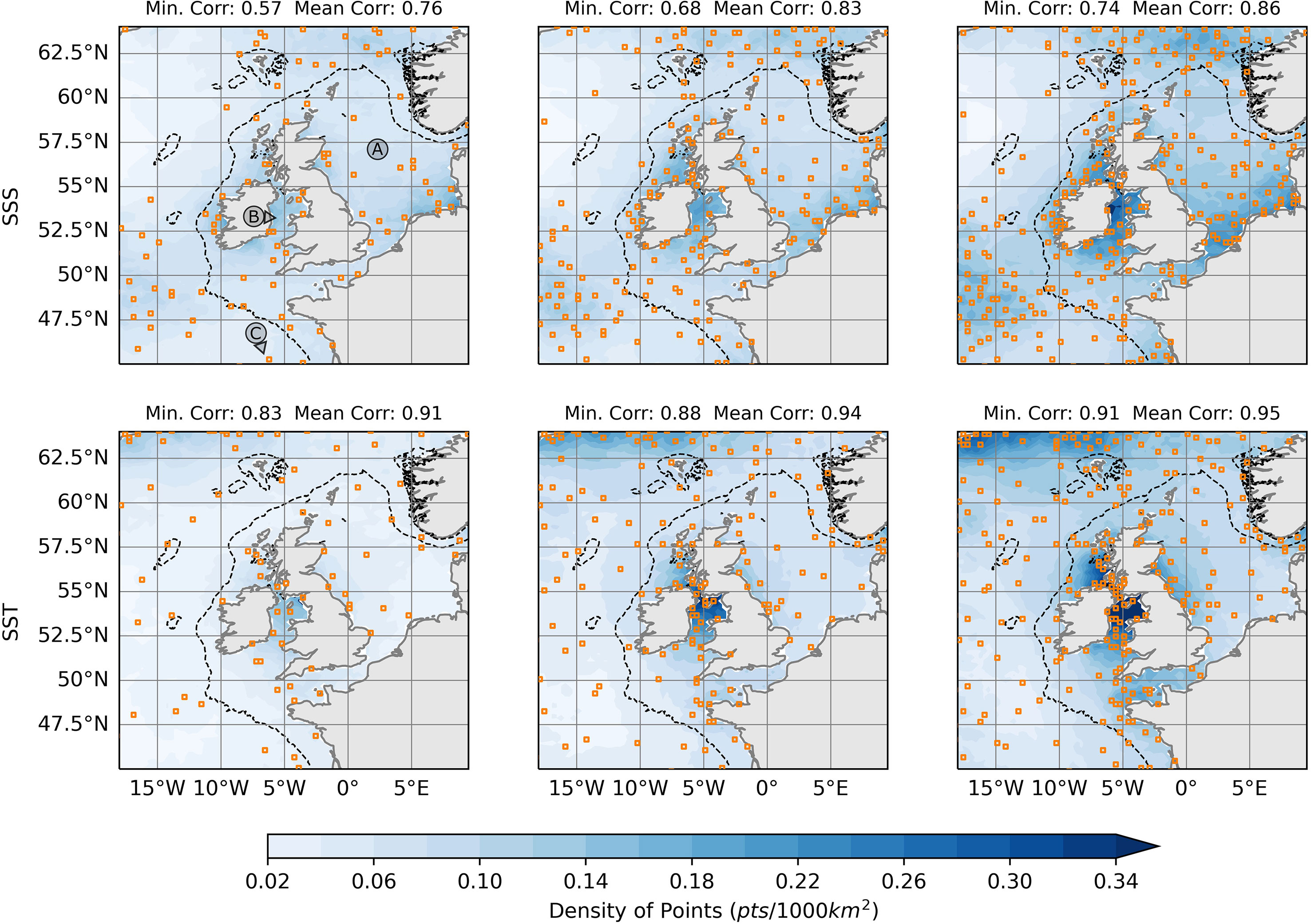
Figure 2 Suggested observation locations (orange squares) due to the Modified Greedy Set Cover algorithm for different numbers of points. Results are shown for Temperature (deseasonalized) and Salinity at 0m. The left, middle and right columns show results for 100, 200 and 300 points respectively. Blue shading shows estimates of the density of observation locations throughout the domain. Black dashed lines show the 200m bathymetric contour. In the top left panel, three geographical locations are indicated: (A) North Sea, (B) Irish Sea and (C) Bay of Biscay.

For SSS, areas of high point density are in coastal areas, especially in the Irish Sea and Southern North Sea. These are areas which are strongly influenced by river outflows and tidal flows, perhaps leading to more spatial variation at the surface. There are also two areas off shelf which have a higher density of points: in the Atlantic ocean southwest of Ireland and North of the Shetland Islands. These are areas subject to a relatively high eddy kinetic energy resulting from the tail end of Gulf Stream. We see many similar structures in SST, although there are also differences. Most notably, the density of points is greatly reduced in the southern North Sea and is increased in the Northwest of the domain. This figure also shows the minimum and mean absolute correlations achieved throughout the domain for each set of locations. We can see that as the number of points increases, so does the minimum and mean correlation for both SST and SSS. In all three cases SST obtains higher correlations than SSS, suggesting longer correlation length scales, possibly because it is strongly influenced by large scale atmospheric fluxes.

Figure 3 summarises these values for different values of N and compares them to the resulting correlations obtained when using a regular grid of observations and an ensemble of random locations. For both SSS and SST, the mean correlations are comparable across all values of N, with the regular grid being slightly better at low values and the random grids being worse across all N. However, the largest differences are seen when examining minimum correlations, which are significantly better for the MGSC method, improving upon those for the regular and random grids by 2-3 times across all N.

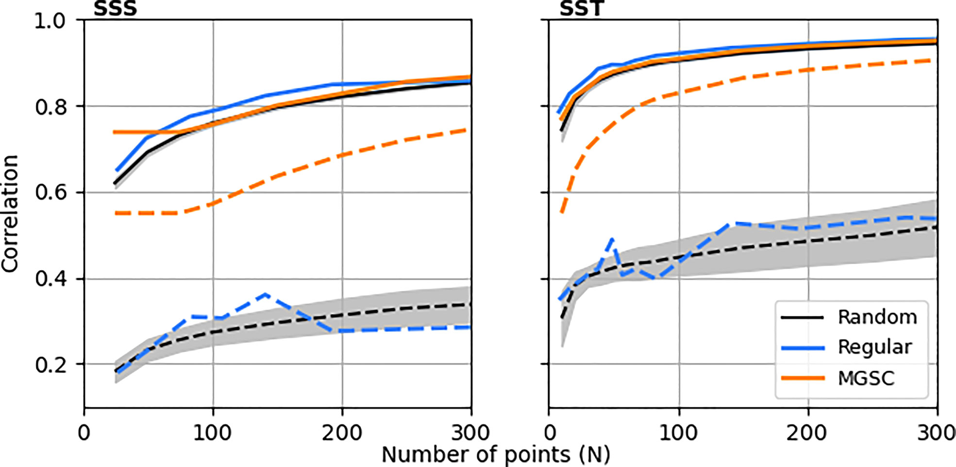
Figure 3 Mean and minimum correlations that can be achieved throughout the domain using three different observation placement methods: set cover algorithm, regular gridding and an ensemble of random placements. Solid lines show the mean correlations for each placement method and dashed lines show the minimum. For the random placements, lines show the ensemble mean and the shaded areas show 1 standard deviation either side of the mean.

This shows that the MGSC method is successfully positioning the observing network to guarantee a higher level of minimum representation without compromising the mean representation. These areas of improved representation are likely to be those with smaller correlation length scales as it is here where the MGSC algorithm places more points (discussed below). In addition, the MGSC method does not place more points than necessary in areas where length are very large. We can demonstrate this more rigorously by comparing point density estimates with correlation length scales. We estimate length scales by averaging correlations into distance bins and fitting an exponential curve of the form:

where α is a constant to be determined using a least squares fit, r is distance and p₀ is that point at which want to estimate the length scale. We use an approximate e-folding scale at each point to then estimate the local length scale by solving $\widehat{D}\left(p_0,r\right)=0.3$. Computing point densities as before, Figure 4 shows how density varies with independently calculated length scales. This comparison is shown for N = 100, 200 and 300. In all cases, there is an inverse relationship between point density and length scale, with point density decreasing as length scales increase. This confirms that the MGSC method is doing as we expected: placing more observations in areas where the dominant length scales are smaller.

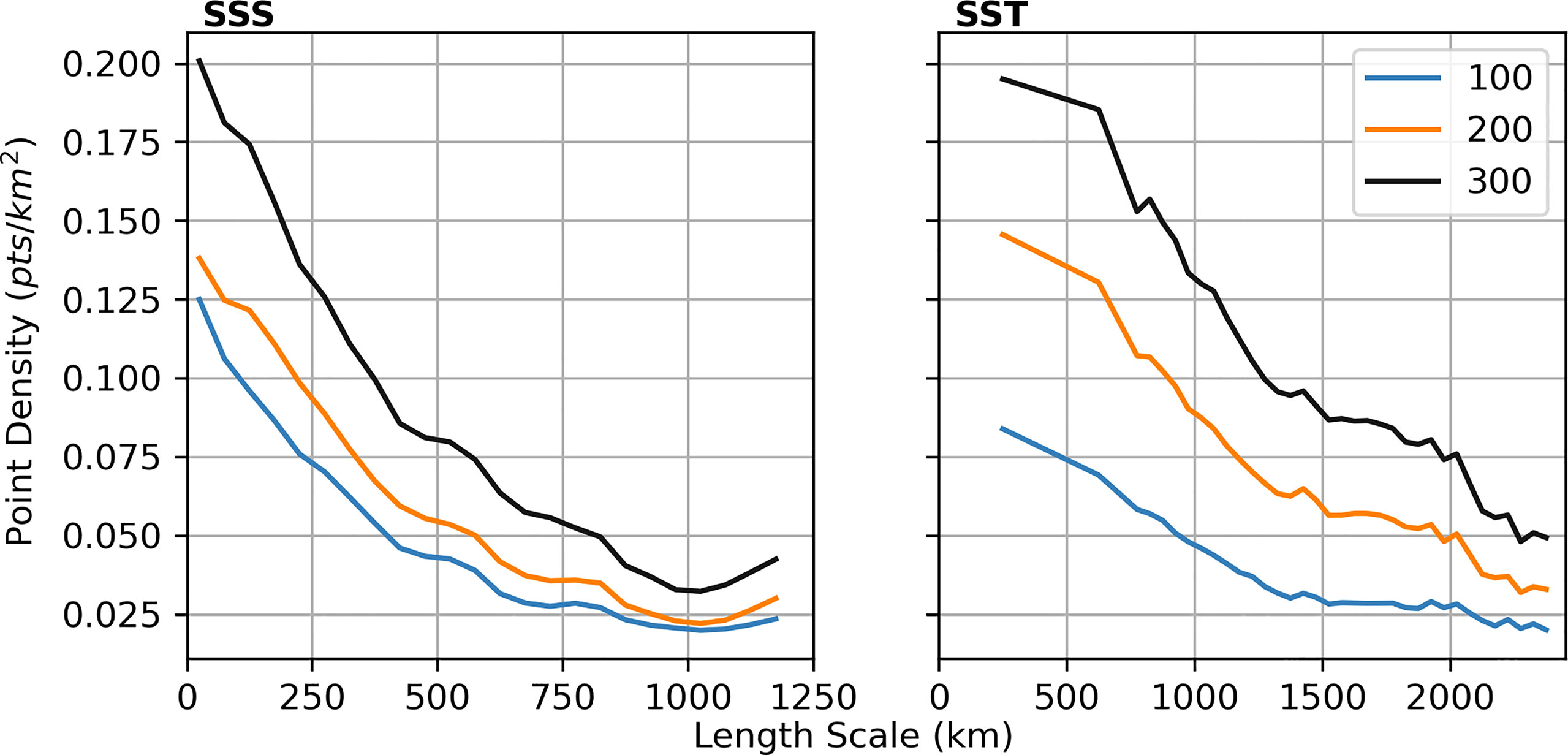
Figure 4 A comparison of length scale and observation density estimates. Observation densities are estimated from outputs of the MSC algorithm for N = 100, 200 and 300 points. The upper bounds on the x-axes are chosen to be the 97.5th percentile of the data, after which the binning process yields much noisier results due to the sparsity of data.

In Figure 5, we show an example of the correlations achieved between each point and the best associated observation location. This example is shown for SSS when again using N = 100, 200 and 300. We can see a decay in correlations away from observations, as expected. The decay rate itself is dependant upon the length scale at the observation location. This gives us a good visualization how which locations represent different parts of the domain. By comparing with Figure 2 we also get a good visual representation of the relationship between length scales and point density. In areas with higher point density, correlations decay more quickly with distance – suggesting shorter length scales. This figure also shows how the background correlations increase alongside N.

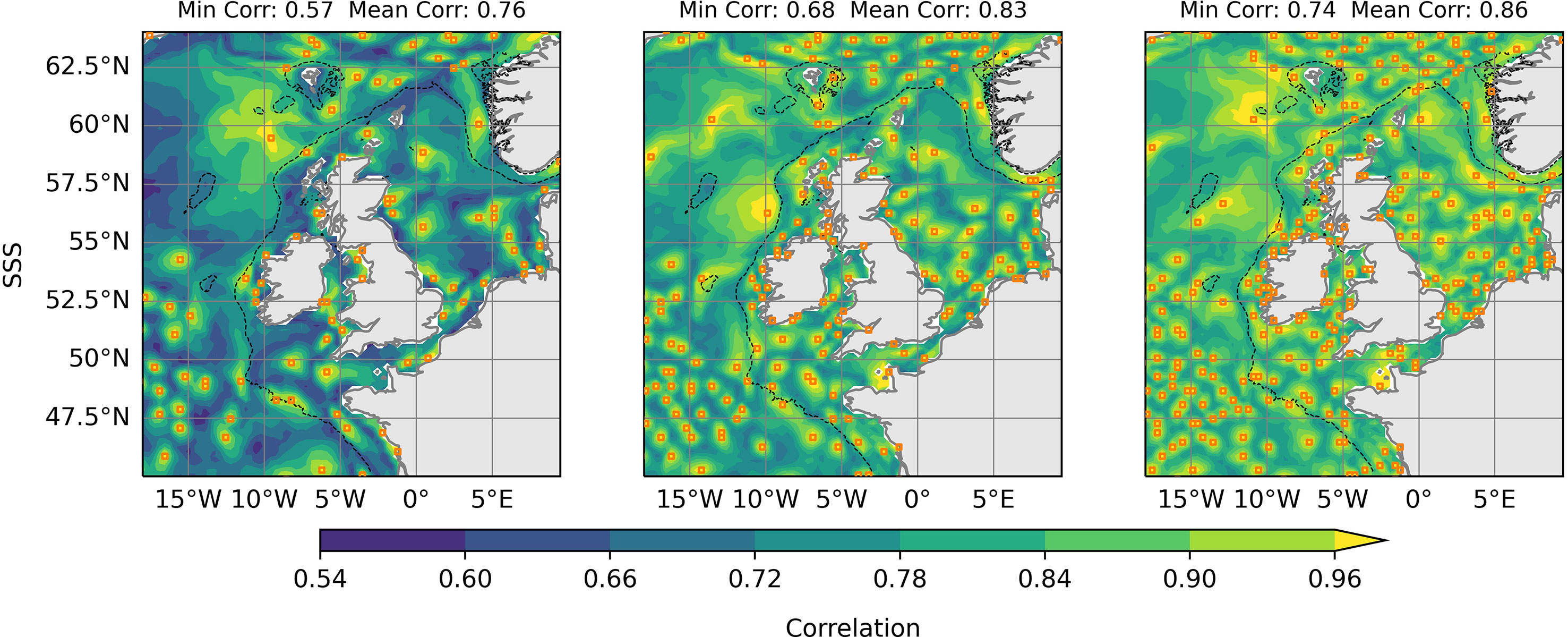
Figure 5 ‘Best’ correlations with an observation location for the Modified Greedy Set Cover algorithm. The algorithm has been run for N = 100, 200 and 300, shown from left to right respectively. Orange squares show the suggested observation locations.

Figure 6 shows a comparison of the Effective Coverage Ratio (ECR) for the three network types. This analysis was conducted by calculating the MGSC (γ) solution for a list of correlation thresholds (γ) . The equivalent or nearest network was then calculated for the regular and random cases. The ECR was then calculated using γ as its definition of coverage, as described in Section-2.4.4. Here we see that the MGSC algorithm generates a network that is able to provide a representation level of at least γ for 100% of the points in the domain. The same cannot be said for the other two network types, which fail to represent up to 15% of the domain for the regular grid and 20% of the domain for the random grids.

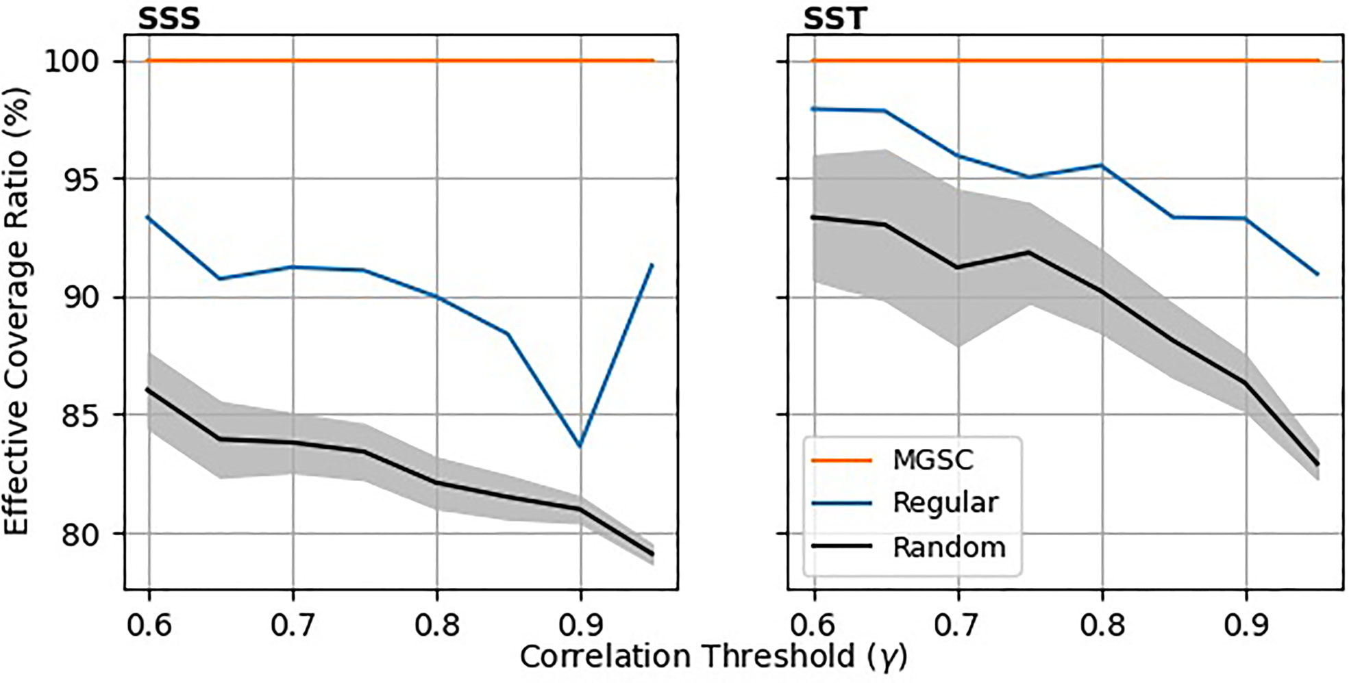
Figure 6 Effective Coverage Ratio (ECR) vs. Correlation threshold γ. The MGSC method has been used to generate a set of points for varying correlation thresholds. The corresponding regular and random grids were then generated with equivalent numbers of points. For each grid, the ECR has been calculated by using γ as the definition of coverage. For the random placements, lines show the ensemble mean and the shaded areas show 1 standard deviation either side of the mean.

3.2 Data Reconstruction Assessment

In this section, we examine and compare how effectively the different observing network placement methods are able to reconstruct a full dataset. The data reconstruction is described in Section-2.4.1.

Figure 7 shows reconstruction RMSE averaged into length scale bins. This has been done for N=198, 442 and 735, which correspond to the number of points in three regular networks of different sizes. Generally as N increases, errors decrease for all location methods, especially at smaller length scales. For the regular observation grids and random locations, errors are larger where length scales are smaller (for both SSS and SST). However, the MGSC method sees significantly smaller errors in these regions, especially for larger values of N. Figure 8 shows similar results for correlations, also averaged into length scale bins. Correlations are significantly smaller at finer length scales for both the regular and random observation placements. However, the MGSC method provides a consistent correlation level across all length scales. For smaller values of N, this means improvement at small length scales but also smaller correlations at larger length scales. This difference decreases for larger values of N.

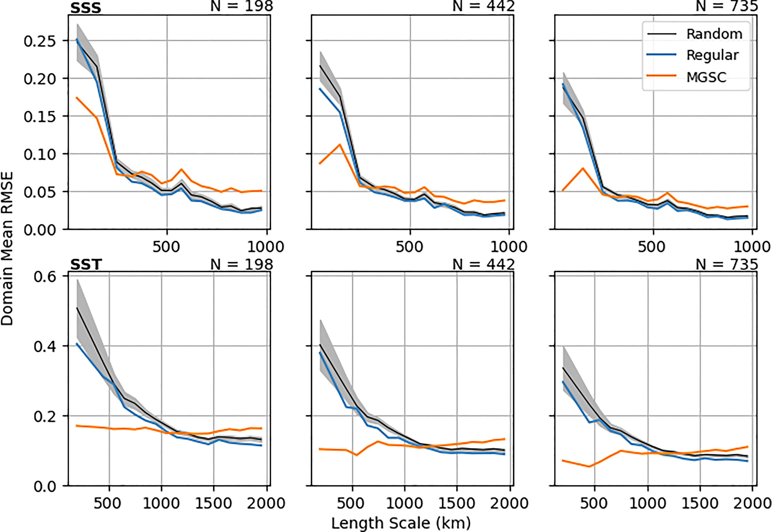
Figure 7 Area mean RMSE resulting from a 10 year data construction using simple linear regression. Means are calculated in length scale bins. Three different numbers of observations are considered (columns): N=198, 442 and 735. These values match up with the numbers of points in three different regular observation grids. For the random placements, lines show the ensemble mean and the shaded areas show 1 standard deviation either side of the mean.

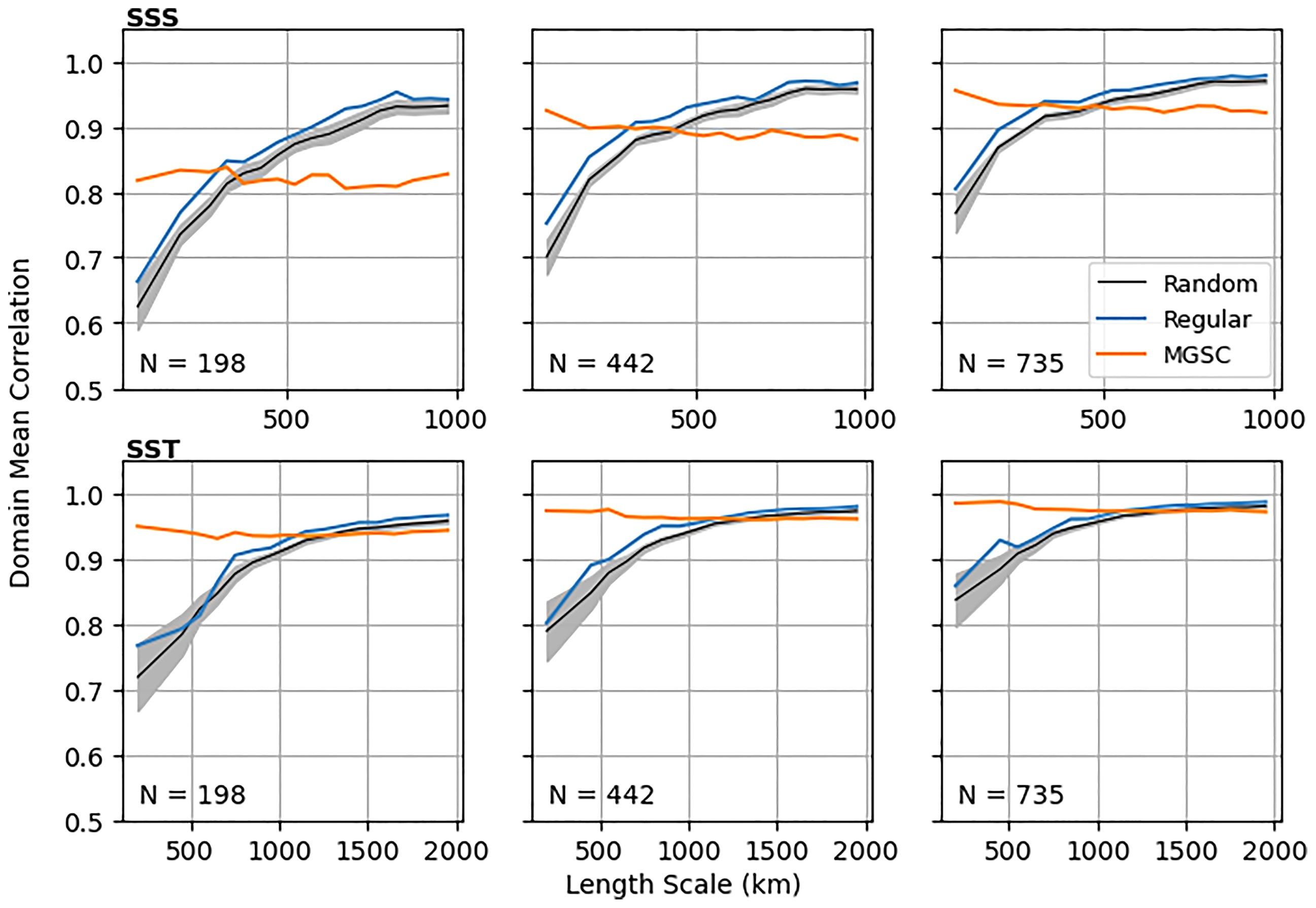
Figure 8 Area mean correlations resulting from a 10 year data construction using simple linear regression. Means are calculated in length scale bins. Three different numbers of observations are considered (columns): N=198, 442 and 735. These values match up with the numbers of points in three different regular observation grids. For the random placements, lines show the ensemble mean and the shaded areas show 1 standard deviation either side of the mean.

These results show that the MGSC method is able to provide observing network recommendations that do indeed guarantee a minimum level of representation across the domain and across all length scales. On the other hand, regular or random observation placement neglects areas of small length scales resulting in poorer representation. The improvement in these areas by the MGSC method comes at a cost however. Areas of high length scales inevitably have more observation locations when using the regular and random methods, leading to smaller errors and higher correlations for these methods. However, the MGSC method never drops below the prescribed level of quality in these areas and the difference quickly decreases as N increases.

3.3 Variability Considerations

The MGSC method will choose locations which are useful for reconstructing the time series of data that is used as an input. For example, if monthly mean data is used to estimate correlations, then the suggested observing network will be best for representing monthly mean data. Similarly, for other data frequencies such as daily means or instantaneous data. It is also important to consider how the data is filtered and variations with depth, time, horizontal resolution and domain size. We discuss these considerations further in the following sections.

In a linear context, the correlation between two random variables X and Y is related to the square root of the variance explained. As a result, if there are any frequencies in the data which dominate the variance consistently throughout the domain, then it is this that the MGSC method will attempt to capture. For example, SST is strongly influenced by a seasonal cycle in both fluxes from the atmosphere and radiative heating. This is why the temperature data was deseasonalized before being used for analysis.

We can further investigate this using an EOF (empirical orthogonal function) analysis. This is a method which can be used to decompose a 2D signal into orthogonal spatial patterns and time series. The result is a set of time series describing a consistent signal across the data (e.g. seasonality or diurnal periodicity) and associated covariance fields, which describe the 2D structure of the signal component. Figure 9 shows the largest three EOF modes for SST during the 2010-2020 period, calculated using the COAsT Python package (Polton et al., 2021). The first mode shows a domain-scale signal with an annual period that explains 93.5% of the variance in the domain. As the whole domain is moving together at this frequency, applying the MGSC method immediately to it will result in very few observation locations with very high correlations. For example, applying the method to the full SST signal shows that a minimum correlation of 0.9 may be achieved with just 5 points, as opposed to 350 when the data has had seasonality removed.

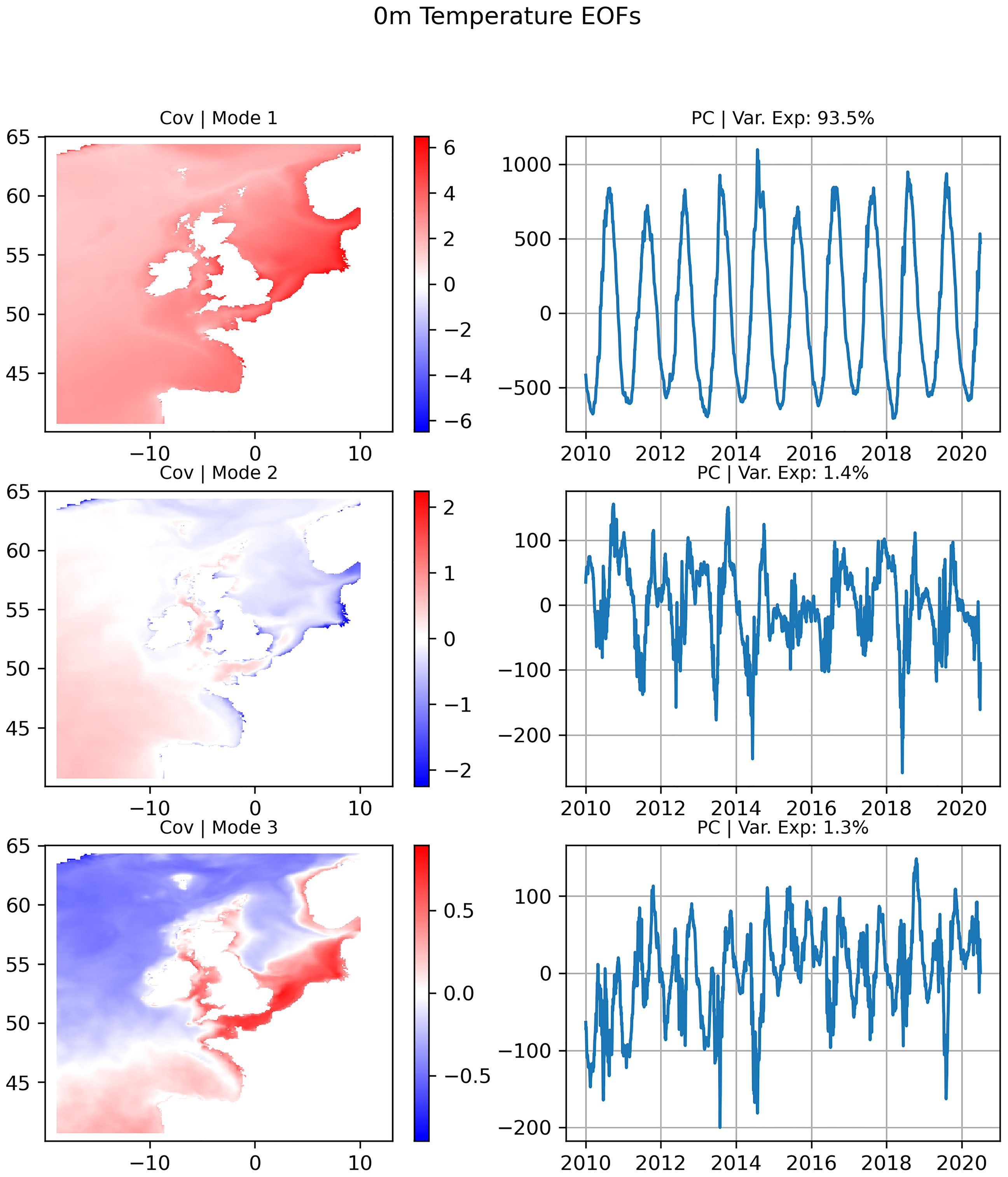
Figure 9 The 3 largest modes (top to bottom) of an EOF analysis of Sea Surface Temperature (SST). The largest mode dominates the SST signal, explaining 93.5% of the signal variance.

Of course, this is acceptable if it is the seasonal trend that the user is most interested in observing but temporal filtering is a very important aspect to consider when using the method. The MSGC method will recommended an observing network that is well suited to reconstruct the variance of the data used as input. Care must be taken when choosing how to preprocess data to ensure that it is a good representation of what you want to the reconstruct.

In this study we have presented results over a single long period of time, therefore observing network recommendations are stationary. In reality, length scales may change from month to month, season to season, over longer time periods or even with the tidal cycle. A truly automated and flexible observing system would be able to move and adapt where necessary. Below we show an example of how the MGSC algorithm can be used in an adaptive and dynamic manner, giving changing recommendations based on seasonal changes in length scales.

Figure 10 shows the difference in MGSC network placement for winter (DJF) and summer (JJA) during the 2000-2020 time period. The algorithm has been run for N = 300 points in each case presented. For SSS, 300 points is able to achieve the same level of minimum correlation of 0.76 throughout the domain and point densities are similar in most locations. There is however a notable shift of points from the southwestern North Sea in the winter to the southeastern North Sea in the summer. Differences in SST between winter and summer are more significant. A higher minimum correlation was achieved in the summer (0.92) when compared to the winter (0.89) when using 300 points. In the winter, there is a good distribution of points in most areas of the domain, however in the summer they are shifted dramatically to shallower, coastal areas. This implies finer SST length scales throughout the region during the winter.

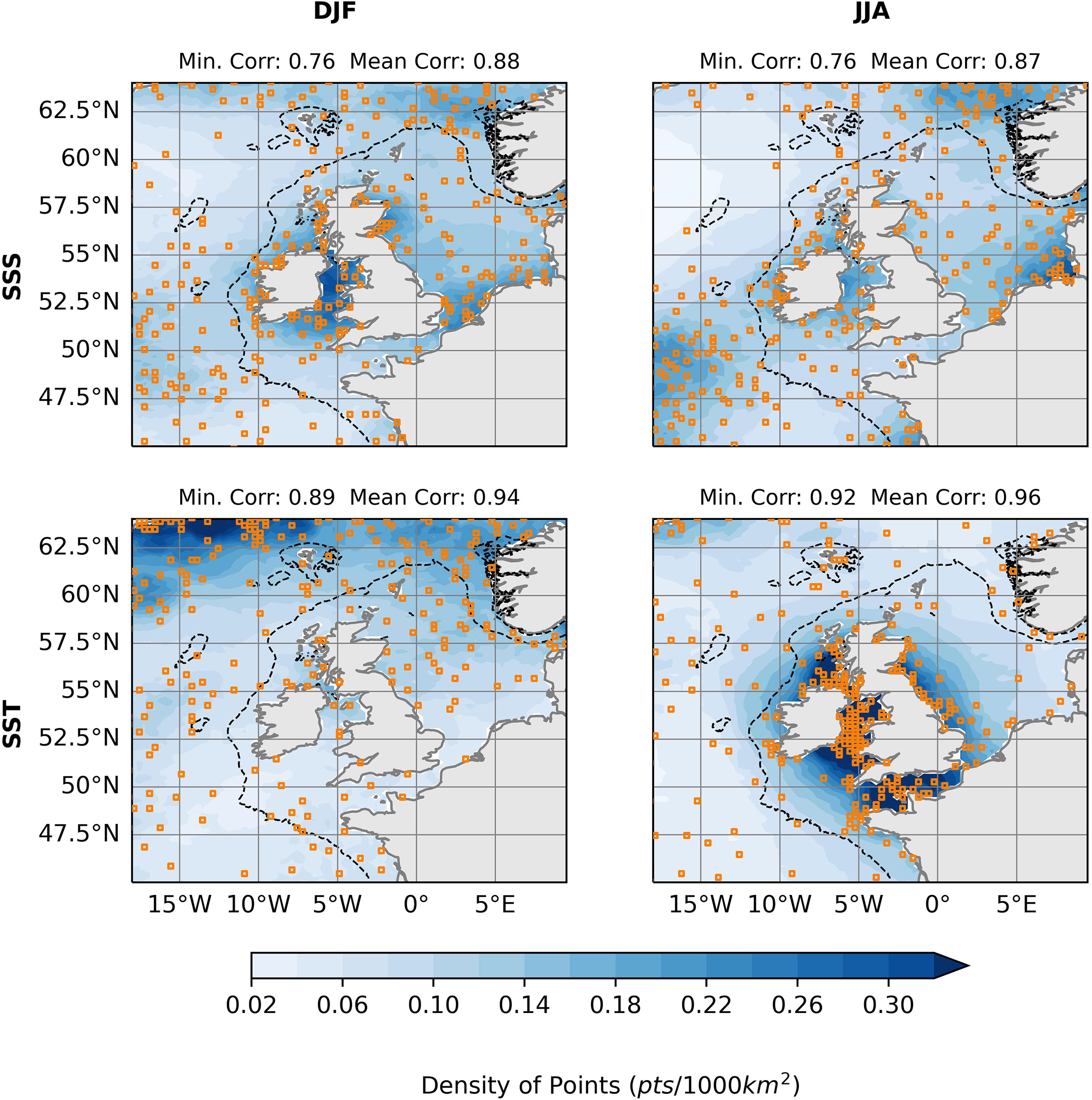
Figure 10 MGSC observing networks for N=300. Top row shows results for sea surface salinity (SSS) and bottom shows sea surface temperature (SST). Results for two seasons are shown: Winter (DJF) in the left column and summer (JJA) in the right column. Blue shading shows an estimate of horizontal point density.

As length scales can vary with depth, so will the recommendations made by the MGSC method. In this paper we have only considered results for surface variables and implicitly treated horizontal and vertical correlations as independent. Different networks may be generated for different depth levels by passing the relevant data to the algorithm. There is also no requirement for the data to lie on a specific depth level. Indeed, it could lie on any user defined surface, based on pressure, density or simply the bottom layer of the data. By generating a set of networks throughout the vertical dimension of the data, suitable decisions could be made around how to make the most of the available observations for observing the full 3-dimensional ocean. Another option is the generation of 3-dimensional correlation matrices and using these in the MGSC algorithm. This would result in a selection of volumes which would be used to represent the ocean, in place of tile shaped subsets. The problem of treating the ocean as 2-dimensional slices is common to many areas of applied oceanography, such as discussed by Levin et al. (2018). More work is required to improve the algorithm such that it does not ignore the full dimension of the true ocean and structure of observations.

The resolution of the data used to derive correlations as input to the MGSC method will affect how many locations are recommended. Coarser resolutions will not contain smaller scale features whereas finer resolutions will. The inclusion of smaller scale features may reduce length scales in some areas (depending upon how the data has been filtered), requiring additional points. Conversely, coarser resolutions will only include broader length scale features, increasing the mean length scale and decreasing the number of points required.

Figure 11 shows a comparison of the number of points required to obtain a minimum correlation of 0.75 when using data downscaled to different horizontal resolutions. Also shown is N expressed as a percentage of the total number of datapoints in each dataset of different resolution. The number of points required to maintain this correlation level decreases along with the resolution. These results offer a compromise between resource availability and the length scale which is to be resolved. If only a few new observations are available, then decisions must be made around whether it is acceptable to only represent large scale features.

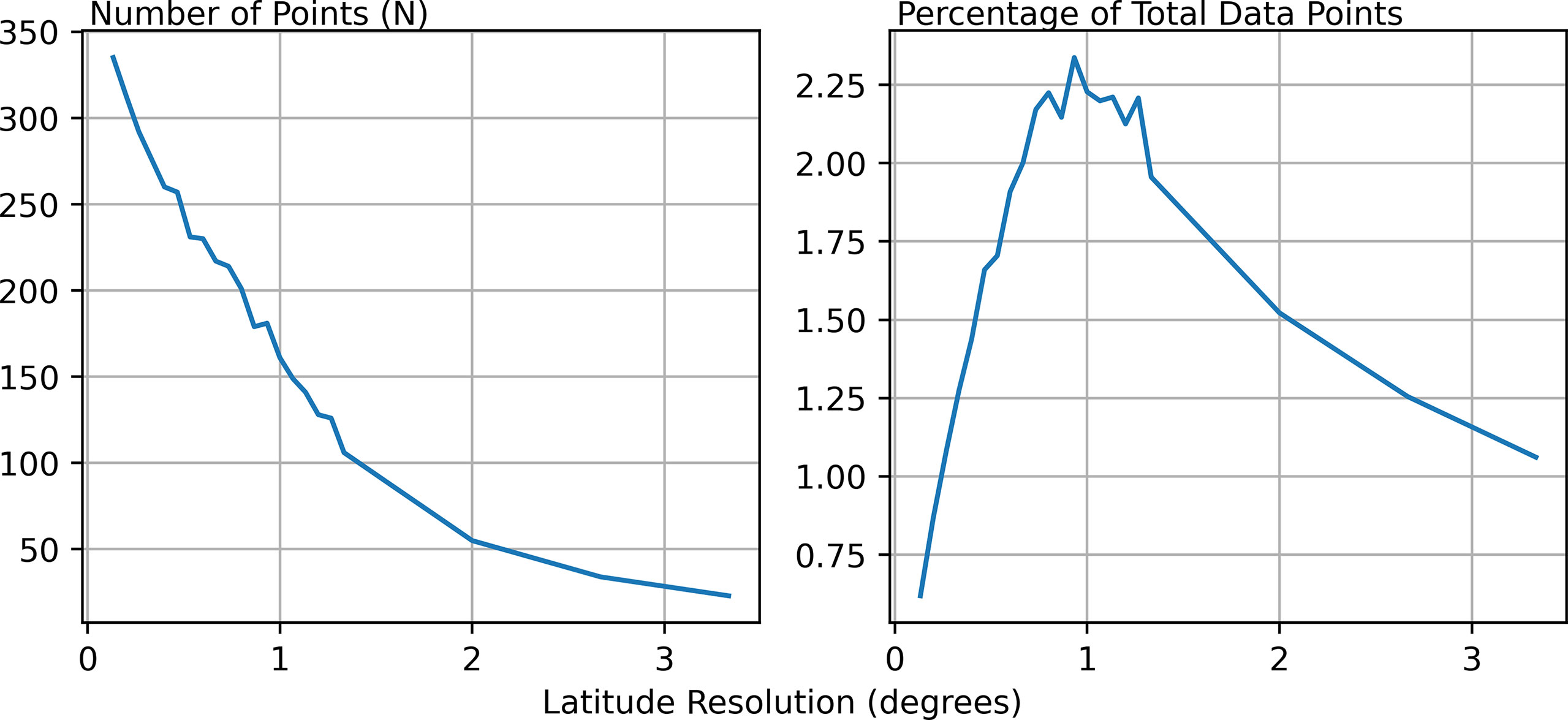
Figure 11 A comparison of the number of points required to obtain a minimum correlation of 0.75 when the data has been downscaled to different resolutions. Each plot is for Sea Surface Salinity, which is used as an example. Left: The number of points required for each downscaled latitudinal resolution. Right: The number of points required as a percentage of the total number of data points within the downscaled dataset.

4 Discussion

In this study we have introduced and demonstrated a new method for recommending how to build new observational networks – the Modified Greedy Set Cover (MGSC) algorithm. This algorithm reposed the question of where to put observations into the context of a set cover optimization problem. Our approach allows us to guarantee a minimum representation metric throughout the whole domain. In our case we used linear correlation as a measure of how well a point is represented.

The MGSC method was compared against a regular observing network and ensemble of random networks. In Figures 2–4 we presented an analysis of how well the different networks represented the whole domain. We showed that the MGSC was able to successfully prioritise higher observation densities in areas with smaller length scales. In doing so, it was able to provide a similar level of average representation whilst significantly increasing the minimum levels over the domain when compared to the regular or random observing networks. The high MGSC minimum correlation in Figure 3 indicates that by choosing MGSC as opposed to a gridded or random assignment, a monitoring network could offer an improved reconstruction of the domain using the same number of observations.

When reconstructing 10 years of data using simple linear regression, we saw similar results, which were presented in Figures 7, 8. The MGSC method provided consistent RMSE and reconstruction correlations across all length scales. When aiming to resolve all features in a spectrum of data within a domain, both the gridded and random approaches assign disproportionately high numbers of observations to regions of high length scale. These methods will resolve long length scale regions very well, but in real terms this comes at a cost to the resolution in regions of lower length scales, as seen in Figure 8. The MGSC approach will balance observations to capture features in the data across all length scales, which will generally be preferable where the aim is to measure the full range of data in the underlying population. The random or gridded approaches may be preferred in cases where only characterising large-scale variability is important and there is no requirement to know where these large-scale measurements sit in the full population of data.

This analysis described above supports our claim that the MGSC methodology offers a purely objective computer-optimised approach for placing and updating observation networks. However, implementing the MGSC output in reality may not be trivial. Our experiments (presented in Figures 9–11) showed that there is some sensitivity in the exact locations of points in an MGSC network. Exact locations may change with the data period used, the number of observations to place, depth, time frequency and data resolution. However, there is consistency in the density of points. This metric, especially with further study, may be more pragmatic for applied decision makers. Along dimensions where density may not be invariant such as depth, careful consideration must be made when designing an observing network.

In this study we have used reanalysis data to generate network recommendations and score them. This data is a combination of simulated and observed data. The full spatial realization of this data in 3 dimensions over long time periods gives us flexibility to use the MGSC algorithm for any region, any time period and any depth. It is important to acknowledge that these datasets contain errors, meaning that observation locations may not be optimal for real data. However, we don’t know the true fields (hence why we must observe) so by using accurate reanalysis data, we can still generate useful recommendations for the design of observing networks. In a completely flexible observing network, it may be possible to use an iterative process which would generate progressively better results. Each iteration would generate a reanalysis from the MGSC observations and then a new network recommendation based on that data. If the reanalysis can be improved with each subsequent iteration then so can the MGSC network. This requires further study to determine its feasibility.

We took a simple linear approach to applying the MGSC by choosing linear correlation as our representation metric. There are, however, nonlinear equivalents; using a nonlinear model (e.g. polynomial or exponential) may be more appropriate in some parts of the domain. It would be possible to extend the MGSC algorithm by looking at a collection of potential models and choosing that which fits best for each point. This would result in a set of correlation metrics (linear and nonlinear) over which the best could be chosen for each point, ensuring that the number of recommended points is reduced. The model chosen would need to be tailored to a particular observational need (e.g. marine management policy objective or scientific challenge). This extended approach would of course add to the computational resources required.

Similarly, we used simple linear regression to reconstruct a 10 year dataset from a collection of time series at the locations recommended by the MGSC method. If using a nonlinear model, then the analogue here would be to reconstruct the data using the chosen model at each location, which may vary throughout the domain. Multiple regression or ideas from data assimilation such as Optimal Interpolation or variational methods could also be used to reconstruct the data. After all, it is these methods that would be used to generate a reanalysis type dataset. An analysis of the results of this may also yield further reductions in the numbers of points required to represent the whole domain. Similarly, we have used a stationary correlation matrix, derived from using coincident time series across the domain. Extra information may be inserted into the method by using a correlation matrix derived from an analysis of lagged time series. This would be especially useful where advective effects are strong.

For this study, we have used ideas for scoring an observing network, in a similar way as you might score a model. Our work focused on the context of a simple data reconstruction, however a good observing network will serve a number of purposes. The first is (to reiterate) the ability to represent variance across all length scales and regions. Secondly, to provide a challenging validation for models. It is possible that models may appear to perform better when compared against some observing networks than others. Developing this idea of network scoring further will help ensure that these two design criteria are satisfied and will aid decision makers in the future.

Here, we have performed an in depth analysis of surface temperature and salinity. However, as remote sensing techniques improve, measuring surface values in-situ may become less important. On the other hand, oceanographic parameters cannot be acquired below the sea surface using remote sensing techniques, instead requiring in-situ using monitoring platforms such as vessels, moorings and gliders. One fundamental ocean monitoring system which could be optimised using the MGSC methodology is that of subsurface chlorophyll, oxygen and nutrient monitoring. These are routinely monitored by countries pledged to monitor and mitigate against eutrophication. Whilst coordinating in-situ monitoring systems for these mixed parameters is not a trivial task, a MGSC-based framework to coordinate and optimise these systems could become an invaluable cost-saving observation coordination tool. The tool could either distribute the available funds (consistent with the available N ) or the required accuracy requirement (consistent with a desired γ ).

In the case of eutrophication in the UK shelf seas, the environmental status is quantified through the OSPAR Commission’s Common Procedure (COMP) assessments (García-García et al., 2019). The outcomes from the COMP assessments determine whether remedial action against eutrophication is required by contracting parties of European Community legislation, in line with their obligations and commitments. A key step of these common procedure assessments is to quantify the confidence in the observations. By designing monitoring systems using the MGSC methodology, the number of monitoring platforms could theoretically be minimised whilst achieving the level of confidence required from the marine observation system.

If monitoring fails to identify developing eutrophication at an early stage (incorrectly designating an area as “non-problem” when there is a problem), there may be a range of avoidable consequences as a result of ecological damage, including financial consequences for example through impacts on tourism, fishing and carbon sequestration (Pretty et al., 2002; Jiang et al., 2018). For this reason, adequate monitoring is essential. Similarly, if monitoring fails to provide adequate evidence of good environmental status in areas where anthropogenic enrichment by nutrients does not in fact threaten the marine ecosystem, those accountable could be subjected to avoidable costs associated with emergency monitoring or unnecessary remedial work.

This work lays the foundation for a mathematical approach to generating dynamic and adaptive large scale observing networks based on reanalysis data. As autonomous observing technologies improve, this kind of approach will serve as a vital step in informing decision makers and the equipment itself. A completely flexible network may be able to shift according the seasons, the tidal cycle or climate change. If used strategically, it may be able to serve different purposes and clients on different days. These recommendations are also compatible with the large range of observation platforms available. Fixed observations could be strategically placed in areas where there is less variance in network placement. More flexible instruments could then be assigned to those areas that change periodically and quickly.

Data Availability Statement

The model data used in this paper is freely available as a part of the Copernicus CMEMS database. More information is given on the specific products used in this paper. The Python code is also openly available as a Github repository here: https://github.com/NOC-MSM/MGSC. To make this work easier to replicate, we have archived this code using Zenodo and at the time of writing the correct doi is: 10.5281/zenodo.6121062.

Author Contributions

DB lead and wrote the drafting of the article. DB undertook the algorithm and experiment design as well as data analysis and programming. DB, JH, JP, LF and JR conceived of the critical questions, contributed to manuscript drafts, provided critical feedback and approval for submission.

Funding

This work was funded by the Combining Autonomous observations and Models for Predicting and Understanding Shelf seas project (CAMPUS). Grant number: NERC NE/R006822/1.

Conflict of Interest

The authors declare that the research was conducted in the absence of any commercial or financial relationships that could be construed as a potential conflict of interest.

Publisher’s Note

All claims expressed in this article are solely those of the authors and do not necessarily represent those of their affiliated organizations, or those of the publisher, the editors and the reviewers. Any product that may be evaluated in this article, or claim that may be made by its manufacturer, is not guaranteed or endorsed by the publisher.

References

Alon N., Moshkovitz D., Safra S. (2006). Algorithmic Construction of Sets for K-Restrictions. ACM Trans. Algorithm. 2, 153–177. doi: 10.1145/1150334.1150336
Bean T., Greenwood N., Beckett R., Biermann L., Bignel P. J., Brant L. J., et al. (2017). A Review of the Tools Used for Marine Monitoring in the Uk: Combining Historic and Contemporary Methods With Modeling and Socioeconomics to Fulfill Legislative Needs and Scientific Ambitions. Front. Mar. Sci. 4. doi: 10.3389/fmars.2017.00263
Box M. J., Davies D., Swann W. H. (1969). Non-Linear Optimisation Techniques. (Edinburgh, UK: Oliver & Boyd).
Chvatal V. (1979). A Greedy Heuristic for the Set-Covering Problem. Math. Operat. Res. 4, 233–235. doi: 10.1287/moor.4.3.233
Defra (2002). Safeguarding Our Seas. A Strategy for the Conservation and Sustainable Development of Our Marine Environment (London: Department for Environment Food and Rural Affairs).
Elliott M. (2013). The 10-Tenets for Integrated, Successful and Sustainable Marine Management. Mar. pollut. Bull. 74, 1–5. doi: 10.1016/j.marpolbul.2013.08.001
Feige U. (1998). A Threshold of Ln N for Approximating Set Cover. J. ACM 45, 634–652. doi: 10.1145/285055.285059
Fu W., Hoyer J. L., She J. (2011). Assessment of the Three Dimensional Temperature and Salinity Observational Networks in the Baltic Sea and North Sea. Ocean. Sci. 7, 75–90. doi: 10.5194/os-7-75-2011
Fujii Y., Rémy E., Zuo H., Oke P., Halliwell G., Gasparin F., et al. (2019). Observing System Evaluation Based on Ocean Data Assimilation and Prediction Systems: On-Going Challenges and a Future Vision for Designing and Supporting Ocean Observational Networks. Front. Mar. Sci. 6. doi: 10.3389/fmars.2019.00417
García-García L. M., Sivyer D., Devlin M., Painting S., Collingridge K., van der Molen J. (2019). Optimizing Monitoring Programs: A Case Study Based on the Ospar Eutrophication Assessment for Uk Waters. Front. Mar. Sci. 5, 1–19. doi: 10.3389/fmars.2018.00503
Gould J., Roemmich D., Wijffels S., Freeland H., Ignaszewsky M., Jianping X., et al. (2011). Argo Profiling Floats Bring New Era of in Situ Ocean Observations. Trans. Am. Geophys. Union. 85, 185–191. doi: 10.1029/2004EO190002
Grossman T., Wool A. (1997). Computational Experience With Approximation Algorithms for the Set Covering Problem. Eur. J. Operat. Res. 101, 81–92. doi: 10.1016/S0377-2217(96)00161-0
Grossman T., Wool A. (2016). What is the Best Greedy-List Heuristic for the Weighted Set Covering Problem. Operat. Res. Lett. 44, 366–369. doi: 10.1016/j.orl.2016.03.007
Hu M.-G., Wang J.-F. (2011). A Spatial Sampling Optimization Package Using Msn Theory. Environ. Model. Soft. 26, 546–548. doi: 10.1016/j.envsoft.2010.10.006
Jiang Z., Liu S., Zhang J., Wu Y., Zhao C., Lian Z., et al. (2018). Eutrophication Indirectly Reduced Carbon Sequestration in a Tropical Seagrass Bed. Plant Soil 426, 135–152. doi: 10.1007/s11104-018-3604-y
Korte B., Vygen J. (2012). Combinatorial Optimization: Theory and Algorithms (Springer Berlin, Heidelberg: Springer).
Levin N., Kark S., Danovaro R. (2018). Adding the Third Dimension to Marine Conservation. Conserv. Lett. 11, e12408. doi: 10.1111/conl.12408
Mazloff M. R., Cornuelle B. D., Gille S. T., Verdy A. (2018). Correlation Lengths for Estimating the Large-Scale Carbon and Heat Content of the Southern Ocean. J. Geophys. Res.: Ocean. 123, 883–901. doi: 10.1002/2017JC013408
Minasny B., McBratney A. B., Walvoort D. J. (2007). The Variance Quadtree Algorithm: Use for Spatial Sampling Design. Comput. Geosci. 33, 383–392. doi: 10.1016/j.cageo.2006.08.009
Nilssen I., Odegard O., Sorensen A., Johnsen G., Moline M., Berge J. (2015). Integrated Environmental Mapping and Monitoring, a Methodological Approach to Optimise Knowledge Gathering. Mar. pollut. Bull. 96, 374–383. doi: 10.1016/j.marpolbul.2015.04.045
Nygård H., Oinonen S., Hällfors H. A., Lehtiniemi M., Rantajärvi E., Uusitalo L. (2016). Price vs. Value of Marine Monitoring. Front. Mar. Sci. 3. doi: 10.3389/fmars.2016.00205
O’Dea E., Furner R., Wakelin S., Siddorn J., While J., Sykes P., et al. (2017). The Co5 Configuration of the 7km Atlantic Margin Model: Large-Scale Biases and Sensitivity to Forcing, Physics Options and Vertical Resolution. Geosci. Model. Dev. 10, 2947–2969. doi: 10.5194/gmd-10-2947-2017
Oke P. R., Balmaseda M. A., Benkiran M., Cummings J. A., Dombrowsky E., Fujii Y., et al. (2009). Observing System Evaluations Using Godae Systems. Oceanography. 22, 144–153. doi: 10.5670/oceanog.2009.72
Oke P., Larnicol G., Fujii Y., Smith G., Lea D., Guinehut S., et al. (2015a). Assessing the Impact of Observations on Ocean Forecasts and Reanalyses: Part 1, Global Studies. J. Operat. Oceanog. 8, s49–s62. doi: 10.1080/1755876X.2015.1022067
Oke P., Larnicol G., Jones E., Kourafalou V., Sperrevik A., Carse F., et al. (2015b). Assessing the Impact of Observations on Ocean Forecasts and Reanalyses: Part 2, Regional Applications. J. Operat. Oceanog. 8, s63–s79. doi: 10.1080/1755876X.2015.1022080
Petersen W. (2014). Ferrybox Systems: State-Of-the-Art in Europe and Future Development. J. Mar. Syst. 140, 4–12. doi: 10.1016/j.jmarsys.2014.07.003
Polton J. A., Byrne D., Wise A., Holt J., Gardner T., Cazaly M., et al. (2021). British-Oceanographic-Data-Centre/Coast: V1.2.7 (V1.2.7). Zenodo. doi: 10.5281/zenodo.5638336
Pretty J. N., Mason C., Nedwell D., Hine R. (2002). A Preliminary Assessment of the Environmental Costs of the Eutrophication of Fresh Waters in England and Wales (UK: University of Essex).
Seabold S., Perktold J. (2010). “Statsmodels: Econometric and Statistical Modeling With Python,” in In 9th Python in Science Conference.
She J., Hoyer J. L., Larsen J. (2007). Assessment of Sea Surface Temperature Observation Networks in the Baltic Sea and North Sea. J. Mar. Syst. 65, 314 – 335. doi: 10.1016/j.jmarsys.2005.01.004
Slavik P. (1997). A Tight Analysis of the Greedy Algorithm for Set Cover. J. Algorithm. 25, 237–245. doi: 10.1006/jagm.1997.0887
Turrell W. R. (2018). Improving the Implementation of Marine Monitoring in the Northeast Atlantic. Mar. Pollut. Bull. 128, 527–538. doi: 10.1016/j.marpolbul.2018.01.067
Williamson D. P., Shmoys D. B. (2011). The Design of Approximation Algorithms (Cambridge, UK: Cambridge University Press).
Keywords: observations, observing networks, greedy algorithm, observing system design, set cover approach
Citation: Byrne D, Polton J, Ribeiro J, Fernand L and Holt J (2022) Designing a Large Scale Autonomous Observing Network: A Set Theory Approach. Front. Mar. Sci. 9:879003. doi: 10.3389/fmars.2022.879003
Received: 18 February 2022; Accepted: 19 May 2022;
Published: 22 June 2022.
Edited by:
Juliet Hermes, South African Environmental Observation Network (SAEON), South AfricaReviewed by:
Damianos Chatzievangelou, Spanish National Research Council (CSIC), SpainYosuke Fujii, Japan Meteorological Agency, Japan
Copyright © 2022 Byrne, Polton, Ribeiro, Fernand and Holt. This is an open-access article distributed under the terms of the Creative Commons Attribution License (CC BY). The use, distribution or reproduction in other forums is permitted, provided the original author(s) and the copyright owner(s) are credited and that the original publication in this journal is cited, in accordance with accepted academic practice. No use, distribution or reproduction is permitted which does not comply with these terms.
*Correspondence: David Byrne, dbyrne@noc.ac.uk