The Impacts of Freshwater Input and Surface Wind Velocity on the Strength and Extent of a Large High Latitude River Plume

Introduction

The northern Bering Sea and Arctic Ocean are rapidly experiencing the effects of climate change, with increasing ocean temperatures (Grebmeier, 2012; Danielson et al., 2020), loss of sea ice (Stabeno et al., 2019), increasing river flow (Feng et al., 2021), and mobilization of long buried carbon from permafrost into aquatic systems (e.g., Rawlins et al., 2019). The relatively shallow bathymetry and large freshwater input make the Arctic the freshest of the major ocean basins, with riverine input of freshwater and terrestrial material imprinting on the Arctic Ocean physics and biogeochemistry throughout the basin. A significant amount of organic matter is transported by these rivers into the ocean, including particulate organic carbon (POC; McClelland et al., 2016) which can be deposited into the shallow coastal seas, and dissolved organic carbon (DOC), which can be transported further from the coast and into deeper marine waters (Fichot et al., 2013). Historically, a large amount of ocean water (∼0.8 Sv; 1 Sv = 1 km³ s^–1) (Roach et al., 1995) enters the Arctic through the Bering Strait, where the mean flow from the northern Bering Sea brings fresher continental runoff into the Arctic. In the last three decades there has been an increase of ∼20% in the northward transport of water through the Bering Strait, with flow increasing to 1.0 ± 0.05 Sv (Woodgate, 2018).

The input of freshwater and material along the Alaskan coast has the potential to be transported through the coastal current system into the Arctic, likely impacting the regional and global freshwater budgets and carbon cycles. Key processes related to POC and DOC transformations such as flocculation and settling occur in regions with strong salinity gradients within river plumes. The lack of knowledge of the spatial and temporal variability of the coastal currents in the northern Bering Sea at the outflow of the Yukon River make generalizations of the transport of riverine water and material from the Northern Bering Sea into the Arctic difficult. The coastal dynamics where the Yukon plume enters and mixes with marine water in the shallow and broad shelf are not thoroughly characterized even though the contribution to Arctic biogeochemical processes is likely large.

The Yukon River is the 5th largest river in North America, and the longest free-flowing river in the world (Yukon River Inter-Tribal Watershed Council, 2021). It is the 5th largest of the Arctic Great Rivers (Shiklomanov et al., 2021) by annual volume with a median discharge of 207 km³ year^–1 from 1977 to 2019 (Clark and Mannino, 2021). Like other polar rivers, it is highly seasonal with discharge peaking in spring upon ice breakup, sustaining throughout the ice-free season with substantial interannual variability, and declining substantially from the fall into the winter. The Yukon has the highest sediment yield per unit watershed area for the six largest Arctic rivers, with 67 Mg km^–2 year^–1 of total sediment entering the ocean on average (Piliouras and Rowland, 2020). In addition, DOC yield per watershed area is the third largest among the six largest Arctic rivers at 625 mg C m^–2 year^–1 and 1.5 Tg C year^–1 of DOC is transported to the ocean from the Yukon basin on average (Holmes et al., 2012). With the mean northward current and shallow coastal bathymetry, a substantial portion of Yukon derived DOC may be transported through the Bering Strait contributing to the Arctic carbon budget. The time and space scales of transport of the riverine water along the coast likely exhibit substantial control on the quantity and composition of the material that flows through the Bering Strait into the Arctic as various biogeochemical reactions occur in and outside of the plume.

River plumes are highly complex hydrographic features in the coastal ocean where freshwater enters, stratifies, and mixes with oceanic water. River plume characterization exists along a continuum (Horner-Devine et al., 2015), and sampling and mathematical methods used to quantify the distribution of freshwater in the coast are varied and complex. The amount of freshwater and the geomorphology of the river channel adjacent to the coast are the first order controls; high discharge and a narrow channel will lead to a large plume and a prototypical river plume structure, while a large estuary or deltaic environment can lead to substantially different plume dynamics (Horner-Devine et al., 2015). External forcing such as tidal currents and wind stress can also affect how river plumes mix, evolve, and disperse in space and time in the ocean (e.g., Fong and Geyer, 2001; Pritchard and Huntley, 2006; Banas et al., 2009; Horner-Devine et al., 2015). The interplay of these external factors and the volume and timing of riverine discharge into the ocean will largely control the distribution of the plume from the outflow into deeper marine waters.

The main physical drivers of plume mixing dynamics shift as distance from the river mouth increases within large river plumes and other density stratified systems (Fong and Geyer, 2001; Hetland, 2005). Specific regions where mixing dynamics shift have been defined as the near-field, mid-field, and far-field areas, although the boundaries between these regions are rarely strongly delineated (Horner-Devine et al., 2015). In the near field just outside of the mouth, inertial flow from the momentum of river discharge dominates, and stratification is minimal as the water column remains vertically uniform and relatively fresh (Horner-Devine et al., 2015). Beyond this, stratification sets in as the bathymetry begins to slope away and buoyancy driven flow due to density stratification combined with the Coriolis force and centripetal acceleration can develop a large “bulge” offshore (Yankovsky and Chapman, 1997; Horner-Devine et al., 2015). Further offshore in the far-field of the plume, the Coriolis force and wind driven mixing exert a stronger influence on plume dispersion (Hetland, 2005; Horner-Devine et al., 2015). The balance between vertical shear, stratification, and inertial flow is critical in governing the overall structure of the plume as it evolves in space and time.

Wind stress is an important external forcing factor that can drive currents in the coastal ocean and affect how mixing occurs within a river plume (Hetland, 2005). The balance of wind-driven and buoyancy-driven flow will have a strong influence over how the plume is distributed in time and space for a given system beyond the frontal region (Whitney and Garvine, 2005). Wind regimes in the coast are generally categorized as “upwelling” or “downwelling” which refers to the wind’s imparted effect on the coastal ocean currents either “pulling” water up from depth to the surface with a mean flow offshore, or “pushing” water down from the surface to depth with a mean flow onshore (Fong and Geyer, 2001). Downwelling winds tend to enhance the mean along shore current, increasing surface velocity within a plume while narrowing the horizontal extent of the plume and deepening the depth of the pycnocline (Fong and Geyer, 2001). Upwelling winds tend to have the opposite effect, narrowing the vertical extent of the plume while broadening the horizontal extent offshore due to the competing wind velocity and mean current flow and the Ekman transport of water offshore. The scales of mixing and how the plume currents and density respond to surface wind stress will likely impact coastal riverine material retention, distribution, and particulate deposition in the near shore region.

The hydrodynamic and circulation features of the lower Yukon River, delta, plume, Norton Sound and adjacent Bering Sea are understood only from a broad large-scale perspective with limited historical observational studies (e.g., Dean et al., 1989). In this study, a high-resolution numerical ocean model was constructed to characterize and predict fine-scale ocean hydrodynamics in the Yukon River plume, Norton Sound, and the coastal northern Bering Sea (hereinafter YukonFVCOM). The model was implemented over 7 years and used to estimate the hydrographic patterns at the outflow of the Yukon River. In addition, specific strong wind events were identified in each year to better estimate the effects of wind forcing on the plume structure and distribution. This allows a detailed characterization of the driving forces that govern the river plume structure in space and time.

Materials and Methods

The Finite Volume Community Ocean Model Description

The Finite Volume Community Ocean Model version 4.3 (FVCOM) is an unstructured grid ocean model designed to simulate ocean physics in locations with complex geography and bathymetry (Chen et al., 2013). It is ideally suited for use in coastal ecosystems such as the Yukon River outflow where flexible model grid geometry allows for including the river delta in the model domain and shallow coastal bathymetry can be well represented. The FVCOM model has been implemented in the Arctic to simulate coastal currents and sea ice on multiple time and space scales and shows good agreement with observations in the region (Chen et al., 2016). FVCOM calculates velocity, momentum, density (ρ), temperature (T), and salinity (S) (among other hydrographic variables) in the water column and offers a prediction of the physical conditions in the coastal ocean. The YukonFVCOM grid is made of 756,241 elements connecting at 435,240 nodes spanning from ~200 km upstream of the coast at Pilot Station, AK, to south of the Yukon delta northward to west of Nome, AK encompassing nearly all of Norton Sound and the Yukon delta (Figure 1). Grid spatial resolution stretches from ∼100 m in shallow coastal and deltaic areas to ∼2.5 km offshore (Supplementary Figure 1) with 10 vertical layers each comprising 10% of the water column at any given location. T, S, ρ, and sea surface height (η) are calculated at the nodes of the triangular mesh, and u and v current velocity vector components are calculated at the element centers. While intertidal wetting and drying is an important feature of FVCOM, we did not implement the scheme here as the focus of the study was in the ocean rather than intertidal regions.

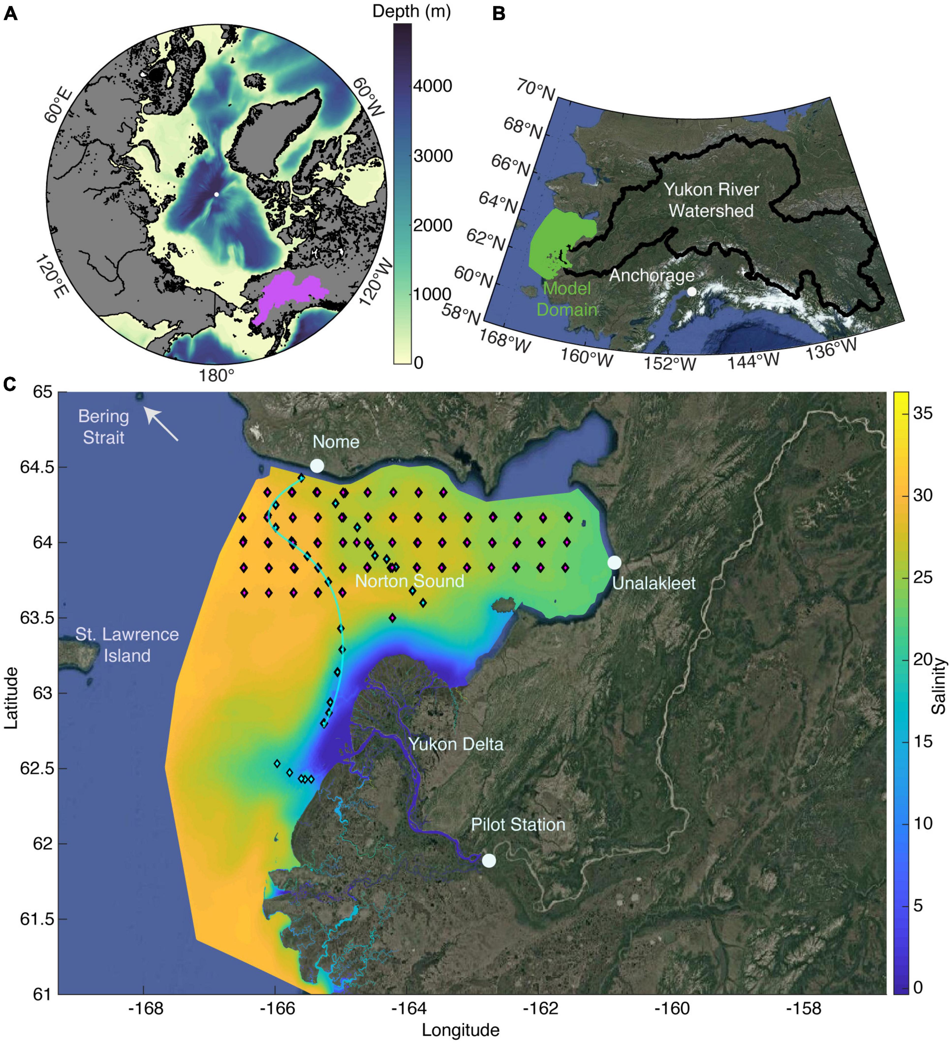
Figure 1. (A) The Arctic Ocean showing the Yukon River watershed in purple; (B) Alaska and western Canada showing the Yukon watershed with the extent of the Yukon River FVCOM hydrodynamic model domain (YukonFVCOM); (C) the YukonFVCOM model domain with Alaska Department of Fish and Game (ADF&G) fishery survey stations as red markers and the stations sampled under the NASA RSWQ project in 2019 as cyan markers. The color contours are the average surface salinity predicted by the model for 2019. Panel (A) was created using the m_map toolbox (Pawlowicz, 2020) and the images in panels (B,C) were created using the MATLAB function Plot_Google_Map.m (Bar-Yehuda, 2021).

To build the model grid, United States Geological Survey (USGS) HUC-8 watershed boundaries and Norton Sound coastline along with the USGS NED-8 Alaska digital elevation model were loaded into the Aquaveo^® SMS meshing software to construct the unstructured triangular mesh based on the bathymetry. The model was built for the period of April 1 to September 30 for 7 years spanning various hydrological patterns (Table 1). The initial condition was set for every year using the output from September 30 of 2004 after three sequential simulations to equilibrate the salinity field. This was done for consistency upon initialization and with the assumption that by the time model analysis was initiated in May of each year, the ocean temperature would have equilibrated with the atmosphere and any residual salinity would have dissipated. The spring freshet generally occurs over May and early June (Table 1). Two anomalous years with regards to ice and river discharge were 2019 and 2005, respectively. In 2019, sea ice was virtually non-existent in Norton Sound (National Snow and Ice Data Index¹), and the largest discharge on record occurred in 2005 with a very early ice break-up and spring freshet (Table 1).

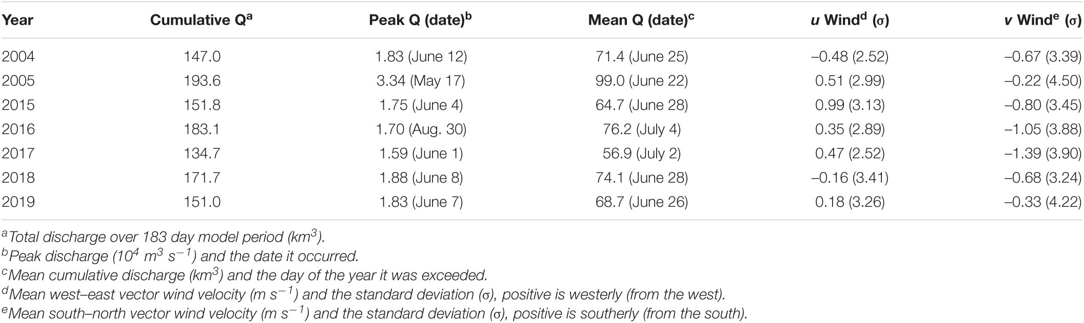
Table 1. Annual discharge (Q) and wind velocity vector components of each model year used in the FVCOM hydrodynamic model analysis.

The model was constructed and run on the NASA Center for Climate Simulation supercomputer Discover at NASA Goddard Space Flight Center. Forty compute nodes utilizing 28 out of 40 cores on each node were used for each simulation year taking 10–12 wall-clock hours to run with the 1,120 processes. The model internal time step was 6 s and the external time step was 2 s. Model output is in NetCDF format at hourly intervals and the output files were averaged as necessary using the NetCDF Operators (NCO) toolbox to generate monthly average composites².

Yukon River and Norton Sound Model Domain

The Yukon River is the 5th largest river routinely sampled as part of the Arctic Great Rivers Observatory (ArcticGRO) with daily gauge records going back to 1977. Under ArcticGRO, high quality biogeochemical observational data (Holmes et al., 2021) are collected at Pilot Station, AK, United States (61.9344°N, –162.881°W) (Figure 1) at USGS gauge station 15565447 making this an optimal Arctic River system for modeling hydrodynamic-biogeochemical interactions. Pilot Station is located ∼200 km upstream from the outflow of the delta region that drains into the shallow Norton Sound, with ∼95% of the 824,400 km² watershed located above the gauge station (Figure 1B). The watershed is underlain with 58% discontinuous permafrost (Holmes et al., 2012), and like other Arctic systems the discharge is highly seasonal with a peak occurring in late spring after ice break up and secondarily in later in the summer due to processes in the interior of Alaska such as rain events or melting snow and glaciers (Dornblaser and Striegl, 2009).

Tides, Meteorology, Open Boundary, and River Forcing

Four key external forcing factors are required to set up the FVCOM model. First, the open boundary surface elevation that drives the tidal elevation and tidal velocity in the coast was built using the TPXO software (Egbert and Erofeeva, 2002). This software is commonly used to predict tidal elevation in space and time throughout the globe. The model boundary node coordinates (n = 389) and hourly time intervals for each year were input to the software to predict the tidal elevation at each boundary node for the model time period.

The surface meteorology was built for each year using daily predictions of weather conditions from the North American Regional Reanalysis (NARR; Mesinger et al., 2006). Wind vector velocity (m s^–1), air temperature (°C), relative humidity (%), surface pressure (Pa), and net short wave and long wave radiation (W m^–2) were used as the weather forcing of YukonFVCOM. Daily average wind velocity is used to predict wind-stress on the surface of the ocean model and wind roses for each year can be found in supporting information (Supplementary Figure 2). Relative humidity, air temperature, surface pressure, and radiation are used in the COARE2.6 algorithm (Fairall et al., 2003) to calculate the heat flux between the ocean and the atmosphere at each time step. To apply the 32 km NARR data to the high-resolution grid, all NARR grid points over the model domain were extracted for each variable. Next, the gridded weather data were interpolated onto each of the model triangular cells using a nearest-neighbor interpolation. Norton Sound is covered with sea ice in the winter and early spring, but dynamically modeled sea ice was excluded from this effort to reduce complexity, therefore model analysis (unless otherwise specified) began on May 1 after spin-up over the month of April and early May to allow the model to equilibrate.

The open boundary water column T and S fields were constructed using the World Ocean Atlas 2018 (WOA18) T and S climatologies for each decade (Locarnini et al., 2018; Zweng et al., 2018). Monthly climatologies of each variable were downloaded and the closest points of the global WOA18 1° grid to the model boundary nodes were identified. For each month, WOA18 T and S were interpolated in three-dimensional space (longitude, latitude, and depth) onto the curved model boundary using the MATLAB^® function griddatan.m. FVCOM linearly interpolates between input time points to match the time step within the model from the monthly climatological values.

Last, daily mean river discharge and water temperature at Pilot Station, AK were downloaded from the USGS³ and implemented directly for each day in the model time frame. Figure 2 shows the entire gauge record from 1977 to 1996 and 2001 to 2019. The daily discharge values were evenly split over the nine model nodes that makeup the landward model boundary which begins at Pilot Station and flow was evenly applied vertically in the water column. Substantial variability exists in the model years in timing and magnitude of the freshet, in addition to total discharge, offering a wide range of riverine conditions to assess how freshwater input can affect coastal ocean hydrography. Table 1 provides a summary of freshwater input parameters and average wind vector velocities for each model period.

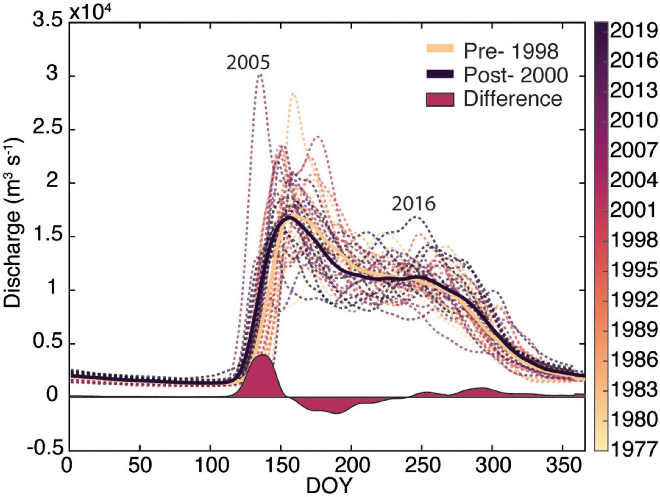
Figure 2. United States Geological Survey (USGS) daily mean river discharge at Pilot Station, AK, United States for the period from 1977 to 2019. The difference is between the mean pre-1998 and post-2000 discharge.

Model-Data Comparisons for Validation

Three sources of in-situ data were used to assess the predictability of the YukonFVCOM T and S fields in time and space. The Alaska Department of Fish and Game (ADF&G) conducted surveys in 2017, 2018, and 2019 of fish stocks in Norton Sound where T and S vertical profiles were collected across Norton Sound during the summer (Figure 1C). In addition, 40 T and S vertical profiles were collected under the National Aeronautics and Space Administration (NASA) Remote Sensing of Water Quality (RSWQ2019) project #80NSSC18K0492 (PI Hernes, UC Davis) in late May and June of 2019 in the Yukon River delta and Norton Sound. All ADF&G and RSWQ2019 sampling stations used for the model skill assessment are shown in Figure 1C. The National Oceanographic and Atmospheric Administration Tides and Currents stations at Nome, AK and Unalakleet, AK were used to assess the models ability to predict η. The station at Nome is very close to the model boundary and therefore suffers some boundary effects, while the station at Unalakleet is deep in the model interior in Norton Sound and is therefore the best assessment of the predictive capacity of YukonFVCOM for η. The closest model nodes in space and time were matched with the CTD casts and the tide gauge stations for a statistical comparison using the correlation coefficient (r), Nash-Sutcliffe model efficiency (MEF), and RMSD as the primary metrics (Stow et al., 2009).

Sea surface temperature (SST) was validated for each year using satellite data acquired from the NASA Level 2 Ocean Color Browser (Nasa Goddard Space Flight Center, Ocean Ecology Laboratory, Ocean Biology Processing Group, 2020). Images with 100% spatial coverage over the model domain were downloaded at Level-2 daily for the 4 and 11μm temperature products from MODIS-Aqua (all years) and 11 μm VIIRS-Suomi-NPP (2015–2019) (JPL/OBPG/RSMAS, 2020). Monthly mean composites were constructed from each set of individual daily images by finding all images within a month and averaging through time. Each node in the model was assigned the closest satellite pixel in the image and the set of images were “stacked” in an array (number of model nodes × number of images) for each month. Finally, the monthly mean was taken excluding the points within each image that were masked to build a nearly complete monthly composite of SST over the ocean. Because of the large amount of satellite data and model output to compare (435,240 points × 5 months × 7 years), a target diagram approach was used to easily display the model-data comparison while assessing the predictive capacity of the model (Jolliff et al., 2009). The unbiased root mean square deviation (uRMSD) was scaled by the sign of the difference between modeled and observed standard deviation, so points on the left (right) of the origin indicate less (more) spatial variability in the modeled prediction vs. the observed. Bias is a measure of the direction and magnitude of the modeled SST relative to the observed with a negative bias indicating the model values are less than observations for that month. An example monthly satellite - YukonFVCOM SST comparison from August of 2019 can be found in Supplementary Figure 3. The same sign convention holds for the target diagram comparisons of the CTD casts.

Model Output Analysis

Monthly averaged model results were compiled for each year by averaging each NetCDF output file along the time dimension. A model transect was extracted along the blue-marked cruise track in Figure 1C, corresponding to the RSWQ2019 cruise from Nome toward the south Mouth of the Yukon River delta. This was done by finding the closest element centered points along the track evenly spaced at 200 m. To get element-centered T, S, and ρ, the average of the three nodes of each element were calculated. Much of the analysis related to plume dynamics and extent was reduced to this transect for simplicity, while maintaining a gradient from freshwater and across Norton Sound.

Multiple metrics related to the velocity field, density, and buoyancy were calculated to relate river forcing, wind velocity and coastal currents and plume distribution in the coastal ocean. First, vertical shear was calculated using Eq. 1 where u and v are the west–east and south–north (positive is north and east) current velocity vector components, z is the depth, and dU dz^–1 is the vertical shear. Equation 2 represents the formulation used to calculate the Brunt-Vaisala frequency, N² (s^–2) where g is the acceleration due to gravity (9.8 m s^–2), and ρ is the density calculated by the equation of state from the predicted T and S. The effect of pressure on density was assumed to be negligible because of the shallow depth of our study domain. All vertical gradients were calculated at model intra-sigma levels (n = 9). N² is a measure of the stratification stability of a water column with a greater N² indicating stronger stratification and water column stability.

Semi-variograms for u and v current velocity and salinity were calculated using the MATLAB file exchange toolboxes variogram and variogramfit (Schwanghart, 2020a,b). Variograms are a measure of the spatial autocorrelation of a dataset and are commonly used in geostatistical modeling to predict intermediate values in a sampled data set (Matheron, 1963). Here, the variograms were used to quantify the spatial variance for each year to assess the interannual similarity (or difference) in the spatial patterns of the salinity and velocity fields. Semi-variogram analysis was conducted by finding all pixels in the model where the salinity was greater than 2.0 to avoid issues relating to calculations occurring by relating points that are close in spatial proximity but are separated by land in portions of the delta. The semi-variogram, γ(h), and lag distances, h, were input to variogramfit where an exponential model (Eq. 3) was iteratively fit to each experimental variogram by reducing the least-squares difference of the experimental and modeled variogram. The modeled variogram, γ(h), is an exponential function of the sill, s, and the range, r. The range is a measure of the distance when values are no longer spatially autocorrelated, and the sill is the γ(h) at the range. Finally, the range of each estimated variogram was compared to springtime cumulative river discharge, E–W wind velocity, and N–S wind velocity to assess how each forcing correlates to the spatial variance of the coastal ocean physical properties.

Results and Discussion

River Discharge Variability

River discharge varied considerably between 1977 and 2019 and there was a subtle shift in discharge patterns over the gauge record (Figure 2). The difference between pre- and post-2000 (the middle of the gauge record) shows greater discharge earlier in the year post-2000 and a small increase in discharge in the later summer and early fall (Figure 2). The greatest discharge on record occurred in 2005 which also had the earliest discharge peak on May 17 (Table 1). Annual cumulative discharge was greatest in 2005 (247 km³) and the second greatest was in 2016 (243 km³) when discharge peaked on August 30, the only year where discharge peaked after July 12th. Maximum discharge from 2015 to 2019 averaged 17.5 ± 1.15 × 10³ m³ s^–1 while the average for the entire record is 20.3 ± 4.9 × 10³m³s^–1. Contrarily, average total cumulative discharge from 2015 to 2019 was 217.3 ± 19.1 km³ which is greater than the average of all years of 208.1 ± 18.5 km³. This pattern indicates a broadening of the hydrograph, from a larger proportion of discharge occurring in late May and June historically, to a broader freshet that extends from the spring peak into the summer in more recent years. Relative to pre-1998 records, average cumulative discharge has increased 2.75% since 2000 (Clark and Mannino, 2021). This updated record adds to the growing body of evidence of river flow increasing into the Arctic Ocean (McClelland et al., 2006; Durocher et al., 2019; Feng et al., 2021).

Model Comparison With Satellite Sea Surface Temperature

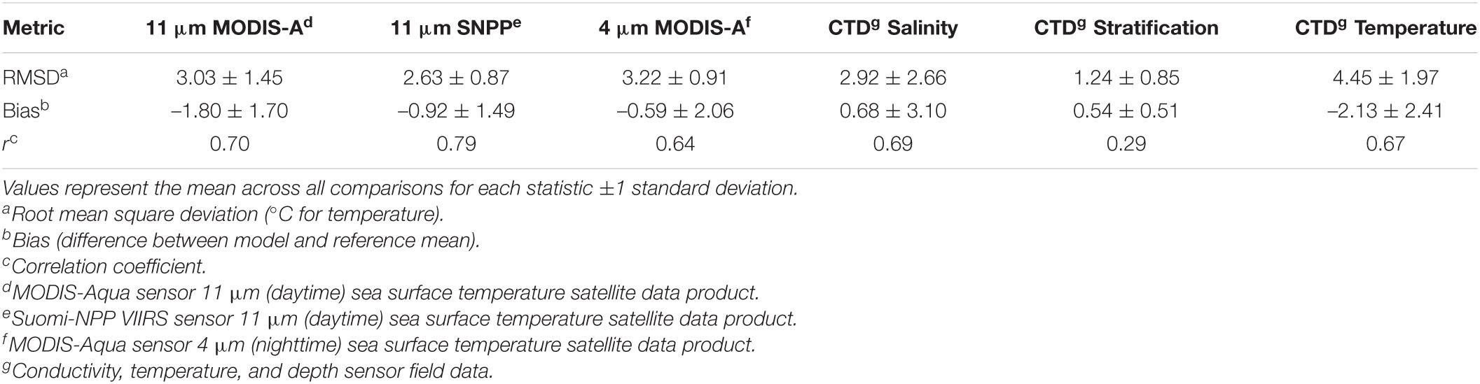
YukonFVCOM has a good SST predictive capacity and relatively high inter-annual precision of estimating SST, especially in summer months, across all years (Figure 3). Overall, the model performance indicates that for most months the model is within 3°C of the observed average SST and model performance improves from spring into summer. There is a general cold bias in the model relative to satellite observations (mean of –1.2°C) but there is variance across seasons and sensors (Table 2). 4 μm SST matchups were substantially less biased than 11 μm MODIS-A and SNPP observations (–0.59° vs –1.80° and –0.92°) indicating that the bulk heating and cooling into the ocean is well captured. This is because 4 μm SST is measured at night and is therefore more representative of overall heat content and not as susceptible to diurnal temperature variance of the surface skin layer. Performance bias improves from spring into summer across sensors, with improvements from –3.01° to –0.99° for 11 μm MODIS-A, –1.33° to +0.90° for 4 μm MODIS-A, and –1.53° to –0.51° for 11 μm SNPP. Each sensor has a uRMSD < –2.5° for the spring months, indicating the model was more spatially uniform relative to observations. uRMSD improves substantially after June, especially for 11 μm MODIS-A and SNPP comparison (uRMSD = –0.08° and –0.81°, respectively). Jia and Mennet (2020) found that MODIS-A SST had a mean bias of –0.57°C across the Arctic when compared to in-water observations, which suggests that as waters warm from spring into summer, YukonFVCOM predictive capacity improves to be substantially less biased. Overall, the relatively low bias as SST increased and the ability for YukonFVCOM to more closely match with the 4μm SST indicates that the bulk formulations related to heating and cooling can capture the first order temperature variance in the model domain.

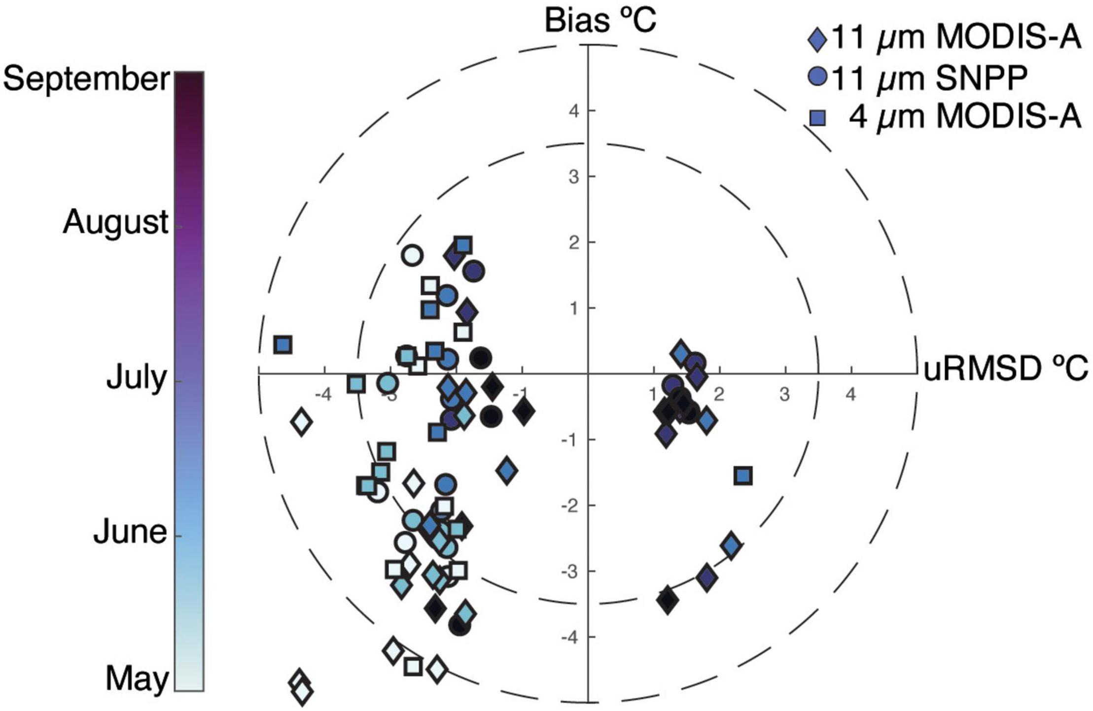
Figure 3. Target diagram for each year of the 7 model run years (2004–2005 and 2015–2019) for 11 μm sea surface temperature for MODIS-Aqua (all years) and Suomi-NPP (2015–2019) observed SST (SST) compared with the FVCOM model predicted SST and 4 μm (night time) SST which was only acquired in May–July for each year from the MODIS-Aqua instrument. Negative bias indicates a colder model prediction relative to the observed, while negative unbiased root mean square deviation (uRMSD) indicates less variability in the model prediction vs. observed. The sign of the uRMSD is determined by the sign of the difference of the standard deviation of the predictions and observations (Jolliff et al., 2009).

Table 2. Statistical metrics used to generate target diagrams (Figures 3, 4).

The parameterization for horizontal and vertical diffusion was matched to the parameters from an ideal river plume simulation (Chen et al., 2013) and was kept constant between model years, although individual tuning for each year may be needed to achieve optimal solutions. In addition, the specific heat capacity of water used in the COARE2.6 algorithm is held constant at that of seawater although in reality it changes with salinity. To further improve the temperature and salinity predictions, fine parameter tuning for each year and updating the heating algorithm to have a variable specific heat capacity is likely necessary, in addition to using real-time model predicted boundary forcing from a global model. Developments are currently under way to implement the 1/12° global HYCOM model (Smedstad et al., 2008) as the open boundary T and S, rather than climatological forcing, in years when the simulations are available. While the contribution of temperature to density within the plume is likely small due to the large salinity gradients, a future detailed analysis on model temperature is warranted to better understand the physical forcing that may not be well represented in the model formulations. Future simulations that represent sea ice formation and melting will likely impact the early springtime temperature and density fields which may have residual effects into May. This would be crucial to better understand how coastal temperature may have varied in the past and may vary into the future in the northern Bering Sea as seasonal sea ice continues to decline.

Model Comparison With in-situ Temperature and Salinity Profiles and Tidal Elevation

Like the satellite SST, the model generally has a cold bias (–2.44°C) in temperature profiles and the bias decreases as temperature increases (Figure 4A). The cold bias is mainly due to an underprediction of temperature in the bottom half of the water column (bias = –5.01°C) while surface waters agree well with observations (bias = 0.13°C). The mean uRMSD of 3.20 indicates that temperature stratification is slightly greater in the model than the observations. Coupled with the greater bias in the bottom water, this indicates the temperature stratification is likely overpredicted and vertical heat transfer is underpredicted in YukonFVCOM. Salinity comparisons indicate that YukonFVCOM can simulate the salinity field quite well across years, with mean bias of 0.35 and only slight differences in bias between the surface (–0.76) and bottom (1.47) salinity. The low total bias indicates that salinity variability and stratification in the plume and beyond is well captured. Model results are encouragingly strong along the RSWQ2019 transect which crosses the plume water, with most of the locations with the strongest stratification (yellow and green stars in Figure 4B) showing little bias. Coupled with the temperature comparison, YukonFVCOM reasonably represented the salinity distribution and stratification from the plume into Norton Sound.

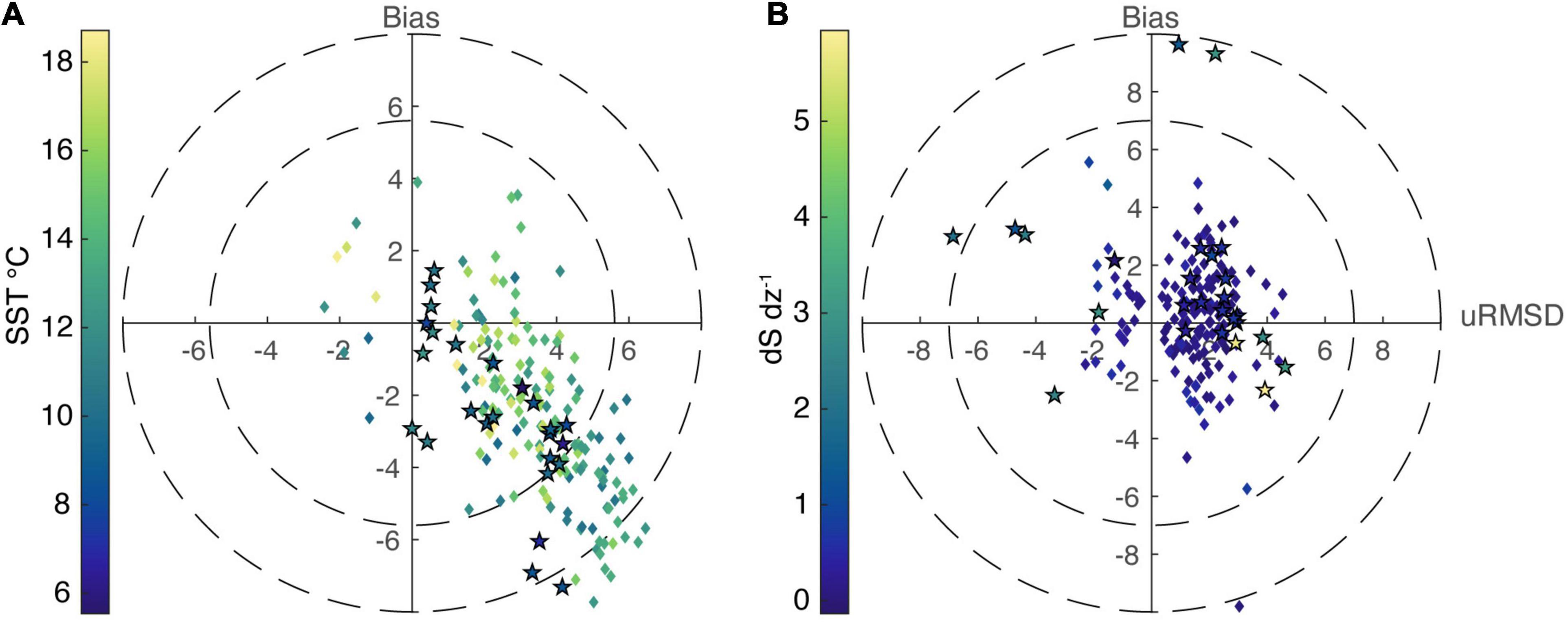
Figure 4. Target diagrams comparing model results with all CTD vertical data collected for (A) temperature profiles and (B) salinity profiles at the locations in Figure 1. Comparisons were made by matching the closest model-observed points in time (daily averaged model output), space, and depth. Diamonds represent profile comparisons at ADF&G stations in Norton Sound and stars represent values collected on the RSWQ 2019 Norton Sound-Yukon plume cruise. The coloring of each marker indicated by the color bars to the left of each panel represents the sea surface temperature (SST) and depth averaged salinity stratification (dS dz^–1) at the time of collection.

The unfiltered modeled and verified sea surface elevation values were well correlated across all years at Nome, AK (Supplementary Figure 4) and showed especially strong agreement for the tide station at Unalakleet at the interior edge of Norton Sound (Supplementary Figure 5). Near the model boundary at Nome, there was some difficulty in capturing high water events due the boundary SSH forcing constructed using the TPXO tidal predictions rather than a dynamically modeled product that accounts for SSH variation due to atmospheric effects. However, the strong performance at Unalakleet shows the YukonFVCOM model’s ability to simulate atmospheric induced SSH changes across years and seasons, with a mean Nash-Sutcliffe model efficiency of 0.54 and a mean correlation coefficient of 0.7 (Supplementary Table 1). Future implementations that utilize a global model product that can incorporate dynamic atmospheric effects will allow for a more realistic representation of open boundary SSH.

Mean Hydrographic Variability

Average hydrographic features from May to July for all 7 years indicate spatial variability that is relatively typical for a large northern hemisphere river plume (Figure 5). Surface salinity varied from 0 continuously around the Yukon delta up to ∼33 at the open ocean boundary toward the Bering Strait (Figure 5A). Salinity in Norton Sound was indicative of an estuarine environment with relatively low (<30) surface salinity and stratification persistent throughout the sound. The modeled salinity features are similar to surveys that were further out in Norton Sound toward the Bering Strait, with values near 30–32 at the surface and weakening vertical stratification further into the ocean (Dean et al., 1989). The freshwater plume extended furthest into the ocean at the outflow of the southern river mouth where the majority of freshwater exited the delta. The bulge at the south mouth is consistent with a prototypical plume (Horner-Devine et al., 2015) and is very similar to dynamics seen in other large western North American rivers such as the Columbia River (Hickey et al., 1998).

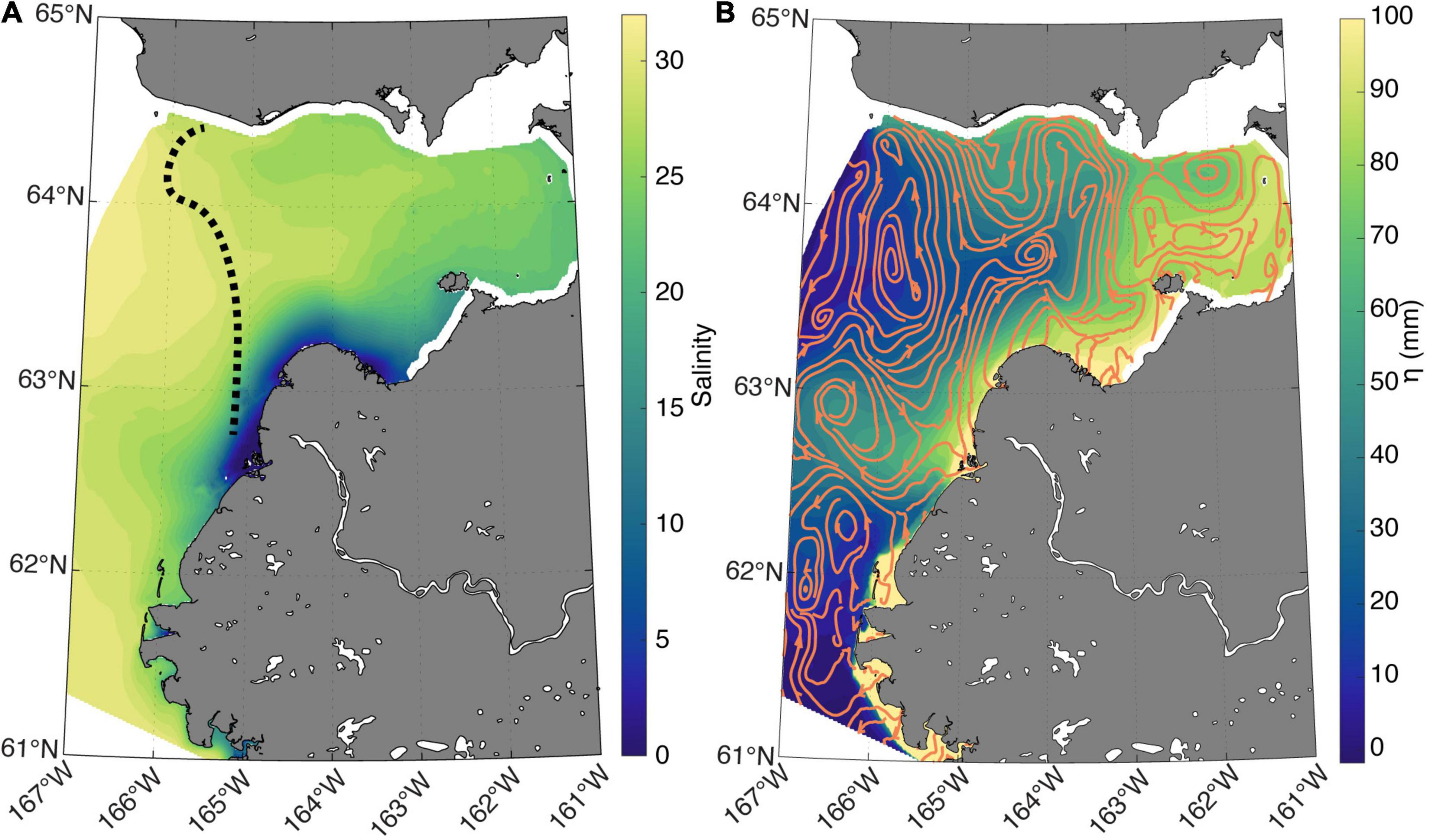
Figure 5. Seven-year depth averaged May-July (A) salinity and (B) sea surface height (η) with the vertically averaged velocity field represented by the stream lines. The stream lines were derived using the built-in MATLAB function streamslice.m.

The vertically averaged velocity and sea surface height (η) show a pressure gradient from the delta and eastern edge of Norton Sound sloping toward the Bering Strait, in addition to a prominent eddy that persists at the outflow near the southern mouth of the delta (Figure 5B). The anti-cyclonic eddy off the coast of the south mouth coincides with an area of elevated η that extends from the south mouth toward the model boundary and continental shelf. Along the coast north into Norton Sound, there is a strong northeastward current that pulls water from the eddy region (the bulge) and river delta toward the east side of Norton Sound. Velocity is predominantly northward bringing plume waters toward the north coast of Norton Sound where a strong coastal westward jet pushes water toward Bering Strait. This flow pattern toward the Bering Strait has been previously documented in studies looking at sediment distribution (Dupré, 1980) and a recent Saildrone survey also exhibited evidence of the bulge extending toward the west with the mean flow pulling freshwater back across the face of the delta toward the east into Norton Sound (Cokelet et al., 2015). The qualitative comparison of the YukonFVCOM mean flow and the historical surveys give confidence that the hydrographic patterns exhibited by YukonFVCOM are realistically capturing the flow patterns in the coastal ocean and that the model is a useful tool to analyze controls on the hydrographic variability under differential external forcing conditions.

The plume bulge eddy and coastal currents are typical of large river plumes where the balance between the Earth’s rotation and the buoyancy and pressure gradient drives transport along the coast northward into Norton Sound (Hickey et al., 1998; Hetland, 2005). It has been shown that along shore flow of river plumes is governed by the rotation of the earth on longer time scales (Garvine, 1987; Yankovsky and Chapman, 1997) and that large river plumes with small estuaries typically exhibit the bulge feature at the river outflow (Yankovsky and Chapman, 1997; Horner-Devine et al., 2015). The Yukon plume is no exception, and plume dynamics related to the Earth’s rotation such as bulge distribution and coastal current velocity are likely enhanced due to the high latitude. Shorter term variation due to wind forcing that undoubtedly affects river plume dynamics and distribution will be explored further in the following section.

Interannual Variation in Plume Dynamics

Salinity was more horizontally uniform relative to u and v currents with a greater average semi-variogram range (63.1 ± 4.4 km) (mean ± standard deviation, σ hereafter) and there were relatively similar values across all years, indicated by the similarity of the variograms (Supplementary Figure 6A) and the low relative σ of the range and sill (Table 3). u velocity was more spatially uniform (range = 32.5 ± 13.7 km) but had much greater interannual variation relative to v velocity (range = 19.2 ± 2.0 km) indicated by the greater σ. The small standard deviation (relative to the mean) in both salinity and v velocity indicate that interannual variability was relatively small and spatial variability of these quantities was consistent across the years even though there were substantial differences in discharge. Contrarily, the u velocity field had greater interannual variability, with 2005 and 2016 standing out as outliers with a much more uniform (larger range) u velocity field (Table 3), indicated by the shallower slope in the respective curves (Supplementary Figure 6B). These 2 years had the largest cumulative discharge (247 and 243 km³, respectively) in the 37-year gauge record, suggesting that river flow may be an important predictor of u current velocity within the plume.

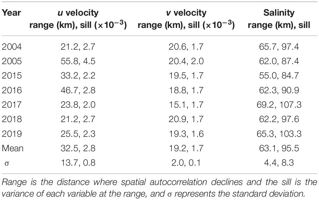
Table 3. Metrics used to model the variograms for the annual average May–July u and v surface velocity and salinity.

Comparisons of the semi-variogram range for u, v, and salinity with river discharge and wind velocity show that wind velocity and river discharge can have differential effects on river plume dynamics. Cumulative spring river discharge was not correlated with salinity or v semi-variogram range, but the u velocity range was significantly (p < 0.05) related to the cumulative discharge (Figure 6A). High discharge decreased the spatial variance of the u velocity field indicating cumulative spring discharge is likely a forcing factor that affects variance in the u velocity across years. Changes in plume velocity and salinity were not correlated with E–W wind velocity (Figure 6B), but there was a significant correlation between v current velocity range and N–S wind (Figure 6C). These results show that across years: (1) u current velocity variation is related to the total amount of freshwater entering the ocean; (2) v current velocity variation was related to the average N–S wind in the springtime across years; and (3) E–W wind velocity variance was not correlated to the mean salinity or current spatial variance. Wind velocity was typically northerly (wind toward the south from the Arctic Ocean; Supplementary Figure 2) and stronger northerly winds correlated with a decrease in the spatial variance in the v velocity field. Finally, salinity spatial variance was un-correlated with the three forcing variables analyzed here, and salinity was relatively stable across the 7 years (Table 3).

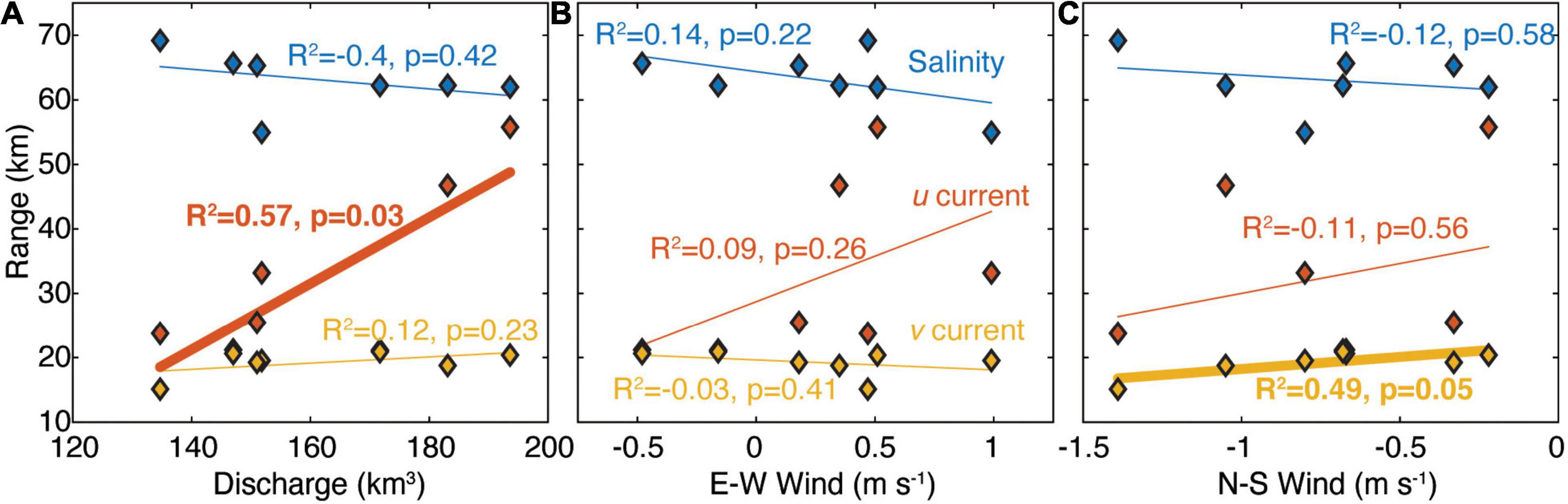
Figure 6. Semi-variogram range for salinity, u (west–east), and v (south–north) current velocity as a function of (A) Yukon discharge, (B) East–west wind velocity and (C) North–south wind velocity. R² and p values are the coefficient of covariance and significance level determined by an ordinary least-squares linear regression. Bold values and lines are statistically significant (p ≤ 0.05). Note the axis for E–W and N–S wind have different values.

Velocity Structure in the Plume Across Norton Sound

Along the transect that follows the sampled cruise track from 2019 (Figure 5A), the mean u and v velocity fields were extracted for May–July across all years and the u and v velocity fields were averaged (n = 21; Figures 7A,B). To orient the reader, positive velocity is eastward or northward out of the page (u) or toward the right (v), while negative values are westward and southward into the page or toward the left. u velocity exhibited a strong rotational flow along the transect near the delta in the low salinity water of the plume with strong westward flow near the south river mouth and eastward flow ∼75 km down the transect to the north (Figure 7A). This corresponds with the anticyclonic eddy observed in the streamline velocity field in Figure 5A, along with the elevated η in the bulge region. Further into Norton Sound > 100 km away from the river mouth, the u velocity shifted from strong eastward to weakly westward with the mean flow out of Norton Sound toward the open ocean. The strong westward coastal jet along the north coast of Norton Sound observed in the surface velocity extended almost 20 m into the water column before dissipating and reversing eastward near the sea floor. The model does not include other small river and stream systems around Norton Sound, therefore the buoyancy driven flow patterns are solely due to the interaction of Yukon River and oceanic water. The opposing flow at the north edge of Norton Sound is indicative of two-layer circulation showing the estuarine nature of Norton Sound.

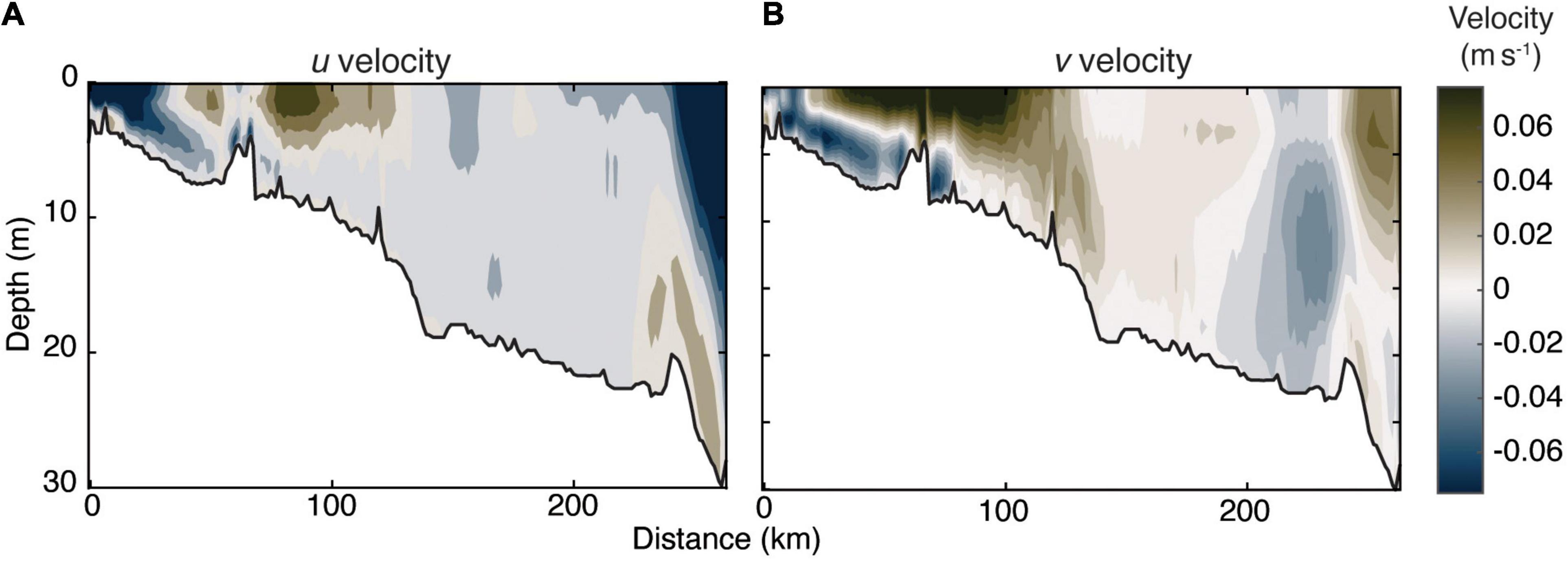
Figure 7. Seven-year averaged May–July (A) u (west–east) and (B) v (south–north) current velocity along the transect that follows the western cruise track from the RSWQ June 2019 cruise.

v Velocity within the plume exhibited strong two-layer circulation up to ∼100 km away from the river mouth (Figure 7B). The velocity remains weakly northward before strengthening near the north coast where the coastal jet turns toward the northwest and the Bering Strait. v Velocity began to reverse toward the south >200 km down-transect at >10 m deep which coincided with the bottom u current flowing back into Norton Sound. Combined with the u current field and the depth averaged velocity field (Figure 5B), there was a two-layer eddy with southwestward flow at the mouth, and northeastward flow further down transect into Norton Sound. There was also a topographic effect in the north-south direction where along-transect velocity had a persistent downwelling of strong surface velocity into the interior of the water column to >10 m of depth ∼125 km from the river mouth. The presence of these distinct features such as the anticyclonic eddy and two-layer circulation provide further evidence that the Yukon plume behaves as a prototypical river plume (Horner-Devine et al., 2015) and that Norton Sound has a density driven estuarine circulation. Analyzing the behavior of the Yukon plume during specific events can be potentially applicable for other high latitude rivers entering the ocean in shallow and broad shelf waters.

Plume Structure Is Strongly Influenced by Wind Velocity

There is a correlative link between north-south wind and surface ocean v velocity which manifested in the spatial variance analysis presented in Figure 6C, but the spatial variance of salinity appears to be unaffected by wind velocity when averaged over the freshet period for each year. However, short-term strong wind events likely affect the spatial density distribution and velocity fields within the plume, which has been documented from both field observations and numerical modeling studies in various coastal systems (Fong and Geyer, 2001; Whitney and Garvine, 2005; Horner-Devine et al., 2015). Wind storm events were predominantly southwesterly (toward the northeast) from the Bering Sea toward the North American Arctic land mass. The average duration of southwesterly storms was substantially longer (5.43 days; Table 4) than other directions, which averaged 2–3 days per event, and southwesterly wind events were the only type to occur in all 7 years. In this region, north winds are characterized as “upwelling” and south winds are characterized as “downwelling” due to the overall effect of the wind on the Ekman transport of coastal water. The strongest average wind magnitude during storms occurred from the northwest from the Arctic Ocean across Norton Sound with a mean velocity of 5.4 ± 0.85 m s^–1 (Table 4). Overall, southwesterly wind events tended to occur earlier in the year with an average date of July 16; the other directional events tended to occur later into the summer in August and September when flow is typically lower (Table 4). Although there was substantial variability in wind direction throughout each year, the average non-storm wind blew from the Arctic over Norton Sound to the south but shifted year to year between westerly and easterly trajectories (Table 1 and Supplementary Figure 2).

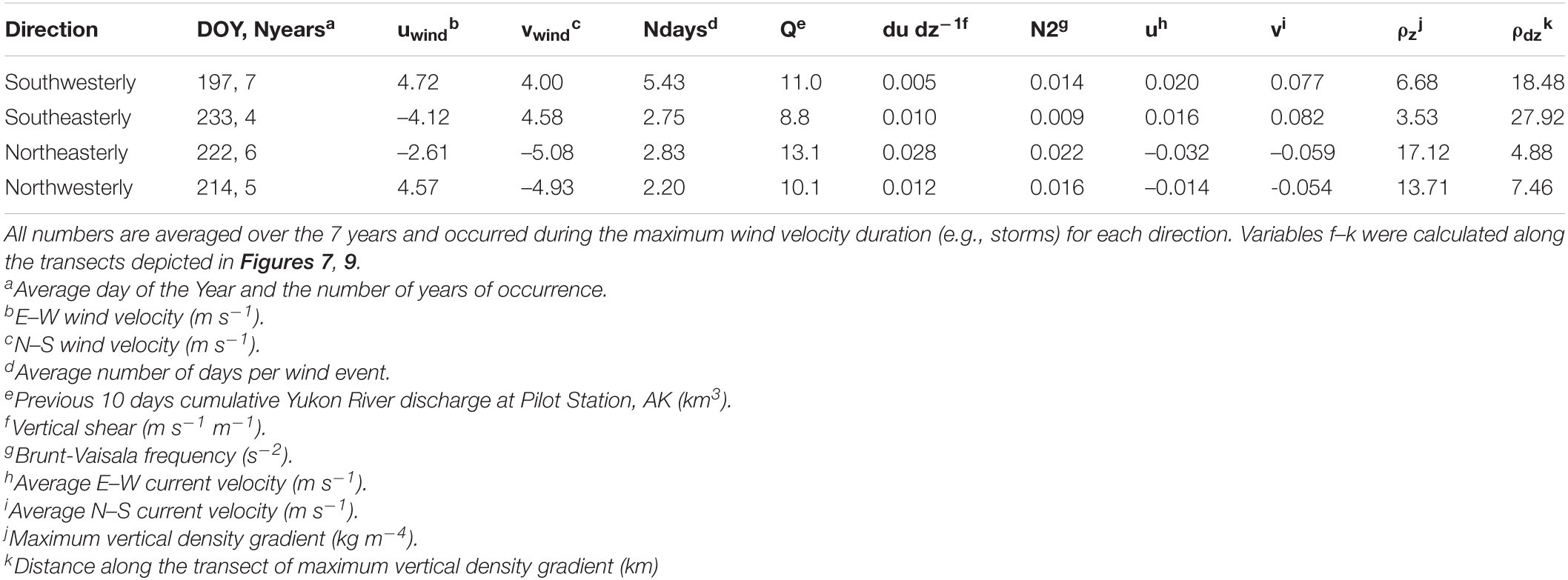
Table 4. Parameters related to wind and current velocity and river plume extent and strength.

The coastal currents differed substantially depending on the prevailing winds during storms. Analysis of the plume velocity during these wind events revealed that southerly (downwelling; Figures 8A,B) winds and northerly (upwelling; Figures 8C,D) winds substantially altered the depth-averaged current velocity. Downwelling wind pushed water near the coast toward the river delta and eastern edge of Norton Sound enhancing the mean flow pattern across the sound and toward the Bering Strait. The downwelling winds enhanced the northeastward flow with >20 cm s^–1 flow in the surface toward the northeast and northward surface flow deepening > 10 m into the water column over 150 km away from the south river mouth (Figures 9A,B). The mean u and v velocity was much greater than the annual average while occurring in the same direction showing that the downwelling winds substantially enhanced the plume circulation. This coincided with a large increase in η near the delta and in Norton Sound which likely enhanced the mean transport northwestward along the toward the Bering Strait down the pressure gradient. However, the prototypical bulge seen in the annual mean flow was largely diminished (Figures 8A,B) with the enhanced northward transport. The enhancement of velocity at depth away from the plume suggests that the currents could transport riverine material > 100 km offshore into deeper Norton Sound waters. The average current velocity <125 km from shore was 13.0 cm s^–1 in the southerly wind events; a water mass leaving the southern end of the transect would take 11.1 days to be transported 125 km into the interior of Norton Sound, on average.

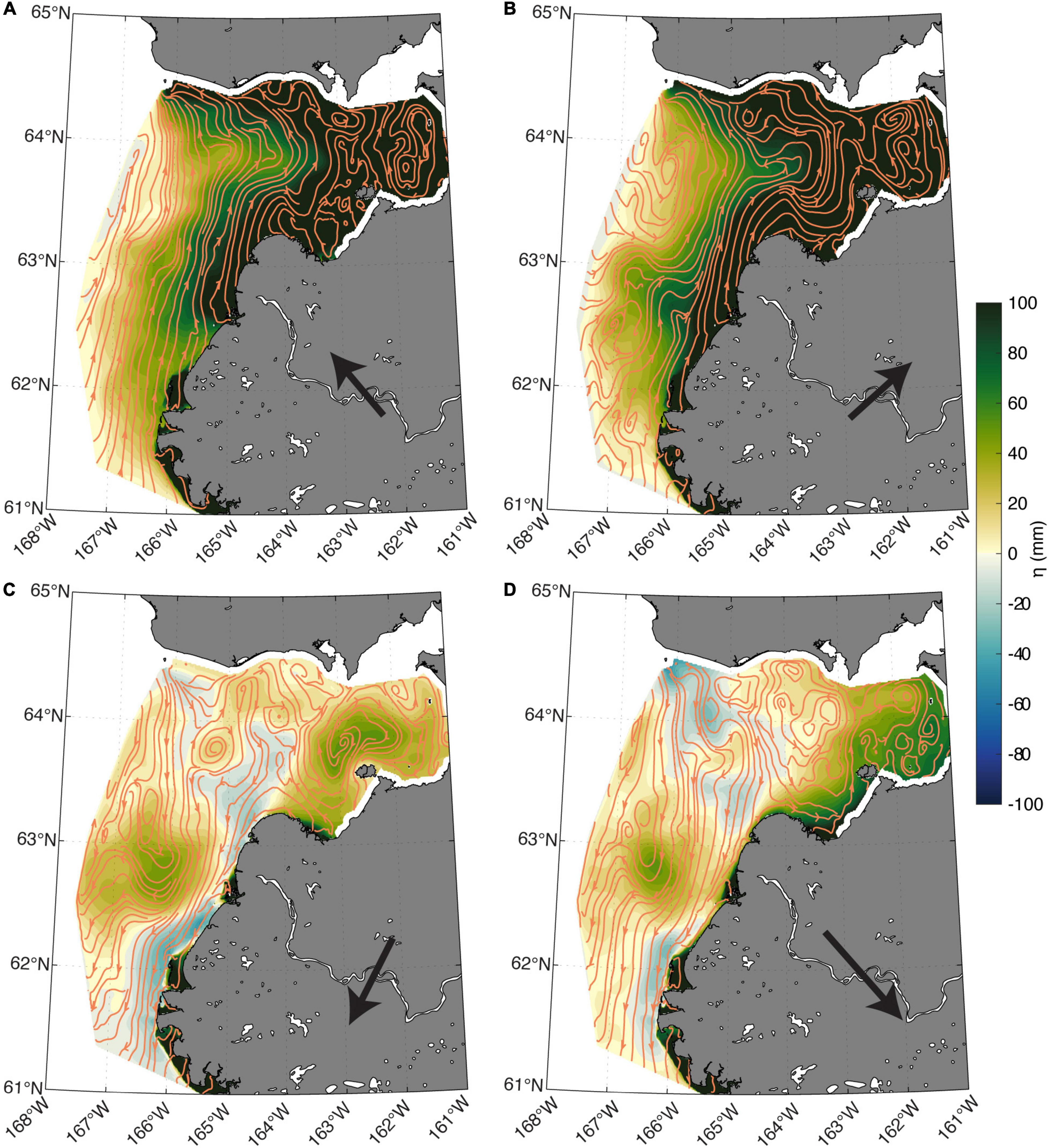
Figure 8. Seven-year averaged surface height (η) for each year’s longest duration wind event for (A) southeasterly, (b) southwesterly, (C) northeasterly, and (D) northwesterly. The streamlines are estimated from the depth-averaged u and v velocity fields and the arrows show the mean wind for each pattern.

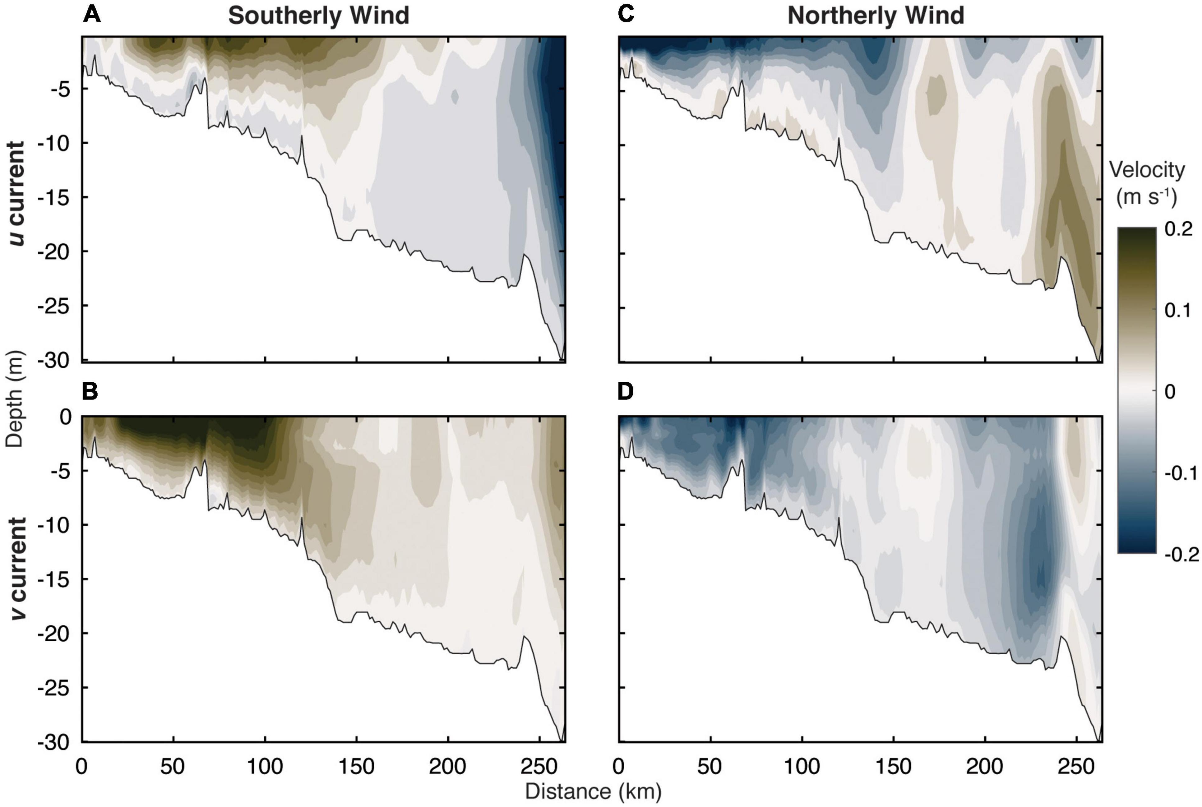
Figure 9. Average southerly wind event (A) u and (B) v current velocity, and average northerly wind event (C) u and (D) v current velocity. Positive u is to the east (out of the page) and positive v is to the north (down the transect).

Upwelling winds from the north drove the depth averaged flow to completely reversed with currents moving southward against the northward flow typically seen (Figures 8C,D). There was a southwestward flow with a strong surface current in the nearshore < 150 km from the mouth pushing water toward the west in the near river plume region (Figure 9C). Strong westward currents (>20 cm s^–1) were confined to the upper 5 m of the water column within the plume and combine with weaker and more vertically homogenous southward currents (Figure 9D). Mean vertical shear was greatest in the northeasterly wind events at 2.8 cm s^–1 m^–1 (Table 4), compared to the southwesterly winds where the mean vertical velocity was more uniform (0.5 cm s^–1m^–1). The v current field has reversed and there is now a persistent southward flow at depth in Norton Sound 225 km down transect. Rather than the typical persistent coastal current along the north coast Norton Sound, an eastward current occurred at depth (Figure 9C), pulling water from the bottom near the Bering Strait into Norton Sound where it is advected southward back toward the river plume. The enhanced two-layer flow in Norton Sound with multiple regions of divergence in the v velocity field is indicative of strong upwelling: water is moving into Norton Sound along the bottom pushing deeper water from the Bering Strait shown in southwestward through Norton Sound.

The upwelling wind substantially depressed the elevated η along the coast (Figure 8D). The elevated η in the bulge region remained a substantial hydrographic feature with the velocity field still exhibiting some rotation around this area of high pressure before continuing toward the south in the direction of the wind field. Surprisingly, the upwelling wind driven mean current magnitude <125 km from the river mouth was 11.2 cm s^–1 southward, only slightly less than 13.0 cm s^–1 northward from the downwelling wind (Figure 9D). Wind was the predominant factor shifting the mean flow of water with downwelling winds enhancing the mean flow and upwelling winds shifting the flow in the opposite direction and transporting water southward away from the region of typical plume dispersion. The complete diminishment of the two-layer circulation and persistent southwestward flow within the plume during upwelling winds show that strong wind cannot only affect the mixing in the far field of the plume (as described in Horner-Devine et al., 2015) but can also drive flow shifts in the near field at the plume front and at the outflow of the river.

Fong and Geyer (2001) showed that upwelling winds will diminish along shore flow in the mean plume direction and the Yukon plume not only exhibited a diminished dominant northeastward flow pattern but a complete reversal during upwelling events throughout the water column. The effect of wind forcing on the horizontal velocity occurred throughout the river plume, not just down transect away from the front in the far field. These flow patterns indicate that material that is transported from the river such as sediment and dissolved matter will be deposited and distributed in much different locations depending on the direction of the wind. Southerly winds transport a greater portion of plume water northeastward into Norton Sound at a much faster rate and deeper into the interior of the water column, potentially depositing finer sediment further offshore in deeper water in Norton Sound. Upwelling winds do the opposite, likely increasing coastal water residence time in the nearshore region before being transported through Norton Sound and toward the Bering Strait after wind slackens, and buoyancy and rotational flow begin to dominate again. This would likely increase sediment deposition in the near field adjacent to the delta and offshore toward the west. Importantly, increased residence time of riverine water and the addition of upwelled deeper water at the coast will likely alter biogeochemical cycles such as increasing the breakdown of riverine organic matter and providing more nutrients to the surface ocean from depth. While in-water sampling would be dangerous and difficult during high wind-events, YukonFVCOM can provide a qualitative estimate of the spatial distribution of plume water for any scenario and provide a first-order estimate of where the plume frontal regions occur in short time frames.

Stratification as quantified by N² and vertical velocity (ω) within the plume had a similar, expected, response as the horizontal velocity field during wind events (Figure 10). Downwelling winds broadened the low-density plume waters northward (Figures 10A,B), and enhanced downward vertical velocity (Figures 10C,D). However, not all downwelling winds are the same with southeasterly and southwesterly winds showing a much different response in the magnitude of stratification and density. Southwesterly winds exhibited a much higher degree of stratification and lower density plume water extended further offshore as isopycnals bent upward (Figure 10B), and there was much greater downward vertical velocity in the near- and mid-field regions (Figure 10D). The downward velocity coincides with the deepened northeastward flow (Figures 9A,B) showing that plume water was advected further offshore and at a greater depth into the interior of Norton Sound relative to the mean. Stratification was greatest near the sea floor <50 km down transect with a relatively uniform and incremental increase in density up to 100 km. Southeasterly winds drove vertical shear to be ∼2× greater than southwesterly winds while the Brunt-Vaisala frequency was 36% less (Table 4) even though the southerly wind component was relatively similar to southwesterly winds (4.58 vs. 4.00 m s^–1). This suggests that the east-west wind velocity vector component contributed more to the variance in the current velocity and density fields during downwelling winds and that westerly wind components increased stratification and diminished mixing along the transect.

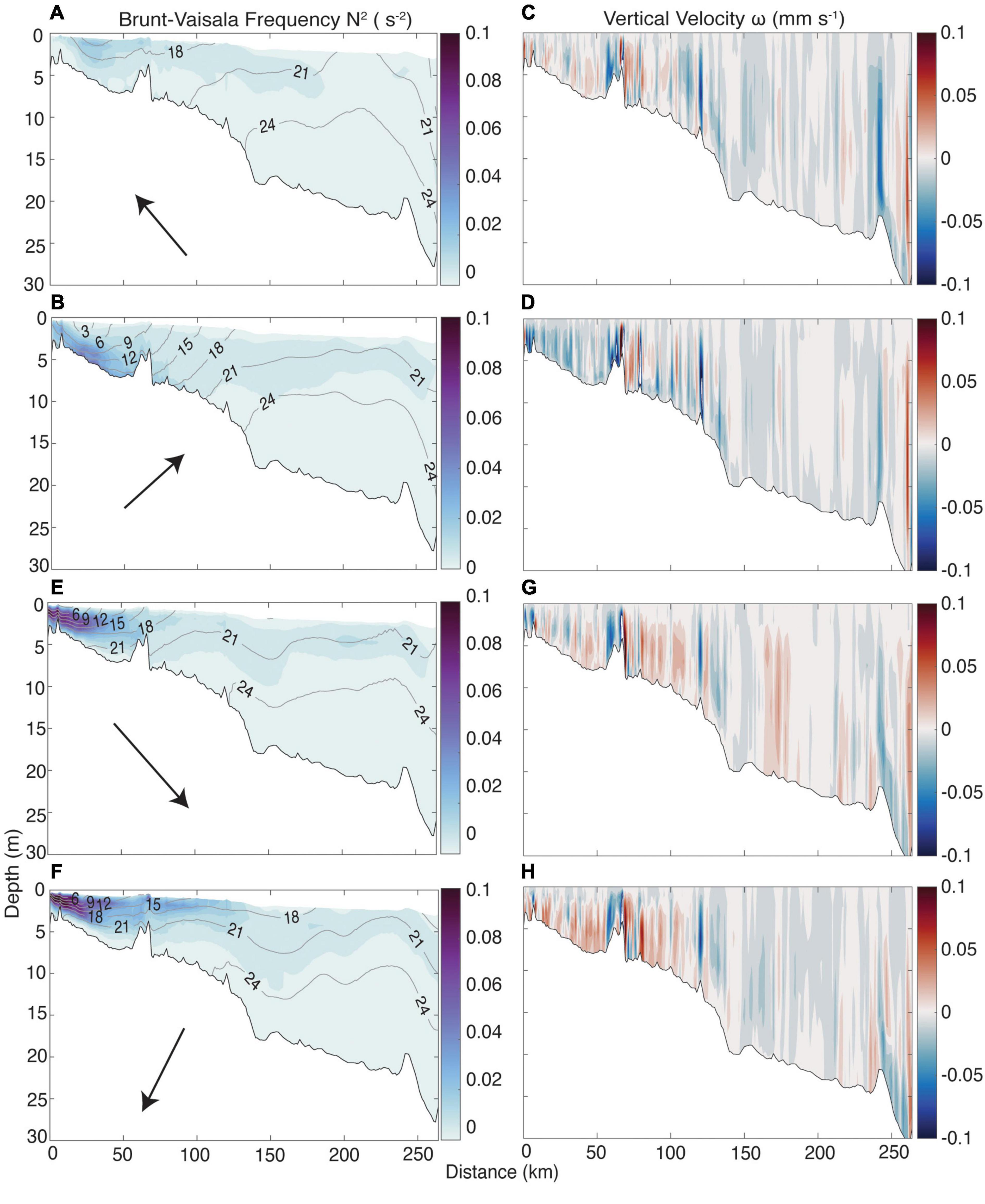
Figure 10. Mean vertical Brunt-Vaisala frequency (N2) (first column) and vertical velocity (ω) (second column) for the mean of the southeasterly (A,C), southwesterly (B,D), northwesterly (E,G), and northeasterly (F,H) wind events averaged across all years. The contour lines and labels in the first column depict the σθ (kg m-3) for each extracted transect. The arrows in the first column represent the average direction and magnitude of the wind for each row of plots, relative to north.

Upwelling winds shoaled the depth of greatest stratification toward the surface and near the plume outflow (Figures 10E,F) and drove upward transport of water within 125 km of the plume outflow (Figures 10G,H). The maximum vertical density gradients increased to 17.1 and 13.7 kg m^–4 for northeasterly and northwesterly wind events, compared to 6.68 and 3.53 kg m^–4 during downwelling wind events. The maximum vertical stratification occurred 4.9 and 7.5 km down the transect, compared to 18.5 and 27.9 km in the downwelling winds (Table 4). These circulation and stratification patterns show that upwelling-favorable winds increased river water retention near the surface and toward the southwest at the main river outflow by increasing stratification and shoaling the pycnocline. These flow patterns suggest that river water suspended material processing and deposition may increase in the near field while dissolved tracers may be confined to the near surface allowing for transport further offshore in surface waters toward the southwest away from the direction of the mean flow.

Finally, the difference in depth-averaged salinity between downwelling and upwelling winds shows the substantial spatial difference in plume water distribution under variable wind (Figure 11). The regions at the main outflow of the river at the south mouth and throughout the delta have a difference of >10 salinity with fresher water throughout the north edge of the delta during downwelling, coinciding with the enhanced northward transport. Downwelling winds also appeared to increase transport of more oceanic water into Norton Sound which logically follows the downward advection of water and replacement by marine water at the surface due to mass balance. Overall, upwelling and downwelling winds have a substantial effect on the short term spatial distribution of plume water throughout the region and can largely determine where the majority of river water is concentrated in the coastal ocean on short time scales.

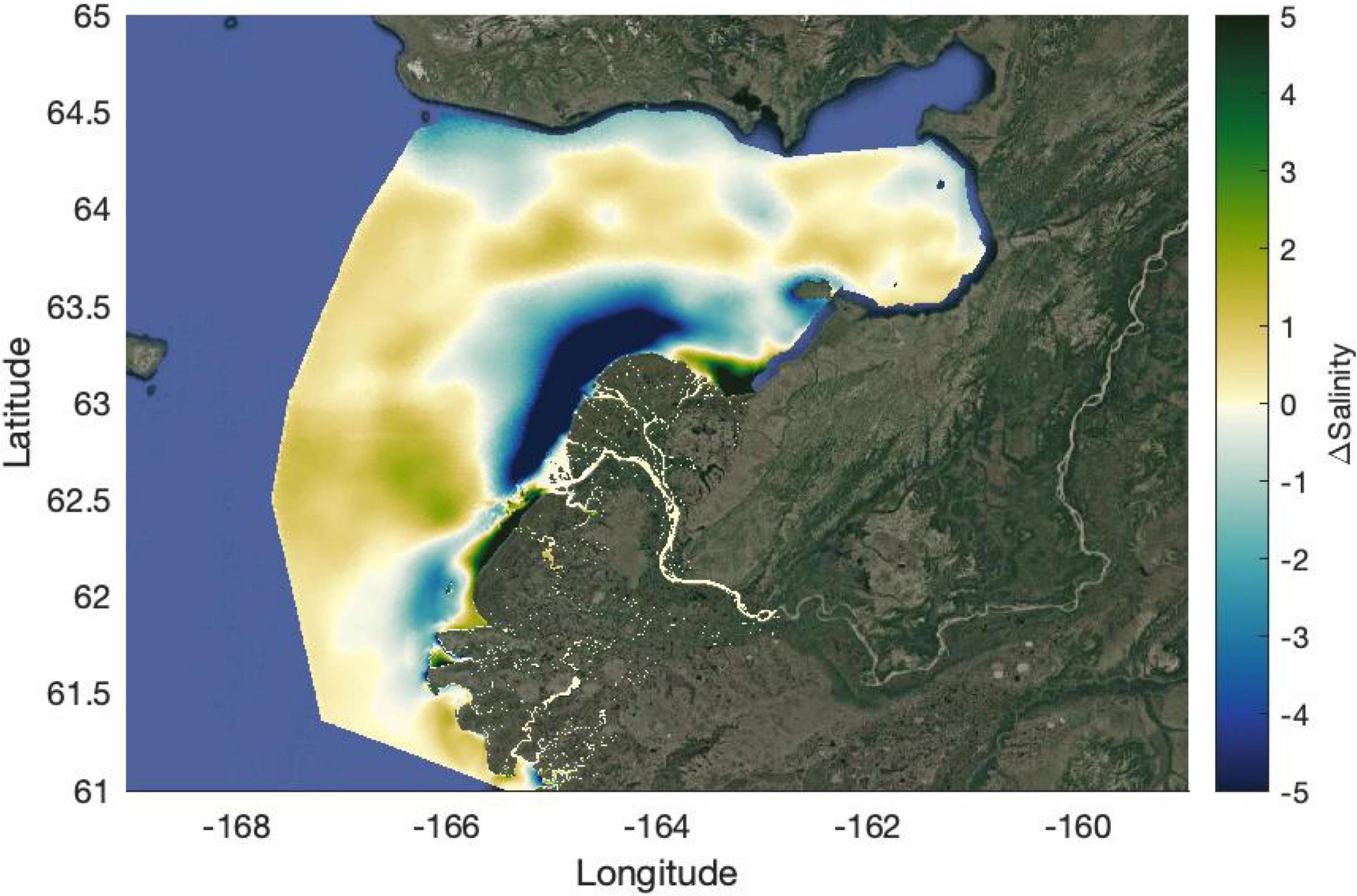
Figure 11. The difference in the depth averaged salinity between the mean of the downwelling and upwelling wind events. Positive values indicated the downwelling has greater salinity and negative values indicate upwelling has greater salinity. Background image was created using the MATLAB function Plot_Google_Map.m (Bar-Yehuda, 2021).

Implications for Plume-Ocean Biogeochemistry

Wind direction has a strong influence on the plume strength and distribution in the coastal ocean which will determine the time and space scales of riverine material processing during coastal ocean transport. Depending on the interplay between river flow and wind velocity, material can be confined to the coast or transported far offshore which will alter regional sediment and dissolved matter biogeochemistry. Further analysis of long term model predictions in the context of inter-decadal weather variation could show if changes in regional wind patterns may effect plume dispersion on longer time scales and in the context of the changing Arctic climate. This will be key for generalizing how increasing river flow in the future will manifest in the plume impacts on coastal biogeochemical processes coupled with changes in regional atmospheric forcing.

Key processes such as sediment deposition, dissolved organic matter remineralization, and nutrient dispersion will therefore be governed by the wind forcing on the plume. Suspended sediment dynamics are difficult to characterize, especially in regions with strong coastal currents and a plume distribution that can vary by 100s of kilometers depending on the surface wind field. To characterize sediment deposition or resuspension in the Yukon Plume, a sampling scheme must be efficiently employed that can capture the full spatial variability of the plume in the near- and mid-field regions, independent of wind direction. By understanding the degree to which specific wind events determine the plume distribution, sampling schemes can be better informed to maximize effort where and when samples are collected. For example, if there was a strong upwelling event prior to a field expedition, it would be pertinent to focus sampling efforts near the mouth of the river and toward the south and southwest to capture the rapidly sinking/freshly deposited riverine sediment in the likely location they would be distributed.

Another important process in the transition from plume-to-ocean in the mid-field region of the plume is the mixing of freshwater derived dissolved organic carbon and marine water with high ionic strength. At this transition, high molecular weight compounds tend to precipitate out or bind with suspended matter into large colloids in a process known as flocculation (e.g., Sholkovitz et al., 1978; Verney et al., 2009; Asmala et al., 2014). External factors affecting the location of the plume transition zone will also affect flocculation as the plume front shifts under variable forcing. Capturing flocculation spatial patterns and rates of formation in the Yukon Plume and other large rivers is a high priority due to the very high sediment and organic loads to the coastal ocean. The strong seasonality and rapid transition from low to high flow during the freshet makes targeted sampling difficult without information on the real-time dynamics of the plume. However, representative and comprehensive sampling is critical to develop process-based experiments that estimate biogeochemical processes at the plume-ocean interface which can then inform biogeochemical models of these coastal regions. The wind patterns over the plume region before and during sampling can be used to qualitatively predict where the dominant plume front will occur and thus where sampling should be focused. While running the YukonFVCOM model in real time on a supercomputer is not configured (yet), combining the general knowledge of plume distribution in relation to wind forcing with remote measurements of ocean properties via satellites can lead to the efficient deployment of resources in this difficult to access environment. Finally, the characterization of the mean flow field will allow for future deployment of autonomous sampling platforms into locations to maximize sampling return. This is key in such a remote location that is rapidly undergoing climate change and where in-water observations are particularly sparse.

Data Availability Statement

The FVCOM model output used in this study along with some post-processing scripts can be found at https://portal.nccs.nasa.gov/datashare/yukonriver/. The FVCOM source code version 4.3 is publicly available for download at http://fvcom.smast.umassd.edu/fvcom/. The river forcing for the Yukon River is available from the United States Geological Survey, the tidal prediction software is available at https://www.tpxo.net/global, the open boundary forcing is available through the World Ocean Atlas, and the model validation is available through the DAACs referenced in the main text.

Author Contributions

JC constructed the model under the advise and expertise of AM. AM contributed substantially to the curation and editing of the manuscript and advice during model construction and analysis. Both authors contributed to the article and approved the submitted version.

Funding

This work was solely funded under the US National Aeronautics and Space Administration.

Conflict of Interest

The authors declare that the research was conducted in the absence of any commercial or financial relationships that could be construed as a potential conflict of interest.

Publisher’s Note

All claims expressed in this article are solely those of the authors and do not necessarily represent those of their affiliated organizations, or those of the publisher, the editors and the reviewers. Any product that may be evaluated in this article, or claim that may be made by its manufacturer, is not guaranteed or endorsed by the publisher.

Acknowledgments

We would like to acknowledge the Alaska Department of Fish and Game (ADF&G) and specifically Jenefer Bell for providing the CTD data used for model validation/calibration in Norton Sound, and the NASA RSWQ2019 award #80NSSC18K0492 to P. J. Hernes, RGM Spencer, and M. Tzortziou (UC Davis) and under funded program 281945 to AM (NASA GSFC) that provided support to acquire CTD data along the cruise track in 2019. Thank you to Peter Hernes and Maria Tzortziou for helpful comments during the drafting of this manuscript. We also acknowledge Michael Novak for his leadership in the RSWQ2019 sampling effort and help with acquiring and processing data, and the NASA Center for Climate Simulation supercomputer Discover support team in help getting this model up and running and the allocation of resources they generously provide. Finally, we acknowledge the Native Alaskan village of Alakanuk for hosting us during our work in the Yukon Delta, especially Augusta Edmund and Captain Adam Boeckman of the Anchor Point for the Nome-Norton Sound portion of the RSWQ2019 field campaign. Thank you to two reviewers for helpful comments in improving this manuscript. The contribution of JC was primarily conducted under the NASA Postdoctoral Program, administered by Universities Space Research Association.

Supplementary Material

The Supplementary Material for this article can be found online at: https://www.frontiersin.org/articles/10.3389/fmars.2021.793217/full#supplementary-material

Footnotes

1. ^ https://nsidc.org/data/seaice_index
2. ^ http://nco.sourceforge.net/
3. ^ https://waterdata.usgs.gov/nwis/inventory/?site_no=15565447

References

Asmala, E., Bowers, D. G., Autio, R., Kaartokallio, H., and Thomas, D. N. (2014). Qualitative changes of riverine dissolved organic matter at low salinities due to flocculation. J. Geophys. Res. Biogeosci. 119, 1919–1933. doi: 10.1002/2014JG002722
Banas, N. S., MacCready, P., and Hickey, B. M. (2009). The columbia river plume as cross-shelf exporter and along-coast barrier. Continental Shelf Res. 29, 292–301. doi: 10.1016/j.csr.2008.03.011
Bar-Yehuda, Z. (2021). zoharby/plot_google_map. Availble online at: https://github.com/zoharby/plot_google_map, GitHub. (accessed December 13, 2021).
Chen, C., Beardsley, R. C., Cowles, G., Qi, J., Lai, Z., Gao, G., et al. (2013). An Unstructured grid, finite-Volume Community Ocean Model FVCOM user Manual, SMAST. UMASSD Technical Report-13-0701.
Chen, C., Gao, G., Zhang, Y., Beardsley, R. C., Lai, Z., Qi, J., et al. (2016). Circulation in the Arctic Ocean: results from a high-resolution coupled ice-sea nested global-FVCOM and Arctic-FVCOM system. Prog. Oceanogr. 141, 60–80. doi: 10.1016/j.pocean.2015.12.002
Clark, J. B., and Mannino, A. (2021). Preferential loss of Yukon river delta colored dissolved organic matter under nutrient replete conditions. Limnol. Oceanogr. 66, 1613–1626. doi: 10.1002/lno.11706
Cokelet, E. D., Meinig, C., Lawrence-Slavas, N., Stabeno, P. J., Mordy, C. W., Tabisola, H. M., et al. (2015). The Use of Saildrones to Examine Spring Conditions in the Bering Sea. Washington: OCEANS 2015 - MTS/IEEE, 1–7. doi: 10.23919/OCEANS.2015.7404357
Danielson, S. L., Ahkinga, O., Ashjian, C., Basyuk, E., Cooper, L. W., Eisner, L., et al. (2020). Manifestation and consequences of warming and altered heat fluxes over the Bering and Chukchi sea continental shelves. Deep Sea Res. Part II Top. Stud. Oceanogr. 177:104781. doi: 10.1016/j.dsr2.2020.104781
Dean, K. G., Mc Roy, C. P., Ahlniis, K., and Springer, A. (1989). The plume of the yukon river in relation to the oceanography of the bering sea. Remote Sensing Environ. 28, 75–84. doi: 10.1016/0034-4257(89)90106-5
Dornblaser, M. M., and Striegl, R. G. (2009). Suspended sediment and carbonate transport in the yukon river basin, alaska: fluxes and potential future responses to climate change. Water Resour. Rese. 45:7546. doi: 10.1029/2008wr007546
Dupré, W. R. (1980). Yukon Delta Coastal Processes Study. Houston, TX: Department of Geology, University of Houston.
Durocher, M., Requena, A., Burn, D. H., and Pellerin, J. (2019). Analysis of trends in annual streamflow to the Arctic Ocean. Hydrol. Proc. 33, 1143–1151. doi: 10.1002/hyp.13392
Egbert, G. D., and Erofeeva, S. Y. (2002). Efficient inverse modeling of barotropic ocean tides. J. Atmospheric Oceanic Technol. 19, 183–204. doi: 10.1175/1520-0426(2002)019<0183:EIMOBO>2.0.CO;2
Fairall, C. W., Bradley, E. F., Hare, J. E., Grachev, A. A., and Edson, J. B. (2003). Bulk parameterization of air–sea fluxes: updates and verification for the COARE algorithm. J. Climate 16, 571–591. doi: 10.1175/1520-0442(2003)016<0571:BPOASF>2.0.CO;2
Feng, D., Gleason, C. J., Lin, P., Yang, X., Pan, M., and Ishitsuka, Y. (2021). Recent changes to Arctic river discharge. Nat. Commun. 12:6917. doi: 10.1038/s41467-021-27228-1
Fichot, C. G., Kaiser, K., Hooker, S. B., Amon, R. M. W., Babin, M., Bélanger, S., et al. (2013). Pan-Arctic distributions of continental runoff in the Arctic Ocean. Sci. Rep. 3:1053. doi: 10.1038/srep01053
Fong, D. A., and Geyer, W. R. (2001). Response of a river plume during an upwelling favorable wind event. J. Geophys. Res. 106, 1067–1084. doi: 10.1371/journal.pone.0197627
Garvine, R. W. (1987). Estuary plumes and fronts in shelf waters: a layer model. J. Phys. Oceanogr. 17, 1877–1896. doi: 10.1175/1520-0485(1987)017<1877:EPAFIS>2.0.CO;2
Grebmeier, J. M. (2012). Shifting patterns of life in the pacific Arctic and sub-arctic seas. Ann. Rev. Mar. Sci. 4, 63–78. doi: 10.1146/annurev-marine-120710-100926
Hetland, R. D. (2005). Relating river plume structure to vertical mixing. J. Phys. Oceanogr. 35, 1667–1688. doi: 10.1038/s41598-019-55242-3
Hickey, B. M., Pietrafesa, L. J., Jay, D. A., and Boicourt, W. C. (1998). The columbia river plume study: subtidal variability in the velocity and salinity fields. Journal of Geophysical Research 103, 10339–10368. doi: 10.1029/97JC03290
Holmes, R. M., McClelland, J. W., Peterson, B. J., Tank, S. E., Bulygina, E., Eglinton, T. I., et al. (2012). Seasonal and annual fluxes of nutrients and organic matter from large rivers to the arctic ocean and surrounding seas. Estuaries Coast. 35, 369–382.
Holmes, R. M., McClelland, J. W., Peterson, B. J., Tank, S. E., Bulygina, E., Eglinton, T. I., et al. (2021). Arctic Great Rivers Observatory. Water Quality Dataset, Version 20211213.
Horner-Devine, A. R., Hetland, R. D., and MacDonald, D. G. (2015). Mixing and transport in coastal river plumes. Ann. Rev. Fluid Mech. 47, 569–594. doi: 10.1146/annurev-fluid-010313-141408
Jia, C., and Mennet, P. J. (2020). High latitude sea surface temperatures derived from MODIS infrared measurements. Remote Sensing Environ. 251:112094. doi: 10.1016/j.rse.2020.112094
Jolliff, J. K., Kindle, J. C., Shulman, I., Penta, B., Friedrichs, M. A. M., Helber, R., et al. (2009). Summary diagrams for coupled hydrodynamic-ecosystem model skill assessment. J. Mar. Syst. 76, 64–82. doi: 10.1016/j.jmarsys.2008.05.014
JPL/OBPG/RSMAS (2020). GHRSST Level 2P Global Sea Surface Skin Temperature from the Visible and Infrared Imager/Radiometer Suite (VIIRS) on the Suomi-NPP satellite (GDS2). Version. 2016.2.
Locarnini, R. A., Mishonov, A. V., Baranova, O. K., Boyer, T. P., Zweng, M. M., Garcia, H. E., et al. (2018). World Ocean Atlas 2018, volume 1: temperature. Mishonov Technical. NOAA Atlas NESDIS 81:52.
Matheron, G. (1963). Principles of geostatistics. Econ. Geol. Bull. Soc. Econ. Geol. 58, 1246–1266. doi: 10.2113/gsecongeo.58.8.1246
McClelland, J. W., Déry, S. J., Peterson, B. J., Holmes, R. M., and Wood, E. F. (2006). A pan-arctic evaluation of changes in river discharge during the latter half of the 20th century. Geophys. Res. Lett. 33:753. doi: 10.1029/2006GL025753
McClelland, J. W., Holmes, R. M., Peterson, B. J., Raymond, P. A., Striegl, R. G., Zhulidov, A. V., et al. (2016). Particulate organic carbon and nitrogen export from major Arctic rivers: POC and PN export from major Arctic rivers. Global Biogeochem. Cycles 30, 629–643. doi: 10.1002/2015GB005351
Mesinger, F., DiMego, G., Kalnay, E., Mitchell, K., Shafran, P. C., Ebisuzaki, W., et al. (2006). North American regional reanalysis. Bull. Am. Meteorol. Soc. 87, 343–360. doi: 10.1175/BAMS-87-3-343
Nasa Goddard Space Flight Center, Ocean Ecology Laboratory, Ocean Biology Processing Group (2020). Reprocessing. Greenbelt, MD: NASA OB.DAAC.
Piliouras, A., and Rowland, J. C. (2020). Arctic river delta morphologic variability and implications for riverine fluxes to the coast. J. Geophys. Res. 125:e2019JF005250. doi: 10.1029/2019JF005250
Pritchard, M., and Huntley, D. A. (2006). A simplified energy and mixing budget for a small river plume discharge. J. Geophys. Res. 111:301. doi: 10.1029/2005JC002984
Rawlins, M. A., Cai, L., Stuefer, S. L., and Nicolsky, D. (2019). Changing characteristics of runoff and freshwater export from watersheds draining Northern Alaska. Cryosphere 13:10144085. doi: 10.5194/tc-13-3337-2019
Roach, A. T., Aagaard, K., Pease, C. H., Salo, S. A., Weingartner, T., Pavlov, V., et al. (1995). Direct measurements of transport and water properties through the bering strait. J. Geophys. Res. 100:18443. doi: 10.1029/95JC01673
Schwanghart, W. (2020a). Experimental (Semi-) Variogram. Available online at: https://www.mathworks.com/matlabcentral/fileexchange/20355-experimental-semi-variogram (accessed July 23, 2020).
Schwanghart, W. (2020b). Variogramfit. Available online at: https://www.mathworks.com/matlabcentral/fileexchange/25948-variogramfit (accessed July 23, 2020).
Shiklomanov, A. I., Holmes, R. M., McClelland, J. W., Tank, S. E., and Spencer, R. G. M. (2021). Arctic Great Rivers Observatory. Discharge Dataset, Version 20211116.
Sholkovitz, E. R., Boyle, E. A., and Price, N. B. (1978). The removal of dissolved humic acids and iron during estuarine mixing. Earth Planetary Sci. Lett. 40, 130–136. doi: 10.1016/0012-821X(78)90082-1
Smedstad, O. M., Cummings, J. A., Metzger, E. J., Hogan, P. J., Hurlburt, H. E., Shriver, J. F., et al. (2008). The 1/12 degree Global HYCOM Real-Time Nowcast/Forecast System. Washington, DC: Naval Research Lab Stennis Space Center.
Stabeno, P. J., Bell, S. W., Bond, N. A., Kimmel, D. G., Mordy, C. W., and Sullivan, M. E. (2019). Distributed biological observatory region 1: physics, chemistry and plankton in the northern bering sea. Deep Sea Res. Part II Top. Stud. Oceanogr. 162, 8–21. doi: 10.1016/j.dsr2.2018.11.006
Stow, C. A., Jolliff, J., McGillicuddy, D. J. Jr., Doney, S. C., Allen, J. I., Friedrichs, M. A. M., et al. (2009). Skill assessment for coupled biological/physical models of marine systems. J. Mar. Syst. J. Eur. Assoc. Mar. Sci. Tech. 76, 4–15. doi: 10.1016/j.jmarsys.2008.03.011
Verney, R., Lafite, R., and Brun-Cottan, J.-C. (2009). Flocculation potential of estuarine particles: the importance of environmental factors and of the spatial and seasonal variability of suspended particulate matter. Estuar. Coasts 32, 678–693. doi: 10.1007/s12237-009-9160-1
Whitney, M. M., and Garvine, R. W. (2005). Wind influence on a coastal buoyant outflow. J. Geophys. Res. 110:2261. doi: 10.1016/j.scitotenv.2018.01.325
Woodgate, R. A. (2018). Increases in the pacific inflow to the arctic from 1990 to 2015, and insights into seasonal trends and driving mechanisms from year-round bering strait mooring data. Progr. Oceanogr. 160, 124–154. doi: 10.1016/j.pocean.2017.12.007
Yankovsky, A. E., and Chapman, D. C. (1997). A simple theory for the fate of buoyant coastal discharges. J. Phys. Oceanogr. 27, 1386–1401. doi: 10.1175/1520-0485(1997)027<1386:ASTFTF>2.0.CO;2
Yukon River Inter-Tribal Watershed Council (2021). https://www.yritwc.org/yukon-river-watershed. (accessed December 13, 2021).
Keywords: river plume, stratification, Bering Sea, Arctic Ocean, Yukon River
Citation: Clark JB and Mannino A (2022) The Impacts of Freshwater Input and Surface Wind Velocity on the Strength and Extent of a Large High Latitude River Plume. Front. Mar. Sci. 8:793217. doi: 10.3389/fmars.2021.793217
Received: 11 October 2021; Accepted: 16 December 2021;
Published: 10 February 2022.
Edited by:
Alexander Yankovsky, University of South Carolina, United StatesReviewed by:
Yusuke Kawaguchi, The University of Tokyo, JapanZhaoqing Yang, Pacific Northwest National Laboratory (DOE), United States
Copyright © 2022 Clark and Mannino. This is an open-access article distributed under the terms of the Creative Commons Attribution License (CC BY). The use, distribution or reproduction in other forums is permitted, provided the original author(s) and the copyright owner(s) are credited and that the original publication in this journal is cited, in accordance with accepted academic practice. No use, distribution or reproduction is permitted which does not comply with these terms.
*Correspondence: J. Blake Clark, blake.clark@nasa.gov