Could Artificial Downwelling/Upwelling Mitigate Oceanic Deoxygenation in Western Subarctic North Pacific?

1. Introduction

With climate warming and eutrophication, the global ocean is undergoing deoxygenation, resulting in loss of biomass and significant changes in biogeochemical cycles (Diaz and Rosenberg, 2008; Breitburg et al., 2018). Management plans focused on reducing nutrient loads have made significant progress in restoring oceanic oxygen, yet uncertainty about their immediate effectiveness leads to calls for short-term solutions (Stigebrandt and Gustafsson, 2007; Conley, 2012; Feng et al., 2020). The arguably most promising solution includes using pipes to transport surface oxygen-rich water into deep water. This approach, termed artificial downwelling (hereafter AD), has been tested in coastal waters with some success (Stigebrandt et al., 2015). However, whether AD could mitigate deoxygenation in the open ocean remains unclear. Meanwhile, artificial upwelling (hereafter, AU), operating oppositely to AD, has been proposed earlier to increase CO₂-drawdown by stimulating primary production and organic matter export (Yool et al., 2009; Oschlies et al., 2010). The potential of AU to improve oxygen deserves further attention.

In their simulations, Feng et al. (2020) found that when implementing AD and AU in the eastern tropical Pacific ocean, elevated deep oxygen coincides with severe oxygen decline outside of the experimental site, reducing the amount of global oceanic oxygen. This undesirable consequence results from upwelled macro-nutrients, directly or indirectly brought by the engineering but not available to local phytoplankton growth, stimulating primary production and aerobic remineralization outside of the deployment site (Keller et al., 2014; Feng et al., 2020). Although AD and AU might not be suitable for the tropical oceans, their potential to improve the oxygen in other low-oxygen regions has not yet been explored.

Previous studies suggest that subpolar gyre regions in the high latitude are subject to continuing deoxygenation (Keeling et al., 2010). A case in point is the Western Subarctic North Pacific (hereafter WSNP) where a long-term deoxygenated state has been observed in the subsurface waters as warming and freshening cause more intense upper ocean stratification (Andreev and Watanabe, 2002). Furthermore, the majority of current coarse-resolution simulations consistently project deoxygenation in the WSNP for decades to come (Keeling et al., 2010). The WSNP's subsurface water body serves as an important habitat for several commercial fish species such as salmon and walleye pollock (Beamish et al., 1999). Deoxygenation might reduce catches of these species in the near future.

Compared to the tropical oceans, the WSNP region may provide AD and AU with a higher chance of success. In the WSNP, a less divergent surface flow regime facilitates the accumulation of engineered oxygenation, and biogeochemical responses are likely to be confined in the gyre region so that unwanted side effects outside of the deployment sites may not be as strong as in the study region of Feng et al. (2020). To test the above hypothesis, we simulate continuous AD and AU that transport water between the surface and 280–650 m range of the WSNP. Our modeling experiments suggest that deoxygenation in the WSNP can be retarded or even stopped with AD or AU over this century and the mechanism responsible for it is about physics.

2. Methodology

The model used is the University of Victoria Earth System Climate Model (Uvic ESCM) version 2.9 with the configuration following Keller et al. (2012). It consists of three components: a three-dimensional ocean general circulation model, a terrestrial model, and a single-layer atmospheric energy-moisture balance model (Weaver et al., 2001). All components use the same horizontal grid spacing of 3.6° (zonal) by 1.8° (meridional). The oceanic component has nineteen levels with layer thickness ranging from 50 m near the surface to 500 m in the deep ocean. To resolve marine biogeochemistry, the oceanic component employs a simple marine ecosystem model with two major nutrients (i.e., nitrate and phosphate) and two phytoplankton classes (i.e., nitrogen fixers and other phytoplankton); iron limitation on the phytoplankton growth is simulated by a non-dynamic iron model using iron-concentration mask taken from BLING model (Keller et al., 2012). The UVic model has been validated by several model inter-comparison exercises (Eby et al., 2013) and employed in projection studies to examine potential effects of various climate engineering proposals (Matthews et al., 2009; Oschlies et al., 2010; Keller et al., 2014).

For all simulations, the model is spin up for over 10,000 years to reach a pre-industrial equilibrium state, followed by a historical run between 1765 and 2000 using observed fossil-fuel and land-use carbon emissions data. After 2000, different model runs with and without engineering are carried out under the RCP 8.5 emission scenario until 2100 (the non-engineered scenario hereafter is also referred to as the reference run). Because engineering starts from 2020, all the model runs have the same output before this year. Figure 1 shows the year 2020 simulated oxygen and velocity fields within the entire North Pacific at a model level of 457.5 m. Within the WSNP, which is defined as between 140 E and 160 W and between 30 and 65 N (red box in Figure 1), the cyclonic gyre contains oxygen-deficient water, likely due to sluggish circulation pattern and poor ventilation (Keeling et al., 2010). Meanwhile, well-oxygenated water over the WSNP's shelf is presumably caused by sufficient ventilation of deep water in the Bering Sea where the shelf water originates from Andreev and Watanabe (2002). Detailed comparisons between the model and observations are given in section 3.1.

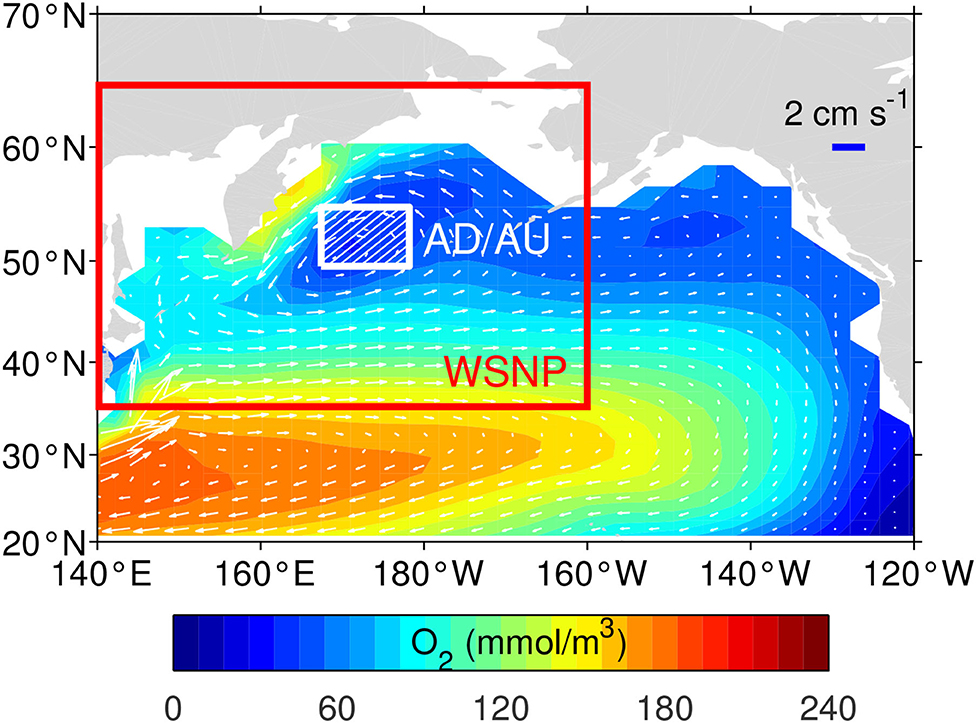
Figure 1. Zoomed in view of the Subarctic North Pacific embedded with year 2020 model-simulated oxygen concentration (color) and velocity vectors (arrows) at a depth of 457.5 m (i.e., model level 5). The red box (140 E–160 W, 30–65 N) defines the Western Subarctic North Pacific (WSNP); the white shadow area (167–179 E, 49–55 N) highlights the location where AD and AU pipes are installed.

AD and AU are simulated in the core region of the WSNP (~440,000 km², the shadow area in Figure 1) for the period of 2020–2100. Since engineered pipes are small and difficult to be resolved in the current coarse-resolution model, they are parameterized as suggested by Feng et al. (2020) and Oschlies et al. (2010). In AD case, dissolved ocean tracers are adiabatically transferred from a model grid box containing the pipe's upper end to another model grid box containing the lower end of the pipe at a constant velocity w (< 0). Therefore, we introduce the tracer source terms of wC_t and −wC_t at the designated surface and deeper grid boxes, respectively, and C_t is the tracer concentration. To conserve the volume, water released from the lower end of the pipe is assumed to drive a uniform upward flow to the upper end of the pipe, i.e., a constant compensating velocity −w across all intermediate levels. For simulating AU, we make the sign of w opposite to that of AD since the two engineering schemes operate in opposite directions.

In the standard AD and AU simulations, pipe extensions are from a near-surface depth of 17.5 m (model level 1) to an intermediate depth of 457.5 m (model level 5); the pipe length is thus 440 m. Provided that the pumping capacity of a technologically feasible pipe exploiting energy from waves or tides varies from 0.3 to 1 m³/s (Antonini et al., 2015; Xiao et al., 2018), the required pipe number is 0.2–0.66 million to achieve a total downwelling flow rate of 0.20 Sv. This corresponds to a transfer velocity of |w|=4 cm/day in the deployment site (~440,000 km²), with 0.5–1.5 pipes installed per kilometer square. To study the impact of engineering parameters, we also carried out six additional AD simulations with different pipe lengths (i.e., 160, 285, and 625 m) and different transfer velocities (i.e., 2, 6, and 8 cm/day). In these simulations, only the value of the sensitivity parameter is altered, and other parameters are kept at their values in the standard AD case.

3. Results and Discussion

3.1. Model Validation

Simulated global pattern of oxygen, e.g., at a model level of 457.5 m, achieves a good fit to the observation derived from the WOA 2018 dataset (Garcia et al., 2019). Because observation data are collected on or after 1960, model outputs are averaged between 1960 and 2020 for comparison. The model well captures the feature of low-oxygen (O₂ below 60 mmol/m³) water in the global ocean (Figure 2a). This low-oxygen water is mainly distributed in the tropical oceans and the subpolar North Pacific. Its boundaries simulated by the model are in good agreement with observations (Figure 2b). Oxygen level are generally higher in the polar regions, because cold wintertime surface ocean temperature increases oxygen solubility and enhanced wind stress intensifies ventilation. For the region above 60° N, model-simulated 457.5 m oxygen ranges from 220 to 320 mmol/m³, in agreement with the observation of 180–360 mmol/m³.

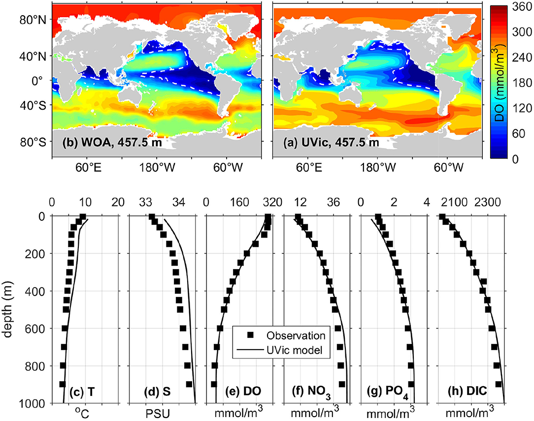
Figure 2. Model-data comparison: (a) Simulated and (b) observed global oxygen pattern at a depth of 457.5 m; (c–h) simulated (lines) and observed (scatter) basin averaged profiles of key model tracers within the WSNP (T, temperature; S, salinity; DO, dissolved oxygen; NO₃, nitrate; PO₄, phosphate; DIC, dissolved inorganic carbon). All the observations are derived from the World Ocean Atlas 2018 (WOA 2018) (Garcia et al., 2019), expect for the DIC profile derived from GLODAPv2.2020 (Olsen et al., 2019, 2020). The observational data are collected on or after 1960, and model outputs for the historical comparisons are averaged between 1960 and 2020. In (a,b), white dash lines delineate the contour of low-oxygen areas (O₂ <60 mmol/m³).

Focussing our model-data comparison to the WSNP, Figures 2c–h indicates good matches between simulated and observed basin averaged profiles of key model tracers. Observations of temperature, salinity, oxygen, nitrate, and phosphate are derived from WOA 2018 (Garcia et al., 2019), and dissolved inorganic carbon is derived from GLODAPv2.2020 (Olsen et al., 2019, 2020). 1960–2020 period is still used for averaging model outputs. For temperature and salinity, the model overestimates them by <2°C and 0.4 PSU, respectively, with major misfits occurring above 600 m (Figures 2c,d). These misfits, however, largely cancel each other in their impact on water density, for which the model presents almost correct stratified conditions. Other tracers have relatively small differences when comparing the model and data (Figures 2e–h).

Regarding the temporal variability, the scarcity of observational data leads us to only focus on changes in temperature, salinity, and oxygen within the WSNP. In the historical simulation between 1765 and 2000, the variations of tracer quantities can be calculated at any depth through interpolation. From 1950 to 2000, our model indicates oxygen in the 200–400 m range of the WSNP decreasing at a mean rate of 18 mmol/m³/yr, within the observed range of 15–21 mmol/m³/yr (Keeling et al., 2010). Meanwhile, the model indicates warming (0.62 °C/century) in the 50–900 m range of the Western Subpolar Gyre (48–60°N, 160–170°E), stronger than the observation (0.31 ± 0.28°C/century); and freshening (−0.06 PSU/century) in the 90–100 m deep water in Bering Sea (50–60° N, 180–170° W), weaker than the observation (−0.31 ± 0.22 PSU/century) (Andreev and Watanabe, 2002). These inconsistencies for temperature and salinity are likely due to the multidecadal variability of the global wind forcing that resulted from the strengthening of Antarctic Circumpolar Current and Pacific Decadal Oscillation not being well resolved in the model (Schmittner et al., 2008). Fortunately, our model still correctly presents the observed trend in stratification. The intensity of stratification in the WSNP, measured by the density difference between surface (0–240 m) and subsurface (240–960 m) water, are generally 6% higher in the year 2000 compared with 1950, consistent with the increasing trend in stratification suggested by Andreev and Watanabe (2002). Our simulations present a good correlation between the increase in the stratification intensity and subsurface oxygen loss in the WSNP in their spatial patterns, also consistent with Andreev and Watanabe (2002).

3.2. General Oxygen Pattern

With no engineering, climate change decreases oxygen content in the WSNP's mid-depth water throughout the century. The climate impact here is illustrated by the field anomalies, the year 2050 and 2100 minus 2020, of oxygen content at a model level of 457.5 m in the reference simulation (Figures 3a,d). Within the WSNP region (red box in Figure 3a), oxygen at 457.5 m depth decreases by 10–40 mmol/m³ in 2050 and 30–100 mmol/m³ in 2100. Increasing stratification could be a leading factor driving these oxygen declines as previously found in the 1950–2000 simulation. From 2020 to 2100, stratification gets stronger as a result of surface and subsurface warming of about 3 and 1°C, respectively; the salinity change has a minor impact on the stratification. Another reason for the decreased oxygen could be warming-induced accelerated aerobic remineralization that consumes more oxygen in the subsurface water (our model suggests a 13% increase in remineralization rate for 1°C temperature rise). However, this possibility is rejected by simulated reduced aerobic remineralization in the WSNP's intermediate water (Figures 3g,j). Such reduction results from intensified stratification, which inhibits nutrient supply to the sunlit layer and subsequent carbon export across the pycnocline (Sarmiento et al., 1998; Jang et al., 2011). The simulated most rapid oxygen decline occurs in the shelf water of the WSNP (Figures 3a,d). Andreev and Watanabe (2002) has indicated that in the Bering Sea where the shelf water originally forms, winter ventilation for oxygen supply is weakened by the freshening of surface seawater because of reduced ice formation and altered atmospheric forcing. This remote effect in the Bering Sea ultimately drives the rapidly decreasing oxygen presented in the shelf water. Our model might agree with Andreev's finding, by showing up to 1 PSU salinity decrease in surface water of the Bering Sea and its adjacent shelf region in 2100, greater than elsewhere in the WSNP.

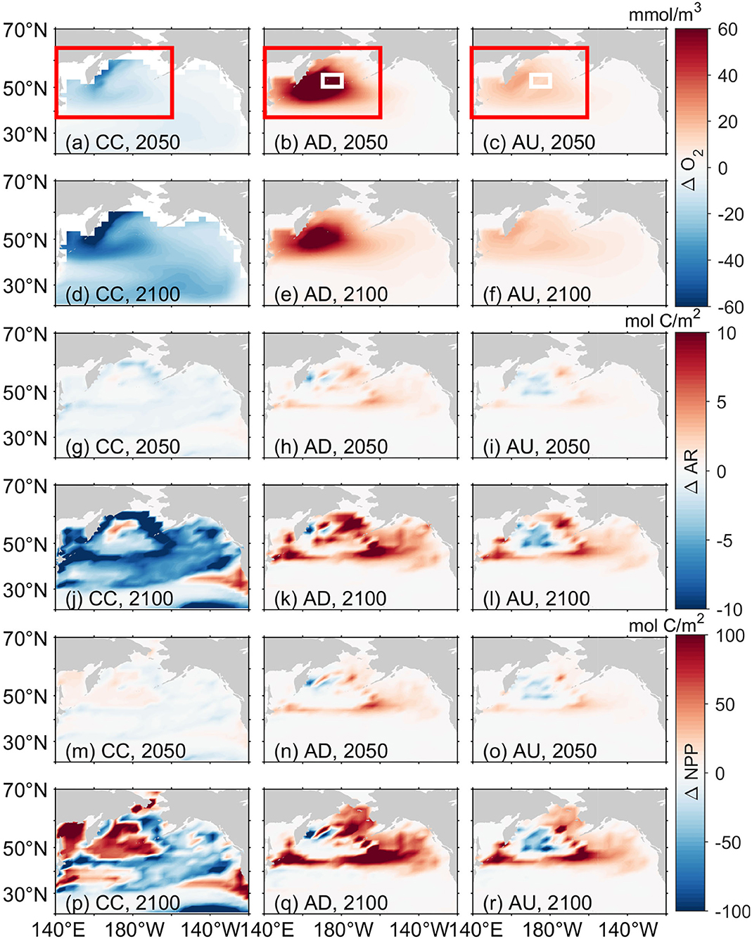
Figure 3. Field anomalies caused by climate change (CC, left), artificial downwelling (AD, middle), and artificial upwelling (AU, right) at year 2050 and 2100: (a–f) oceanic oxygen at 457.5 m (i.e., model level 5); (g–l) cumulative aerobic remineralization (240–960 m); (m–r) cumulative net primary production (0–240 m). Cumulative time periods are from year 2020 to 2050 or 2100. The impacts of climate change here and in other figures are calculated as differences from year 2020 background field; the impacts of AD and AU here and in other figures are calculated as the differences of their standard simulations relative to the reference simulation at the same model year (Red box: WSNP; white box: locations of pipe installation).

AD and AU both increase oxygen in the intermediate layer of the WSNP. Here, we calculate the anomalies of two standard simulations relative to the reference simulation at 457.5 m depth (Figures 3b–f); the depth selected is the position of the lower ends of the pipes. In the standard cases, oxygen is up to 90 (AD) and 21 (AU) mmol/m³ higher in the year 2100 than if the engineering has not been implemented. Because climate change decreases oxygen by up to 40 mmol/m³ with respect to the year 2020 data (Figure 3d), running AD from 2020 to 2100 prevents mid-depth oxygen decline in the WSNP while running AU suppresses it.

Figure 4 further describes basin averaged profiles of the oxygen anomalies, AD or AU minus the reference run, after 10, 30, and 80 years of pipe installation. When AD is implemented, oxygen is improved in deep water, with the largest improvement occurring at 457.5 m where surface oxygen-rich water is released. The released water drives the upward motion of deep water, reducing oxygen in the upper ocean. Near the surface, oxygen is almost the same as in the non-engineered case, as a result of a tradeoff between compensatory upwelling of deep low-oxygen and enhanced air-sea oxygen flux during AD (Feng et al., 2020). Turning to the AU case, water experiences a more evenly distributed oxygen improvement. For depth greater than 240 m, AU improves oxygen less effectively than AD, with the largest improvement, only about half of that in AD, occurring at 300 m. Unexpectedly, while AU brings deep low-oxygen water to the ocean surface, the upper ocean experiences an increase in oxygen. Probably, deep low-oxygen water exposed to the air immediately reaches saturated status. AU then increases oxygen below the ocean surface via generating a compensatory downward flow outside of the pipe. The profiles of anomalies at different years imply that after 2050, the oxygen improvement in the 100–600 m range is attenuated in the AD case but slightly strengthened in the AU case. The mechanism controlling the temporal variations of oxygen improvement will be discussed in the next section.

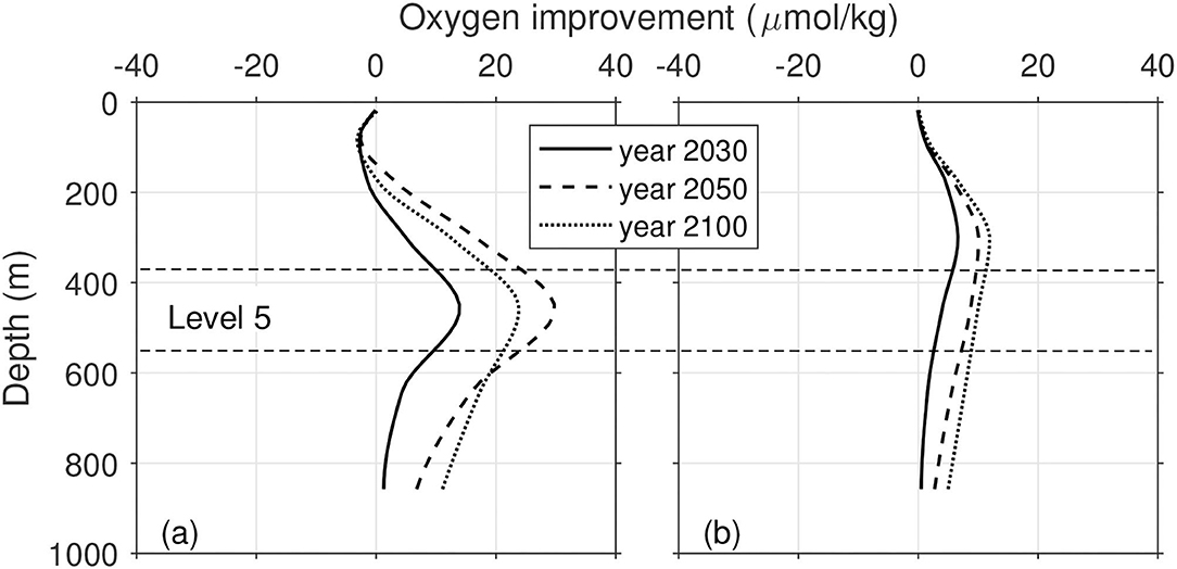
Figure 4. Basin averaged vertical profiles of oxygen anomaly within the WSNP relative to the reference run after 10 (solid), 30 (dash), and 80 (dotted) years of pipe operating: (a) standard AD; (b) standard AU.

Notably, net primary production (NPP) responds differently inside and outside of the core region of the WSNP, i.e., the Western Subpolar Gyre, over the century (Figures 3m,p). NPP consists of new PP and regenerated PP. Warming-induced stratification tends to prevent nutrient exchange across the pycnocline, reducing new PP in the upper ocean (Sarmiento et al., 1998; Jang et al., 2011). On the other hand, our model with a simple parameterization of the microbial loop suggests faster remineralization and more regenerated PP in the euphotic layer under warmer conditions (Taucher and Oschlies, 2011). The trade-off between these two effects is thus able to explain cumulative changes in NPP. Within the core region of the WSNP, surface nutrients are sufficient in the year 2100 (N: 13–15 mmol/L; P: ~1 mmol/L), indicating that phytoplankton growth is not limited by macro-nutrients and insensitive to additional variations of nutrient supply from below the pycnocline. In this case, increased regenerated PP rather than new PP accounts for the enhanced NPP. Outside of that region, surface nutrients are thoroughly utilized and approximate zero concentration. Limited nutrient exchange associated with warming thus explains the decreased net primary production there. Nitrogen fixation and loss are neglected for the above estimates. Both our simulations and others' studies (e.g., Wang et al., 2019) indicate inactive nitrogen fixation within the WSNP, a place where diazotrophs do not survive with poor iron supply from dust deposition and low temperature of surface water. Meanwhile, nitrogen loss associated with denitrification never happens since oxygen within the WSNP is far from reaching a suboxic state. For the above reasons, only the ordinary phytoplankton class is considered to participate in biogeochemical cycling.

3.3. Mechanism

To reflect the temporal variations of oxygen improvement, Figure 5 plots the time series of the time derivatives (red solid lines) of oxygen inventory anomaly, relative to the non-engineered case, within the WSNP at the fifth model layer (i.e., 380–550 m highlighted in Figure 4). Variations of the time derivative term imply that oxygen improvement is completed within the first 40 years of pipe installation in both engineering cases, and after that, weakly reduced in the AD case and increased in the AU case.

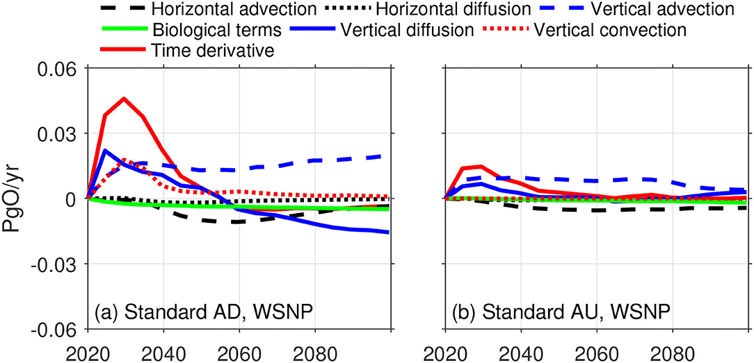
Figure 5. Time series of (a) AD and (b) AU-induced anomalies, relative to the reference run, of oxygen budget terms integrated within the WSNP at the fifth model layer (i.e., 380–550 m highlighted in Figure 4). Note that vertical advection terms here and in the main text include direct and indirect pumping fluxes.

Different time derivatives of oxygen inventory anomaly between the AD and AU case are due to that two engineering schemes have different mechanisms improving oxygen at the target depth via multiple physical processes. This can be inferred from other time series, also shown in Figure 5, of induced anomalies of oxygen budget terms relative to the non-engineered case, integrated within the WSNP at the fifth model layer. The anomalies of biological terms are rather small compared to those of physical terms, suggesting a weak impact of biological activities on the engineered oxygenation. When AD is initially implemented before 2030 (Figure 5a), discharge of surface water at the lower end of the pipes increases vertical advection by locally increasing oxygen concentration. Meanwhile, less dense surface water causes buoyancy-driven pycnocline mixing, explaining the enhanced convection. The increased vertical diffusion is likely due to increased pycnocline mixing that results in less stratified conditions and thus a larger vertical diffusion coefficient (at this point, the vertical gradient of oxygen remains positive). These physical processes contribute to major oxygenation during the first 10 years of AD implementation. After 2030, the enhancement in the convection becomes increasingly weak as engineering-induced mixing causes more and more uniform density profiles. The vertical diffusion enhancement is also attenuated for a decreasing vertical gradient of oxygen. This together with increasingly strong horizontal advection of oxygen toward the outside of the WSNP results in oxygen improvement rapidly declined to approximate zero in 2060. For the AU case, oxygen is indirectly improved by the compensatory downwelling, which, however, takes much longer than pipe-inside downwelling to bring surface oxygen-rich water to the target depth and thus causes less increased vertical advection. In addition, cold water extracted from the deep ocean tends to sink down after discharge due to the negative buoyancy, but this only enhances shallow mixing instead of pycnocline mixing, resulting in no enhancement in convection and weakly increased vertical diffusion. Consequently, AD improves oxygen more effectively than AU at the target depth via stronger vertical advection and extra enhancement in pycnocline mixing. A similar discrepancy between AD and AU can be seen from sensitivity simulations using different pipe lengths (not shown). Overall, AD outperforms AU in mid-depth oxygenation. The mentioned strengthened pycnocline mixing during AD has been suggested by some nearfield studies (Stigebrandt et al., 2015; Xiao et al., 2019). In their field experiment in By Fjord, Stigebrandt et al. (2015) found that below-pycnocline mixing is intensified by the plume-like compensatory upwelling at a scale of several kilometers.

In Figure 5a, the negative anomaly of the vertical diffusion after 2060 is almost confined to the subsurface (240–980 m) layer so that for the entire subsurface layer vertical advection of oxygen is instead primarily balanced by the horizontal advection, similar to the AU situation. This implies that most of the oxygen AD and AU add to the subsurface layer of the WSNP is horizontally advected out during the new equilibrium stage (i.e., 2060–2100).

While our model suggests a weak biological impact on the engineered oxygenation, it seems to be inconsistent with Feng et al. (2020)'s finding of strongly increased aerobic remineralization after AD or AU pipes are deployed, which consumes a large amount of mid-depth oxygen. Our simulations show weak enhancement in aerobic remineralization whereas large increase in primary production during the implementation of the engineering. For two standard engineering simulations, nutrients that AD or AU brings to the ocean surface stimulate NPP outside of the core region of the WSNP where macro-nutrients are a limiting factor for phytoplankton growth (Figures 3n–r). AU shows a generally less increase in primary production as compared with AD. An explanation is less nutrient supply to the surface ocean in the AU case where pycnocline mixing is not as strong as AD due to the lack of convection as well as less vertical diffusion. In both engineering cases, the cumulative increases in NPP since 2020 both amount to 100 mol C/m² by the year 2100 (Figures 3q,r). In contrast, cumulative changes in the aerobic remineralization (240–960 m) are much smaller than those in the net primary production, while the two show a close relationship. In the AD scenario (Figures 3h,k), about 10 mol C/m² increase in cumulative remineralization is seen outside of the upwelling region by 2100. The enhancement thus accounts for 10% of net primary production increase. Our model suggests that 22% increase of net primary production participates in nutrient recycling (including microbial process) in the shallow water (above 240 m), 50% goes into the zooplankton community, and the remaining part is in the form of detritus. For the mentioned ~10 mol C/m² enhancement of cumulative remineralization in 240–980 m water, a cumulative respiratory oxygen demand would be about 13 mmol/m³. This explains attenuation in the oxygenation in the AD case when comparing Figures 3b,e. Brewer and Peltzer (2017) has suggested that many of current biogeochemical models including ours underestimate the warming sensitivity of aerobic remineralization. However, even full decomposition of the increased primary production within this century, i.e., ~100 mol C/m², consumes oxygen by up to 30 mmol/m³, far less than the addition induced by AD. In the AU scenario (Figures 3i,l), less cumulative remineralization is related to less NPP. As a result, there is a reduction and an increase in remineralization inside and outside of the upwelling region, respectively, causing no change in the basin-averaged anomaly of biological terms (Figure 5b). The weak impact of aerobic remineralization is consistently suggested by our sensitivity experiments of AD with different pipe lengths and downwelling rates (not shown).

The resulting oxygenation has benefits such as reducing the volume of low-oxygen water. In the standard AD and AU experiments, oxygen-deficient water, defined as oxygen content below 60 mmol/m³, shows an expansion of 4 and 24%, respectively, by 2100, both less than the 37% expansion caused by climate change. Increasing the downwelling rate yields less expansion or even compression of oxygen-deficient water. For the downwelling rate of 2, 4 (standard AD), 6 and 8 cm/day, the expansion would be 29, 4, −8, and −16%, respectively. Thus, AD with a downwelling rate of 4~6 cm/day could prevent oxygen-deficit water from expanding within this century. This requires a total downwelling rate of 0.2~0.3 Sv in the deployment site, namely 1–1.5 million pipes for an averaged pipe flow rate of 0.2 m³/s. The impact of pipe lengths is also studied. AD simulations using the pipe length of 160, 285, 440, and 625 m suggest oxygen-deficit water increased by 25, 11, 4, and 24%, respectively. Hypoxic water growing more slowly with increasing pipe length except for 625 m simulation is a consequence of longer pipes closer to the core region of low-oxygen water, which is estimated deeper than 400 m. Compared to 440 m pipe, 625 m pipe instead suggests a greater expansion of oxygen-deficit water, likely due to less pycnocline mixing enhancement with deeper discharge (Xiao et al., 2019). The optimal discharging depth thus is where oxygen content reaches sufficiently low to necessitate oxygenation and as close as possible to the pycnocline depth.

3.4. Mitigating Deoxygenation

AD and AU both effectively mitigate deoxygenation in the WSNP. In three base runs, the oxygen inventory, calculated within the WSNP for the water column shallower than 1,000 m, decreases from 43.9 Pg O in 2020 by 8.4 (the reference), 4.2 (standard AD), and 5.9 Pg O (standard AU) in 2100. Thus, AD and AU increase it relative to the reference case by 4.2 and 2.5 Pg O, respectively (Figure 6a). Close examinations suggest that air-sea exchange and horizontal advection have a dominant impact on the WSNP's oxygen inventory increase caused by AD and AU. The impact of biological activities is secondary. Contributions of other terms are negligible. In the AD case, for example, enhanced air-sea exchange leads to an oxygen inventory increase by 9.5 Pg O, and 6.4 Pg O of it is horizontally advected out. Meanwhile, biological activities only increase the oxygen inventory by 1.1 Pg O, with a production of 1.6 Pg O via photosynthesis and a consumption of 0.5 Pg O via remineralization. The ultimate increase is 4.2 Pg O, 40% greater than in the AU case where the contribution of the aforementioned terms has a similar order. Therefore, in both AD and AU cases, the WSNP's oxygen inventory is increased by enhanced the air-sea downward flux of oxygen, yet more than half of the increase caused by air-sea exchange enters into the outside of the WSNP by horizontal advection.

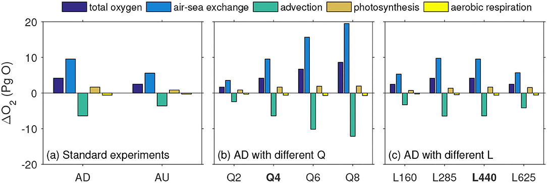
Figure 6. Cumulative changes in the WSNP's oxygen inventory in (a) the standard AD and AU simulations, (b) AD simulations with a downwelling rate of 2, 4, 6, 8 cm/day, and (c) AD simulations with a pipe length of 160, 285, 440, and 625 m. For each model run, the cumulative change in the oxygen inventory is split into different components (shown in the legend). All the components are integrated above 960 m within the WSNP region from year 2020 to 2100.

Furthermore, Figures 7a,b suggest the leading role of air-sea exchange and horizontal advection in modulating the oxygen inventory. Here, the time series of the induced anomalies of oxygen budget terms relative to the non-engineered case are integrated within the WSNP for the water column shallower than 1,000 m. The downward air-sea fluxes of oxygen in the standard AD and AU case respond rapidly at the beginning, increasing to 0.11 and 0.05 Pg O/year higher than the non-engineered case in 2030, respectively. Thereafter, they both gradually decline to become stable at 0.02 Pg O/year higher than the non-engineered case toward the end of the simulations. The increased downward fluxes over time indicate the WSNP's ability to uptake more oxygen from the atmosphere in the presence of engineering. This ability simultaneously is undermined by the increasingly strong advection of oxygen toward the outside of the WSNP. As a result, the rates of oxygen inventory increase (i.e., the time derivative anomaly) decline in both AD and AU cases after 2030. Two engineering schemes no longer mitigatie deoxygenation in the WSNP as the rate of the oxygen inventory increase approaches to zero.

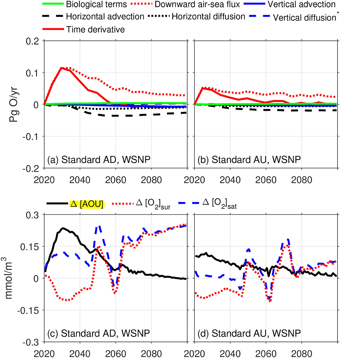
Figure 7. Time series of (a) AD and (b) AU-induced anomalies of oxygen budget terms integrated within the 0–960 m range of the WSNP. The time derivative (red solid) is the sum of the biological terms (green solid), air-sea exchange (red dotted), water mass advection (blue solid for vertical; black dash for horizontal) and diffusion (blue dash for vertical; black dotted for horizontal). To understand air-sea oxygen change, we also give (c) AD and (d) AU-induced temporal variations of apparent oxygen utilization (AOU) at the ocean surface (black solid lines). AOU = [O2]_sat-[O2]_sur, where [O2]_sat is the oxygen saturation (blue dash) and [O2]_sur is the actual oxygen content (red dotted).

The underlying mechanism of AD and AU increasing the air-sea oxygen flux is explored by their induced anomalies of apparent oxygen utilization (hereafter AOU) at the surface (Figures 7c,d). When AD or AU is initially operated, deep, cold, and low-oxygen water is indirectly or directly upwelled to the upper ocean. Surface oxygen (spatially averaged in the WSNP) then slightly decreases with respect to the non-engineered case, and oxygen saturation increases due to the cooling effect. AOU, calculated by the oxygen saturation minus the actual oxygen content, thus increases at the surface, resulting in an enhanced air-sea oxygen flux (f_o2 = k_o2 [AOU] according to Garcia and Keeling, 2001). After 2060, as deep already oxygenated water comes up to shallow depths, surface oxygen content increases and approaches the oxygen saturation, causing AOU and the flux no longer to increase. The oxygen inventory then ceases to grow.

AD tends to generate larger air-sea oxygen flux than AU and thus is more capable of adding oxygen to the WSNP (Figures 7a,b). Two engineering schemes induce similar anomalies of surface oxygen content but quite different anomalies of oxygen saturation (Figures 7c,d). Such discrepancy is likely because local natural upwelling interacts with the near-field compensatory flows in the presence of engineering. During AD, the compensatory upward flow of 4 cm/day together with the local upwelling causes a more intense cooling effect compared to the non-engineered case, resulting in the positive anomaly of oxygen saturation (Figure 7c). During AU, the compensatory downward flow of 4 cm/day instead significantly undermines the surface cooling brought by the local upwelling of about 8 cm/day, which counterbalances enhanced surface cooling due to upwelling inside pipes to give almost zero anomaly of oxygen saturation from the non-engineered case (Figure 7d).

Engineering strategies have a large impact on the oxygenation effect (Figures 6b,c). The oxygen inventory increases almost linearly with increasing downwelling rate, for that a downwelling rate of 2, 4 (standard AD), 6, and 8 cm/day yields a inventory increase of 1.7, 4.2 (standard AD), 6.7, and 8.6 Pg O, respectively. To combat the WSNP's deoxygenation under climate change, which leads to the 8.4 Pg O decline by 2100, about 8 cm/day downwelling rate needs to be achieved in the deployment site (i.e., a total flow rate of 0.4 Sv). In that regard, the required number of pipes with a pumping capacity of 0.2 m³/s is 2,000,000. The increase in the oxygen inventory also varies with pipe lengths. A pipe length of 160, 285, 440, and 625 m gives a inventory increase of 2.5, 4.2, 4.2 (standard AD), and 2.5 Pg O, respectively. The oxygen inventory initially increased with increasing pipe length is due to that with the upwelling of deeper, colder, and more hypoxic water, associated enhanced air-sea oxygen flux allows the ocean to dissolve more atmospheric oxygen. However, when surface water is discharged below the pycnocline, the variability of both temperature and oxygen content is not as strong as in shallow water. Instead, induced pycnocline mixing decreases with greater discharging depth, thus likely causing the decline in the oxygen inventory when transiting the pipe length from 440 to 625 m.

3.5. Environmental Side Effects

AD and AU regionally affect the local carbon cycle. The carbon export flux across the air-sea interface is changed due to the engineering. In the reference simulation, the WSNP tends to absorb atmospheric carbon dioxide under climate change, indicated by a generally increased air-sea carbon flux (toward the ocean) in 2100 relative to 2020 (Figure 8a). However, AD or AU decreases the downward carbon flux within and nearby the deployment region, causing a “carbon source” effect. This is likely due to the indirect or direct upwelling of high dissolved inorganic carbon (hereafter DIC) water from the deep ocean (Figures 8b,c). The engineering influence is negligibly small compared with that of elevated atmospheric CO₂, since the basin-averaged downward DIC flux increases by 37, 36, and 35% in 2100 relative to 2020 under the reference, AD, and AU scenarios, respectively. The sequestration efficiency of the biological carbon pump (BCP) is also evaluated. This quantity in the model is calculated as the ratio of the carbon export at the model level of 980 m to that of 130 m. The sequestration efficiency will decrease from 14.5% in 2020 to 12.9, 13.0, and 13.0% in 2100, respectively. Marginally elevated sequestration efficiency in two engineering cases may result from surface cooling effect that deaccelerates respiration in shallow water and increases subsequent carbon export to depth.

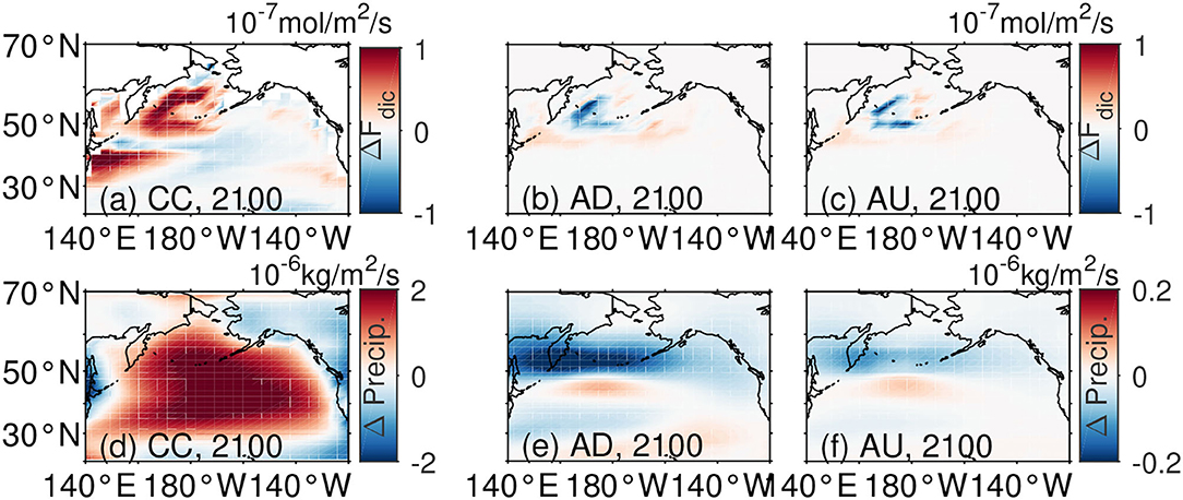
Figure 8. Field anomalies of (a–c) dissolved inorganic carbon flux and (d–f) precipitation flux in the year 2100 with respect to 2020, caused by climate change (CC, left), artificial downwelling (AD, middle), and artificial upwelling (AU, right).

Other side effects related to AD and AU include regionally decreased precipitation and ocean pH. As a result of global warming, more intense evaporation spreads over the North Pacific, increasing the precipitation rate by over 2 × 10⁻⁶ kg/m²/s in 2100 relative to 2020 (Figure 8d). AD and AU instead reduce the precipitation rate via surface cooling effect, by up to 2 × 10⁻⁷ and 0.5 × 10⁻⁷ kg/m²/s, respectively, in 2100 (Figures 8e,f). Less reduction in AD with respect to AU is because AD produces stronger surface cooling through a combination of engineering compensatory and natural upwelling in the WSNP, as already discussed in section 3.4. The response of precipitation to the engineering is much less evident than that to climate change. Regarding the ocean acidification, surface ocean pH within the WSNP will slightly decrease by <0.03 by the year 2100 because more acid deep water is upwelled. Likewise, such a pH decrease is much less than that (~0.4) caused by the climate change.

Globally, two engineering schemes slightly reduce the averaged surface air temperature by <0.02°C throughout the century. The major temperature decline occurs in the northern hemisphere. Deep and cold ocean water upwelled directly by AU or indirectly by AD is responsible for such a cooling effect. In 2100, there are also 0.18 and 0.26 Gt C higher global total atmosphere carbon in AD and AU compared with the reference simulation, both corresponding to <1 ppm increase in global annual atmospheric CO₂. As previously suggested, the indirect or direct upwelling leads to more carbon uptake from the air via stimulating primary production, yet it brings deep water rich in DIC to the surface ocean. The net result is a slight carbon export toward the air. The results shown here suggest a weak influence that AD and AU impose on the global climate system.

4. Summary

While previous modeling studies consistently project continued deoxygenation in the WSNP over this century, this study focuses on two short-term remediation solutions, i.e., AD and AU, both aiming to improve the oxygen in deep water through pipes. Our simulations suggest that AD substantially enriches the WSNP's mid-depth oxygen via directly releasing surface oxygen-rich water from the lower ends of the pipes, and AU more weakly does so via nearfield compensatory downward flow outside the pipes. With no engineering intervention, there will be a 33% expansion of hypoxic water in the WSNP by 2100, potentially posing a threat to the fisheries and ecosystem functioning. Implementing AD and AU instead reduces the 33% expansion to 5 and 27%, respectively, provided with one pipe installed per square kilometer (the deployment site is 440,000 km²), a pipe flow rate of 0.46 m³/s, and pipe extension from near the surface to 457.5 m depth. The results thus confirm the efficacy of AD and AU in improving mid-depth oxygen in the WSNP.

Different potentials of AD and AU to improve mid-depth oxygen are a consequence of how they redistribute oxygen vertically via different physical processes. During AD, surface oxygen-rich water is discharged at the lower ends of the pipes and then rises due to buoyancy. This enhances not only the vertical advection of oxygen toward the target depth but also pycnocline mixing, both facilitating downward oxygen supply. Compared to AD, AU instead creates less vertical advection through the compensatory downwelling outside of the pipes. Meanwhile, the downwelling of deep water discharged increases shallow mixing rather than pycnocline mixing. For these reasons, AD outperforms AU at improving mid-depth oxygen. Biological activities only have a secondary impact on the engineered oxygenation due to a small fraction of fertilization-induced primary production enhancement decomposed in mid-depth water.

AD and AU could also mitigate deoxygenation in the WSNP as they increase its oxygen inventory. The underlying mechanism of oxygen addition is enhanced air-sea oxygen exchange. AD increases apparent oxygen utilization (AOU) at the surface ocean by nearfield compensatory upwelling of cold and oxygen-deficient water, thus increasing the tendency of the WSNP to absorb oxygen from the air; AU similarly does so by direct upwelling inside pipes. However, AD increases the oxygen inventory more than AU, which can be explained by stronger surface cooling brought by AD with compensatory upwelling intensifying local natural upwelling whereas during AU the compensatory downwelling undermines it.

Environmental side effects are also studied. While both engineering schemes weakly influence the global climate system, they regionally cause CO2 outgassing, precipitation reduction, and ocean acidification. Fortunately, these consequences are nowhere near as pronounced as those caused by rapid climate change.

In order to obtain the most considerable improvement of oxygen in the WSNP, the optimal strategy is to implement AD by discharging water at the depth where oxygen content reaches sufficiently low to necessitate oxygenation and as close as possible to the pycnocline depth. If the discharging depth is too far away from the pycnocline depth, AD cannot sufficiently increase pycnocline mixing. Meanwhile, increasing the number of pipes or the pipe flow rate helps to achieve more intense oxygenation. Nevertheless, AD and AU are only effective within the first 40 years of operation, whether in terms of oxygen content improvement, low-oxygen water reduction, or oxygen inventory increase. Oxygen barely changes after the WSNP reaches a new equilibrium state in a perturbed world.

Results revealed by our simulations indicate that subpolar gyre regions such as the WSNP could be an ideal site to deploy AD or AU pipes for mitigating deoxygenation. With the same model, Feng et al. (2020) has found that these geoengineering approaches are relatively ineffective in restoring oxygen in the tropical oxygen-deficit zones. Since all these simulations parameterized the engineering as a uniform translocation between two model layers, they may not correctly present AD and AU's nearfield dynamics, resulting in more uncertainties about engineering consequences. Efforts are required to develop fine-resolution regional models for AD and AU.

Data Availability Statement

The observation data used for this study is available through Garcia et al. (2019) and Olsen et al. (2019, 2020). Model results used to create all figures in the paper, as well as the modified UVic code to simulate AD and AU, are available on Zenodo repository (http://doi.org/10.5281/zenodo.5201702).

Author Contributions

CX: conceptualization, original drafting, and programming and visualization. WF: conceptualization, review, and editing. YC, YZ, KT, and NJ: resources, review, and editing. All authors contributed to the article and approved the submitted version.

Funding

This research was supported by the National Natural Science Funds of China (No. 41976199), National Key Research and Development Program of China (No. 2019YFD0901320), Strategic Priority Research Program of the Chinese Academy of Sciences (XDA23050303), and National Key Research and Development Program of China (No. 2016YFA0601400). This study is a contribution to the international IMBeR project.

Conflict of Interest

The authors declare that the research was conducted in the absence of any commercial or financial relationships that could be construed as a potential conflict of interest.

Publisher's Note

All claims expressed in this article are solely those of the authors and do not necessarily represent those of their affiliated organizations, or those of the publisher, the editors and the reviewers. Any product that may be evaluated in this article, or claim that may be made by its manufacturer, is not guaranteed or endorsed by the publisher.

Acknowledgments

We thank reviewers for helpful comments on the manuscript and appreciate Long Cao from Zhejiang University for his technical support on UVic model setup as well as Mike Eby from the UVic model support team.

References

Andreev, A., and Watanabe, S. (2002). Temporal changes in dissolved oxygen of the intermediate water in the subarctic north pacific. Geophys. Res. Lett. 29, 25–31. doi: 10.1029/2002GL015021
Antonini, A., Lamberti, A., and Archetti, R. (2015). Oxyflux, an innovative wave-driven device for the oxygenation of deep layers in coastal areas: a physical investigation. Coast. Eng. 104, 54–68. doi: 10.1016/j.coastaleng.2015.07.005
Beamish, R., Leask, K., Ivanov, O., Balanov, A., Orlov, A., and Sinclair, B. (1999). The ecology, distribution, and abundance of midwater fishes of the subarctic pacific gyres. Prog. Oceanogr. 43, 399–442. doi: 10.1016/S0079-6611(99)00017-8
Breitburg, D., Levin, L. A., Oschlies, A., Grégoire, M., Chavez, F. P., Conley, D. J., et al. (2018). Declining oxygen in the global ocean and coastal waters. Science 359:6371. doi: 10.1126/science.aam7240
Brewer, P. G., and Peltzer, E. T. (2017). Depth perception: the need to report ocean biogeochemical rates as functions of temperature, not depth. Philos. Trans. R. Soc. A Math. Phys. Eng. Sci. 375:20160319. doi: 10.1098/rsta.2016.0319
Diaz, R. J., and Rosenberg, R. (2008). Spreading dead zones and consequences for marine ecosystems. Science 321, 926–929. doi: 10.1126/science.1156401
Eby, M., Weaver, A. J., Alexander, K., Zickfeld, K., Abe-Ouchi, A., Cimatoribus, A., et al. (2013). Historical and idealized climate model experiments: an intercomparison of earth system models of intermediate complexity. Clim. Past 9, 1111–1140. doi: 10.5194/cp-9-1111-2013
Feng, E. Y., Su, B., and Oschlies, A. (2020). Geoengineered ocean vertical water exchange can accelerate global deoxygenation. Geophys. Res. Lett. 47:e2020GL088263. doi: 10.1029/2020GL088263
Garcia, H. E, Weathers, K. W., Paver, C. R., Smolyar, I., Boyer, T. P., Locarnini, R. A., et al. (2019). World Ocean Atlas 2018, Volume 3: Dissolved Oxygen, Apparent Oxygen Utilization, and Dissolved Oxygen Saturation. NOAA Atlas NESDIS 83, 38.
Garcia, H. E., and Keeling, R. F. (2001). On the global oxygen anomaly and air-sea flux. J. Geophys. Res. 106, 31155–31166. doi: 10.1029/1999JC000200
Jang, C. J., Park, J., Park, T., and Yoo, S. (2011). Response of the ocean mixed layer depth to global warming and its impact on primary production: a case for the North Pacific ocean. ICES J. Mar. Sci. 68, 996–1007. doi: 10.1093/icesjms/fsr064
Keeling, R. F., Körtzinger, A., and Gruber, N. (2010). Ocean deoxygenation in a warming world. Annu. Rev. Mar. Sci. 2, 199–229. doi: 10.1146/annurev.marine.010908.163855
Keller, D., Oschlies, A., and Eby, M. (2012). A new marine ecosystem model for the University of Victoria earth system climate model. Geosci. Model Dev. 5, 1195–1220. doi: 10.5194/gmd-5-1195-2012
Keller, D. P., Feng, E. Y., and Oschlies, A. (2014). Potential climate engineering effectiveness and side effects during a high carbon dioxide-emission scenario. Nat. Commun. 5, 1–11. doi: 10.1038/ncomms4304
Matthews, H. D., Cao, L., and Caldeira, K. (2009). Sensitivity of ocean acidification to geoengineered climate stabilization. Geophys. Res. Lett. 36:L10706. doi: 10.1029/2009GL037488
Olsen, A., Lange, N., Key, R. M., Tanhua, T., Álvarez, M., Becker, S., et al. (2019). Glodapv2. 2019-an update of glodapv2. Earth Syst. Sci. Data 11, 1437–1461. doi: 10.5194/essd-11-1437-2019
Olsen, A., Lange, N., Key, R. M., Tanhua, T., Bittig, H. C., Kozyr, A., et al. (2020). An updated version of the global interior ocean biogeochemical data product, glodapv2. 2020. Earth Syst. Sci. Data 12, 3653–3678. doi: 10.5194/essd-12-3653-2020
Oschlies, A., Pahlow, M., Yool, A., and Matear, R. J. (2010). Climate engineering by artificial ocean upwelling: channelling the sorcerer's apprentice. Geophys. Res. Lett. 37:L04701. doi: 10.1029/2009GL041961
Sarmiento, J. L., Hughes, T. M., Stouffer, R. J., and Manabe, S. (1998). Simulated response of the ocean carbon cycle to anthropogenic climate warming. Nature 393, 245–249. doi: 10.1038/30455
Schmittner, A., Oschlies, A., Matthews, H. D., and Galbraith, E. D. (2008). Future changes in climate, ocean circulation, ecosystems, and biogeochemical cycling simulated for a business-as-usual co2 emission scenario until year 4000 ad. Glob. Biogeochem. Cycles 22:GB1013. doi: 10.1029/2007GB002953
Stigebrandt, A., and Gustafsson, B. G. (2007). Improvement of Baltic proper water quality using large-scale ecological engineering. AMBIO 36, 280–286. doi: 10.1579/0044-7447(2007)36[280:IOBPWQ]2.0.CO;2
Stigebrandt, A., Liljebladh, B., De Brabandere, L., Forth, M., Granmo, Å., Hall, P., et al. (2015). An experiment with forced oxygenation of the deepwater of the anoxic By Fjord, Western Sweden. AMBIO 44, 42–54. doi: 10.1007/s13280-014-0524-9
Taucher, J., and Oschlies, A. (2011). Can we predict th direction of marine primary production change under global warming? Geophys. Res. Lett. 38:L02603. doi: 10.1029/2010GL045934
Wang, W.-L., Moore, J. K., Martiny, A. C., and Primeau, F. W. (2019). Convergent estimates of marine nitrogen fixation. Nature 566, 205–211. doi: 10.1038/s41586-019-0911-2
Weaver, A. J., Eby, M., Wiebe, E. C., Bitz, C. M., Duffy, P. B., Ewen, T. L., et al. (2001). The UVIC earth system climate model: model description, climatology, and applications to past, present and future climates. Atmos. Ocean 39, 361–428. doi: 10.1080/07055900.2001.9649686
Xiao, C., Fan, W., Qiang, Y., Xu, Z., Pan, Y., and Chen, Y. (2018). A tidal pump for artificial downwelling: theory and experiment. Ocean Eng. 151, 93–104. doi: 10.1016/j.oceaneng.2017.12.066
Xiao, C., Fan, W., Yao, Z., Qiang, Y., Pan, Y., and Chen, Y. (2019). On the total entrained flow rate of artificial downwelling. Ocean Eng. 181, 13–28. doi: 10.1016/j.oceaneng.2019.04.014
Keywords: ocean solutions, marine geoengineering, artificial downwelling/upwelling, deoxygenation, Western Subarctic North Pacific, subpolar gyre regions
Citation: Xiao C, Fan W, Chen Y, Zhang Y, Tang K and Jiao N (2021) Could Artificial Downwelling/Upwelling Mitigate Oceanic Deoxygenation in Western Subarctic North Pacific? Front. Mar. Sci. 8:651510. doi: 10.3389/fmars.2021.651510
Received: 11 January 2021; Accepted: 18 August 2021;
Published: 10 September 2021.
Edited by:
Wolfgang Koeve, GEOMAR Helmholtz Center for Ocean Research Kiel, GermanyReviewed by:
Ivonne Montes, Instituto Geofisico del Peru, PeruJohn Lehrter, University of South Alabama, United States
Copyright © 2021 Xiao, Fan, Chen, Zhang, Tang and Jiao. This is an open-access article distributed under the terms of the Creative Commons Attribution License (CC BY). The use, distribution or reproduction in other forums is permitted, provided the original author(s) and the copyright owner(s) are credited and that the original publication in this journal is cited, in accordance with accepted academic practice. No use, distribution or reproduction is permitted which does not comply with these terms.
*Correspondence: Wei Fan, wayfan@zju.edu.cn