High Resolution Water Column Phytoplankton Composition Across the Atlantic Ocean From Ship-Towed Vertical Undulating Radiometry

Introduction

Phytoplankton are essential in marine biogeochemical cycles and ecosystems since they contribute to about half of the global primary production (Field et al., 1998). The assessment of phytoplankton spatio-temporal distribution across the world’s ocean (e.g., Gregg et al., 2017) is thus very important for evaluating the effect of climate change on ocean biogeochemistry, the marine food web and feedbacks to ocean physics and atmospheric processes (Fennel et al., 2019). Methods have been developed for monitoring phytoplankton distribution at high resolution with increasing skills in coverage. Most of these rely on the estimation of chlorophyll a concentration (Chla) which is a universal proxy for phytoplankton biomass. It can be detected and quantified by various optical methods which permit continuous acquisition of data, thereby enabling much higher coverage than possible from chemical measurements in the laboratory, e.g., by high pressure liquid chromatography (HPLC) analysis of discrete water samples. Remote sensing of ocean color radiometry offers a unique way of obtaining high spatial and temporal coverage Chla in the global ocean surface water (e.g., McClain, 2009). With these data a wide range of applications have been developed leading to a better understanding of phytoplankton dynamics in the upper ocean (e.g., Siegel et al., 2013). Further knowledge on the distribution and variation not only of the total biomass but also on its composition and its size structure is needed. These are major determinants of biogeochemical fluxes, especially by regulating the photosynthetic efficiency of carbon fixation or of carbon export, and the transfer of marine primary production to higher trophic levels (e.g., Le Quéré et al., 2005). The ability to observe the spatial-temporal distribution and variability of different phytoplankton groups is a scientific priority for understanding the marine food web, and ultimately predicting the ocean’s role in regulating climate and responding to climate change on various time scales (Bracher et al., 2017). Phytoplankton functional types (PFTs) are mostly, but not necessarily, taxonomically affiliated and there is an alignment of functional roles of phytoplankton with size categories and the ecological niches (biogeochemical provinces) they occupy (IOCCG, 2014). In summary, observations of PFTs are urgently needed, since Chla alone does not provide a full description of the complex nature of phytoplankton community structure and functioning on either regional or global scale. Optical (size, morphology, pigmentation, and fluorescence) and non-optical (e.g., nutrient requirements and stoichiometry) properties of phytoplankton allow for distinctive groupings detected by certain types of measurements which, however, mostly do not exactly match the definitions of PFTs (Bracher et al., 2017). For brevity in this study, we further define phytoplankton groups (PGs) based on taxonomic criteria while for a distinction by size, we refer to phytoplankton size classes (PSCs).

Efforts in the last two decades have focused on deriving from optical measurements information on phytoplankton composition (e.g., IOCCG, 2014). Abundance-based approaches (e.g., Uitz et al., 2006; Hirata et al., 2011) use Chla as input to derive PSCs or PGs based on empirical relationships linking in situ marker pigments to Chla which are determined using HPLC. This simple calculation can be applied to any Chla data set, not only to satellite data but also to e.g., data derived from fluorescence sensors operated continuously on platforms in the water (Sauzede et al., 2015). However, abundance-based algorithms cannot predict atypical associations and may not hold in a future ocean. Spectral-based approaches are based on bio-optical properties (reflectance, absorption, and backscattering spectra) which are specific to phytoplankton size and/or pigment composition which enables detection of PSC and PG. These algorithms include spectral decomposition, derivative analysis and inversion modeling (e.g., Bracher et al., 2009; Mouw and Yoder, 2010; Bricaud et al., 2012; Moisan et al., 2013; Xi et al., 2015). Because they are based on physical principles (radiative transfer, see comprehensive overview Mouw et al., 2017), these algorithms rely to a much smaller degree on empirical relationships than the abundance based approaches.

Ocean color remote sensing is limited to obtain information only under sun-lit, cloud and ice free conditions and of surface waters only. The latter means that satellite information only covers approximately the upper 20% of the layer in which phytoplankton is present (the so-called first optical depth; Gordon and McCluney, 1975; Morel and Berthon, 1989). For a complete assessment of the distribution and abundance of PGs in situ measurements with sufficient spatial and temporal resolution are also urgently required to complement ocean color remote sensing (Brotas et al., 2013).

The continuous operation of optical instruments could tremendously enhance the resolution of available PG data sets, both vertically and horizontally. A few examples have shown this potential which should be further explored. Chase et al. (2013) and Liu et al. (2019) have derived high spatial resolution data on various pigments’ surface concentrations from underway flow-through hyperspectral spectrophotometric measurements combined with HPLC based phytoplankton pigment point measurements. In both studies Gaussian decomposition was used to retrieve different types of chlorophylls besides the pigment groups of photosynthetic and photoprotective carotenoids. From their data sets only one specific PG Chla, chlorophytes, could be retrieved. Liu et al. (2019) have additionally applied the matrix inversion method by Moisan et al. (2011) and successfully derived different types of carotenoids, among them marker pigments for diatoms and haptophytes. However, the pigment data sets of the two studies are too limited to further allow the retrieval of all PG being relevant to explain the total Chla (TChla) in the investigated areas, thereby restricting their further application. The continuous underwater operation of instruments which directly enable the derivation of hyperspectral inherent optical properties (IOPs) requires that independent data are easily attainable to ensure frequent calibration (IOCCG Protocol Series, 2019).

To date the development and validation of PG and PSC algorithms developed for optical data rely mostly on HPLC pigment-based proxies of taxonomic composition or size structure which require verification by additional analyses including flow cytometry, imaging, microscopy and others (Bracher et al., 2017). Some of these later methods, inline flow cytometer or imaging systems, have shown promising capabilities to retrieve horizontally highly resolved surface PG data. However, although they are much better descriptors of taxonomic phytoplankton groups, these methods cannot measure the entire size range of phytoplankton or some phytoplankton groups are only resolved coarsely (e.g., pico- and nano-eukaryotic phytoplankton in flow-cytometry techniques). Moreover, it is currently not possible to run these systems within undulating sensor platforms, such as provided by profiling floats or gliders (for a detailed review see Lombard et al., 2019).

Other types of sensors need to be explored for their potential to obtain a high horizontally and vertically resolved complete description, including quantitative measures, of relevant PGs. Sauzede et al. (2015) calibrated worldwide underwater profile chlorophyll fluorescence data with a large set of coincident HPLC data and developed a neural network based technique using the abundance based approach by Uitz et al. (2006) to predict the water column integrated TChla and its distribution among PSC. The method was developed generically, so other data of chlorophyll fluorimeter sensors linked to depth profiling platforms can be analyzed and TChla and PSC data sets can be produced. However, the abundance based retrieval only allows to retrieve the expected PSC based on global patterns. PG data derived by making the most out of their spectral signatures (see above) are preferred as observations to be linked to PFTs (Bracher et al., 2017). To employ spectral algorithms for quantitative PG retrieval, we require high spectrally resolved data sets. Measuring apparent optical properties (AOPs) with radiometers has the advantage over IOP measurements, that these measurements are less sensitive to absolute calibration. By calculating AOPs, which are gradients of measured irradiance between different depths when deriving the diffuse attenuation, or ratios for the reflectance and the transmission, most instrumental effects cancel out (Miller et al., 2005).

In this study we have exploited the potential of deriving a geospatial highly resolved (horizontally and vertically) data set on major PGs Chla and TChla from hyperspectral radiometric data. We obtained these data continuously along specific transects within the Atlantic Ocean measured by a radiometer mounted on a large undulating system towed behind the ship. Previous studies by Taylor et al. (2013) and Bracher et al. (2015) have retrieved from underwater radiometric measurements, either upwelling radiance or remote sensing reflectance, concentrations of various phytoplankton pigments using empirical orthogonal function (EOF) analysis on the spectral data. Xi et al. (2020) have further utilized the method to directly retrieve the Chla of six PGs which explain most of the TChla. In the present study we further adapted this EOF based retrievals by using AOPs derived from downwelling underwater irradiance profile measurements. We tested whether robust PG Chla retrievals are possible even under high profiling velocities (∼1 m/s). We investigated the quality of the PG Chla data by evaluating their potential to assess the phytoplankton composition dynamics within the different biogeochemical provinces crossed by our research cruise.

Materials and Methods

Data were collected during expedition PS113 (10 May to 9 June 2018) on R/V Polarstern within the Atlantic Ocean on a transect from the Patagonian Shelf to the English Channel (Strass, 2018). We collected two types of data sets, phytoplankton pigments (see section “Phytoplankton Group Biomass From Phytoplankton Marker Pigment Measurements”) and hyperspectral underwater profile transmission (see section “Hyperspectral AOP and Euphotic Depth Data”) data which were further processed to obtain Chla of major PG (detailed in sections “Phytoplankton Group Biomass From Phytoplankton Marker Pigment Measurements” and “EOF Based Prediction of Phytoplankton Groups From Hyperspectral Underwater Data”). In Section “Statistical Assessment of Model Performance” we describe the statistical assessment of PG Chla predictions. In Section “Temperature, Salinity, and Upper Mixed Layer” additional data sets used for comparisons to our PG Chla data sets and in Section “Classification of the Biogeochemical Provinces” the clustering of data into different biogeochemical provinces are presented.

Phytoplankton Group Biomass From Phytoplankton Marker Pigment Measurements

We sampled throughout the cruise discrete water samples for determining phytoplankton pigments via HPLC technique (Figure 1A). Every 3 h samples were collected at roughly 11 m below the sea surface from the ship’s keel using a membrane pump transporting the water to the laboratory via Teflon tubing while the ship was moving 8 to 10 knots (4.1–5.1 m/s). Additionally, samples were collected at 24 discrete stations where the ship stopped and a CTD together with a rosette water sampler was profiling the water column until 400 m depth. At these CTD stations, besides the surface sample at 10 m, we sampled five more depths. The latter were selected based on the CTD downcast profiles of temperature, salinity and chlorophyll fluorescence and four sampling depths were placed within the layer of the productive euphotic zone, presumably resolving roughly the main features in terms of changes in phytoplankton biomass, and then one sampling depth was placed just below this layer.

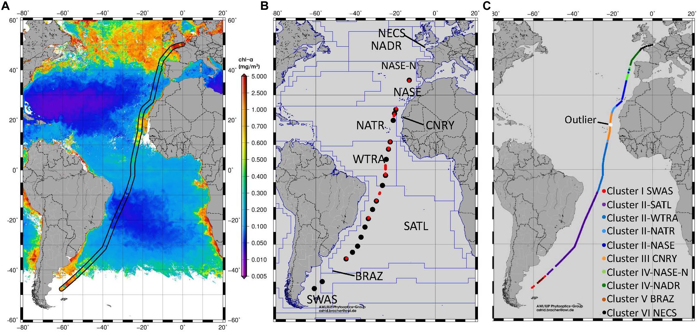
Figure 1. (A) Surface TChla determined from HPLC samples during PS113 and from satellite (Sentinel-3A OLCI GlobColour GSM-Chla level-3 daily 4 km products based on reduced resolution data version ESA PB2.3 products from the CMEMS GlobColour data archive, http://www.globcolour.info/). (B) Location of the radiometric profiles obtained at CTD stations (black dots) and at Triaxus casts (red dots) during PS113. The biogeochemical provinces according to Longhurst (2007) are marked and the provinces crossed by our cruise are named. SWAS for Southwest Atlantic Shelves, BRAZ for Brazilian Current Coast, SATL for South Atlantic Tropical Gyre, WTRA for Western Tropical Atlantic, NATR for North Atlantic Tropical Gyre, CNRY for Canary Current Coast, NASE North Atlantic Subtropical Gyre East, NASE-N for Northern NASE, NADR for North Atlantic Drift and NECS for Northeast Atlantic Shelves. (C) Distribution of HPLC surface stations into different clusters after applying hierarchical cluster analysis following Taylor et al. (2011). Clusters I, III, V, and VI are associated with Longhurst provinces, as defined in (B). Clusters II and IV were further differentiated after considering the significant differences for surface TChla, temperature and salinity within the two clusters which also reflect certain Longhurst Provinces. One outlier within CNRY province was identified which had been organized to cluster V (BRAZ).

The water samples were filtered on board through Whatman GF/F filters and the filters were thermally shocked in liquid nitrogen and stored in the −80°C freezer. The filters were brought to the Alfred-Wegener-Institute after arrival in Bremerhaven within a dry-ice filled box. The soluble organic phytoplankton pigment concentrations were determined using HPLC according to the method of Barlow et al. (1997) adjusted to our temperature-controlled instruments as detailed in Taylor et al. (2011). We determined the list of pigments shown in Table 2 of Taylor et al. (2011) and applied the method by Aiken et al. (2009) for quality control. Uncertainties of our HPLC measurements were assessed from triplicate samples taken at several prior cruises (data sets related to Taylor et al., 2011; Zindler et al., 2013; Bracher et al., 2015). For the different cruises the average deviation for HPLC analyses ranged from 5 to 8% with a standard deviation for triplicates between 1 and 11%.

The Chla of the main PGs [diatoms, dinoflagellates, haptophytes, prokaryotic phytoplankton excluding Prochlorococcus (for brevity now called cyanobacteria), chlorophytes, cryptophytes, and chrysophytes] were calculated based on diagnostic pigment analysis (DPA) developed by Vidussi et al. (2001) for PSCs Chla, further refined to calculate PGs Chla in Hirata et al. (2011). We followed Losa et al. (2017, Supplementary Material) for the pigment specific coefficients as applied in Booge et al. (2018): The fractions of seven main phytoplankton groups (as listed above) were calculated based on the weighted sum of specific diagnostic pigments. These weights were based on coefficients derived from a large in situ pigment database excluding the Southern Ocean to convert each diagnostic pigment concentration into a group specific Chla. The Chla of Prochlorococcus was directly given by the divinyl-Chla. The total Chla (TChla) was determined from the sum of monovinyl- and divinyl-Chla and chlorophyllide a concentration.

Hyperspectral AOP and Euphotic Depth Data

Three types of AOPs and the euphotic depth, Z_eu, were calculated from measurements of depth (z) resolved hyperspectral downwelling irradiance spectra, E_d(z, λ). Two identical irradiance radiometers (RAMSES ACC-2-VIS, TriOS GmbH, Germany) covering a wavelength range of 320–950 nm with an optical resolution of 3.3 nm and a spectral accuracy of 0.3 nm were installed on two different platforms:

The first radiometer was mounted to a steel frame system and then was lowered by a winch in about 5 m horizontal distance to the ship to measure the underwater E_d(z, λ) at 19 discrete stations at around 2 h before or after local noon and just before the CTD stations (Figure 1B). We followed the procedure described in Taylor et al. (2011). This radiometer was also equipped with an inclination and a pressure sensor. To avoid ship shadow, the ship was oriented such that the sun was illuminating the side where the measurements were taking place. Radiometric profiles were collected down to the maximum where light could be recorded, except for one station with light below 135 m, at which point we had to stop the measurement at this depth due to the length of our cables. During each cast, the instrument was adapted to sea temperature for about 3 min at the subsurface and then lowered with 0.1 m/s to the maximum depth with waiting for about 1 min at each 5 m step until 40 m and then with 10 m steps until the maximum depth.

The second radiometer was mounted to a large undulating platform (Triaxus, extended version, MacArtney, Denmark) towed behind the ship at an average velocity of about 8 knots (4.1 m/s) for several transects within the cruise track. In the beginning of every transect the platform was hold for several minutes in the subsurface, then the platform was undulating between surface (varying with a minimum depth between 1 and 20 m) and about 250–300 m. The depth was recorded continuously by the pressure sensor of a Seabird CTD (Sea-Bird Electronics, United States) attached to the Triaxus and the inclination in either dimension was measured by the Triaxus hardware. E_d(z, λ) was measured by the RAMSES sensor and the average speed to lower or lift the platform was about 1 m/s. For more details on the operation of the Triaxus we refer to Strass (2018) and von Appen et al. (2020). The sensor meta data is available at https://hdl.handle.net/10013/sensor.5c126f5b-86de-469c-adf7-251789e54362 and the repository of the raw data is von Appen et al. (2019). Only profile data reaching Z_eu and with values of E_d(z = 15 m, λ = 490) > 150 mW m^–2 nm^–1 were further used in the processing. In total, we used the RAMSES profile data from 11 Triaxus transects, each of them lasting between 2 and 48 h (Figure 1B).

E_d(z, λ) measurements were collected with sensor-specific automatically adjusted integration times (between 4 ms and 8 s). For the station sensor data we used only the downcast data (since up and downcast were at the same geolocation), while for the Triaxus sensor data we used all available and suitable up- and downcast data since they were never at the same geolocation. For valid E_d(z, λ) data, the inclination in either dimension was smaller than 14° (Matsuoka et al., 2007). Following the NASA protocols (Mueller et al., 2003), E_d(z, λ) data were corrected for incident sunlight variations using simultaneously obtained downwelling irradiance at the respective wavelength measured above the surface water [E_d(0⁺, λ)] with another hyperspectral RAMSES ACC-2-VIS sensor. Finally, these data were interpolated on discrete intervals of 1 m. As surface waves strongly affect measurements in the upper few meters, deeper measurements that are more reliable can be further extrapolated to the sea surface (Mueller et al., 2003). Following Stramski et al. (2008), each profile was checked and an appropriate depth interval z′ was defined (for station data mostly 7–22 m and for the Triaxus casts mostly 7–30 m, sometimes even 7–60 m). This was used to calculate the mean diffuse attenuation coefficients for downwelling irradiance over this depth interval [Ǩ_d(λ)]. By using Ǩ_d(λ), the subsurface irradiance E_d(0^–, λ) for each profile was extrapolated from the profiles of E_d(z, λ) within the respective depth interval. Then two other types of AOP were calculated:

• The hyperspectral transmission at each depth was calculated as in Eq. (1):

• The vertical attenuation coefficients for downwelling irradiance, [i.e., K_d(λ, z_{1 →} z₂)] from the surface to the maximum light depth were calculated following Lee et al. (2005) for a 5 m interval between depths z₁ and z₂.

In order to derive Z_eu, the photosynthetic active radiation E_dPAR(z) was calculated as the integral over E_d(λ, z) for λ = 400 to 700 nm, respectively. For the depths above the upper limit of the respective depth interval the E_dPAR(z) fitted results and for the depths below the originally measured E_dPAR(z) values were taken. Finally Z_eu at each station was calculated from the E_dPAR profiles as the 1% light depth where E_dPAR(z) equals 0.01 of E_dPAR(z = 0 m).

EOF Based Prediction of Phytoplankton Groups From Hyperspectral Underwater Data

We modified the method developed by Bracher et al. (2015) which is similar to Xi et al. (2020) to derive continuous profile data of PG Chla and TChla. However, instead of using remote sensing reflectance we tested our three hyperspectral AOP data sets, T(z,λ), K_d(z_{1 →} z₂,λ), and Ǩ_d(λ), as spectral input to the models. We briefly summarize here this procedure and just detail our applied changes to the method by Bracher et al. (2015).

Step 1: We limited the spectral range of our AOP input data to 400–580 nm since the values at wavelengths above were often very noisy. We applied an EOF analysis to our standardized (subtracting the mean and then divided by the standard deviation) spectral AOPs. Standardized AOP spectra were matched for each PG separately with the HPLC based PG Chla data. Then the singular value decomposition was performed to the spectral AOP matrix X (with M observations × N wavelengths; M may vary among different PGs due to the number of matchups) to obtain the EOF modes by extracting the vectors of the scores associated with the EOF modes (U), the EOF loadings (V, i.e., spectral patterns) and the singular values of X on the diagonal in decreasing order (Λ):

Step 2: For each PG, we subsequently developed the corresponding multiple linear regression model using the collocated PG Chla data and the EOF modes extracted from the AOP data, in which the log-transformed PG Chla data derived from the HPLC measured pigment concentrations, $\text{ln}({\text{C}}_{\text{o}}^{\text{train}})$, are expressed as a function of a subset of the EOF scores (U). As in Xi et al. (2020), the EOF modes with standard deviations (singular values from Λ) that are less than 0.0001 times the standard deviation of the first EOF mode were considered insignificant and thus omitted. Following Bracher et al. (2015) a stepwise routine was applied to search for smaller regression models (for each PG model) based on fewer prediction terms through minimization of the Akaike information criterion. The regression model for PG Chla [ln⁡(C_p)] predictions was expressed as:

Step 3: The robustness of the fitted model was estimated following Bracher et al. (2015) by a cross-validation of the model fitting using 500 permutations for splitting the collocated data into two subsets, in which 80% of the data was used for model fitting (training), while the rest of the data was used for prediction validation (details in Step 4). The pairs of observed and predicted PG Chla ($C_o^{\text{val}}\text{and}{C}_p^{\text{val}}$, respectively) of the 500 permutations were recorded for later prediction error statistics.

Step 4: To predict PG Chla from the T(z, λ), K_d(z_{1 →} z₂,λ), and Ǩ_d(λ) spectral data for which we do not have corresponding pigment based PG information, we projected these standardized spectral data onto the EOF loadings (V) to derive the new sets of EOF scores (U). The derived U were subsequently used for the prediction with the fitted linear model [Eq. (3) in Step 2], where the regression coefficients were taken from the model developed with the full matchup data set of pigment and AOP [either T(z, λ), K_d(z_{1 →} z₂, λ), or Ǩ_d(λ)] data.

Step 5: We finally applied a strict data quality control since we encountered large deviations between the TChla directly predicted from its specific EOF model and the sum of the seven PG Chla predictions (SPG-Chla) for some data points. Cryptophyte Chla was not included because of the failure of reliable predictions and their marginal contributions as derived from the HPLC PG data (details see section “Prediction of Phytoplankton Groups From Hyperspectral Underwater Measurements”). We removed all data points where the deviation between SPG-Chla to TChla was larger than 20%. For Ǩ_d(λ) related predictions 42 out of 425 data points had to be removed, for the T(z, λ) and K_d(z_{1 →} z₂, λ) related predictions only one entire profile and only very deep measurements of profiles had to be removed. For K_d(z_{1 →} z₂, λ) related predictions deepest quality controlled data were 20–30 m above the deepest quality controlled T(z, λ) related predictions. Visual inspection showed that flagged Ǩ_d(λ) data had resulted from profiles where only very few data points were available within the upper layer and therefore the fitting of K_d in the upper depth failed. The remaining data sets showed a correlation coefficient of 0.93, 0.92, and 0.95 for T(z, λ), K_d(z_{1 →} z₂, λ), and Ǩ_d(λ) related predictions of TChla versus SPG-Chla, respectively. Finally the PG Chla (PG_i-Chla) was recalculated to agree consistently with TChla predictions, as follows. First, the fraction of each PG (f-PG_i) was determined by Eq. (4):

Then the final PG_i-Chla was determined by Eq. (5):

Statistical Assessment of Model Performance

Since the Chla range varied greatly among the different PG, we calculated mainly relative error statistics. Considering the comparison between HPLC observations and AOP data based model predictions, error statistics were calculated for the full collocated data set incorporated into the training (full-fit results). Here, the determination coefficient, R², the root mean square difference (RMSD), the slope and the intercept of the linear regression were based on the log-scaled predicted as compared to the log-scaled observed PG Chla and TChla data, while the median percent difference (MPD), the median percent bias (MPB) were based on the non-log-transformed concentrations. For the cross validation, the R² based on $\text{ln}(C_p^{\text{val}})$ versus $\text{ln}(C_o^{\text{val}})$ was derived for each permutation, and the mean value of the cross-validated R² (R²cv) for all permutations is calculated. Similarly, and in accordance with the error statistics above, the average of RMSD and MPD for cross validation, named RMSDcv and MPDcv, were determined. For exact definitions and equations see Bracher et al. (2015).

Temperature, Salinity, and Upper Mixed Layer

For further interpretation of our surface phytoplankton data set and clustering into biogeochemical provinces (see section “Classification of the Biogeochemical Provinces”), we compared these to matchup data of surface temperature and salinity obtained continuously during PS113 by the ship’s thermosalinograph Seabird SBE 21 equipped with an external thermometer SBE 38 (both Sea-Bird Electronics, United States) installed at the keel of the ship. These data are published in Strass and Rohardt (2018). Temperature and salinity profiles were obtained using a Seabird SBE 911 CTD (Sea-Bird Electronics, United States) at the discrete CTD stations and another one on the Triaxus platform. The measurements from the two CTD systems agree very well (von Appen et al., 2020). The corresponding data are published in Strass (2019) and von Appen et al. (2019). Density was calculated from temperature and salinity profiles and the upper mixed layer depth (Z_m) was derived from those density profiles as the depth at which the density first exceeds the shallowest measured density by 0.125 kg/m³.

Classification of the Biogeochemical Provinces

Water samples were grouped in clusters according to the results of an unsupervised hierarchical cluster analysis (HCA) using the Euclidian distance as the distance measure and linking clusters following Taylor et al. (2011). The unsupervised HCA has been proven useful in Taylor et al. (2011) based on phytoplankton pigment composition for reflecting the measurements groupings into biogeochemical provinces according to Longhurst (Longhurst, 2007). As input data, we used the HPLC based fractions of PG Chla to TChla. As in Taylor et al. (2011), within clusters, differences in surface TChla, surface temperature and surface salinity were tested following an initial Shapiro–Wilk’s W test of normality. Normally distributed data were tested with the independent t-test and non-normally distributed data were tested with a Mann–Whitney-U-test. All tests were considered significant when p < 0.05.

Results and Discussion

Prediction of Phytoplankton Groups From Hyperspectral Underwater Measurements

We obtained 227 valid surface data points for PG Chla and TChla derived from HPLC measurements. Twenty-four of these data were sampled at the CTD stations where we also obtained information at five more depths. Details on the range and distribution of TChla and PG fraction are discussed in Section “Phytoplankton Composition Along the Atlantic Transect.” Spectral input data sets were based on 424 valid irradiance profiles for T(z, λ) and K_d(z_{1 →} z₂, λ) and 383 valid Ǩ_d(λ) data points. The composition and range of the three AOP type input data, namely the depth resolved T(z, λ) and K_d(z_{1 →} z₂, λ), and the upper surface layer mean Ǩ_d(λ) data, are shown as original and standardized spectra (Figure 2). Standardized spectra, that were used for the EOF analysis, look very much alike for the latter two AOP data sets, and show inverted spectral features between T(z, λ) and K_d(z_{1 →} z₂, λ) data. The EOF analyses identified the dominant modes of variance which can be interpreted as signatures in the optical properties of water constituents in the light lit water column. The first four modes of EOF already explain 99.29, 99.45, and 99.77% of the total variance for the T(z, λ), K_d(z_{1 →} z₂, λ), and Ǩ_d(λ) based PG prediction models (Table 1), with the first mode explaining 68.83, 71.77, and 84.39%, respectively. Other studies (e.g., Craig et al., 2012; Taylor et al., 2013; Bracher et al., 2015; Xi et al., 2020) have detailed the EOF modes selected for predictions of water constituents. They have investigated the underlying bio-optical signature that several EOF modes may carry. The distinct linkage between the EOF modes and the specific pigments or PGs was not identified, as the PG information cannot, to first-order, be reflected by these EOF modes (Craig et al., 2012). We followed Bracher et al. (2015) and Xi et al. (2020) where not only TChla but also pigment concentrations and PG Chla were predicted, respectively, by including in the prediction models higher EOF modes. Though these contributed only a minute portion to the total AOP variance, they still might inherit the optical signatures of phytoplankton (partly group specific) pigments. Applying the Akaike information criterion (i.e., the significance of an EOF mode in terms of each term’s removal for each specific PG or TChla model, see Table 2), proved that for our models also higher EOFs still were significant for the predictions. All our models follow the EOF mode selections found for case-1 waters in Bracher et al. (2015) and Xi et al. (2020) where most of the variation in the spectral shape was caused by phytoplankton pigments (groups) absorption in addition to water absorption itself: E.g., the EOF-2 mode is the most important term for TChla and nearly all PG Chla models, except for Prochlorococcus and cyanobacteria where the other EOF modes take over and more EOF modes are included in these PG Chla models. This is because for these two groups their Chla does not co-vary with TChla.

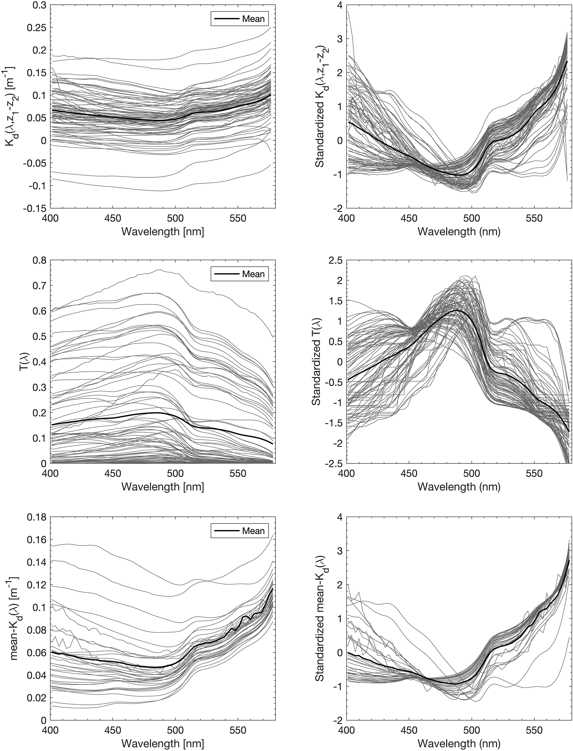
Figure 2. All spectra of the three types of AOP input data [upper panel: K_d(z_{1 →} z₂, λ), middle panel: T(z, λ), and lower panel: Ǩ_d(λ)] to EOF based PG and TChla prediction models. Spectra are provided as originals (left) and standardized by mean and standard deviation (right).

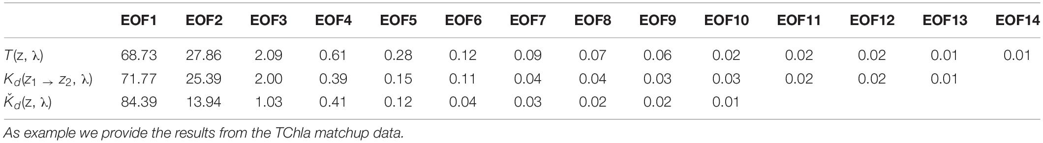
Table 1. Percentage of total variance explained by the decomposed EOF modes derived from the three PS113 AOP data sets T(z,λ), K_d(z_{1 →} z₂, λ) and Ǩ_d(λ), as specified in Sections “Hyperspectral AOP and Euphotic Depth Data” and “EOF Based Prediction of Phytoplankton Groups From Hyperspectral Underwater Data.”

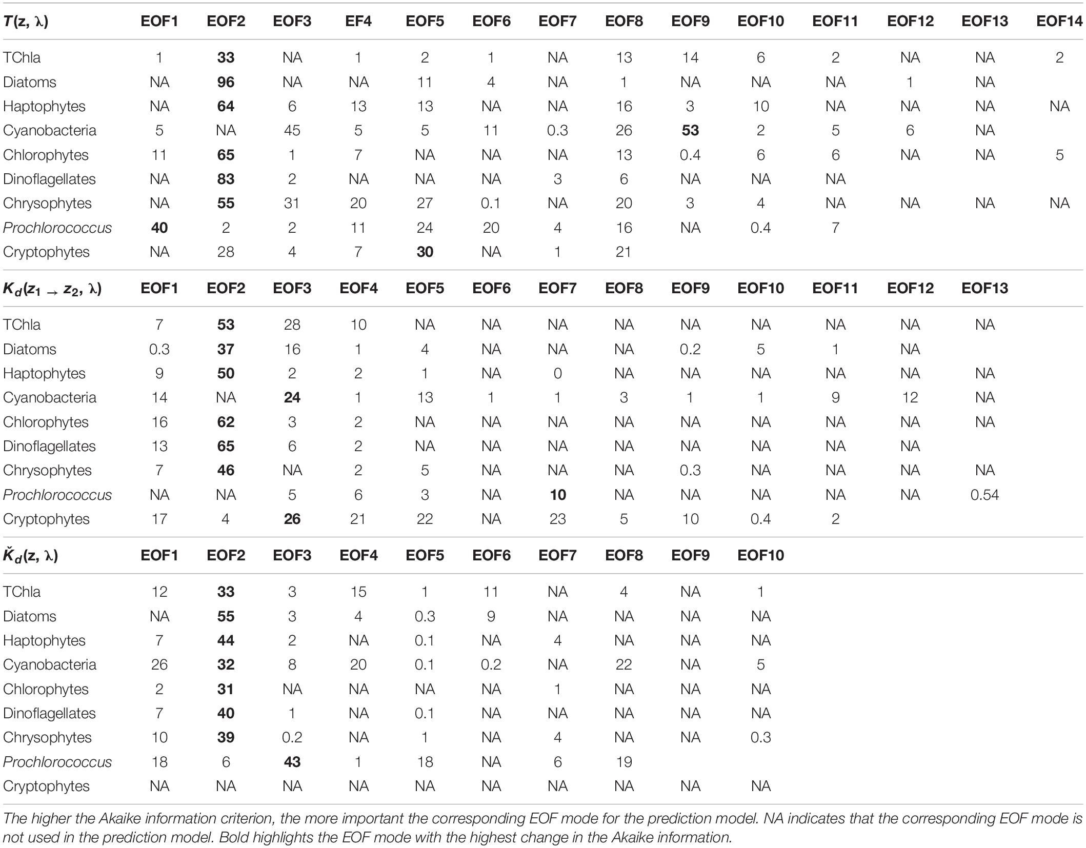
Table 2. Change in the Akaike information criterion for the robust PG Chla and TChla predictions by the EOF models based on three different types of AOP data sets [upper panel: T(z, λ), middle panel: K_d(z_{1 →} z₂, λ) and lower panel: K_d(λ)], as specified in Sections “Hyperspectral AOP and Euphotic Depth Data” and “EOF Based Prediction of Phytoplankton Groups From Hyperspectral Underwater Data.”

The results of the statistical assessment of the model performance considering the full fit and cross-validation comparisons are presented in Table 3. Matchups to HPLC PG data sets of the three AOP-derived PG Chla and TChla varied (Table 3), because for Ǩ_d(λ) only surface values, while for the T(z, λ) and K_d(z_{1 →} z₂, λ) data sets also matchups from CTD stations at five more depths could be considered. Different numbers of matchups for these two depth-resolved data sets resulted from the differences in valid PG data points due to the data quality procedure applied (see section “EOF Based Prediction of Phytoplankton Groups From Hyperspectral Underwater Data,” Step 5). Numbers of matchup data for distinct PGs were also different because certain PGs may not always be present at all matchup points. This is especially seen for cryptophytes which only gave ∼15% of matchups other groups gave. For the Ǩ_d(λ) data set, no predictions of cryptophytes were possible and for the T(z, λ) based data set the RMSDcv value became nearly five times higher than the RMSD value, both due to too limited number of cryptophyte matchups. Although the K_d(z_{1 →} z₂, λ) predictions of cryptophytes showed reasonable results for RMSDcv, R²cv, and MPDcv, we exclude this group from the further discussion and from predictions for the cruise transect, since the analysis by Bracher et al. (2015) clearly showed that a minimum of 25 matchup points are necessary for reliable pigment predictions.

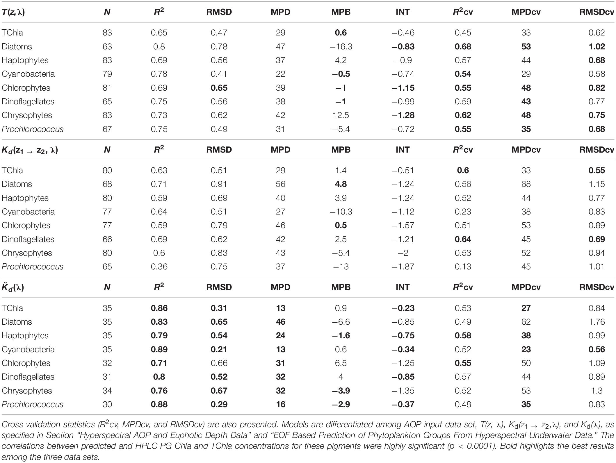
Table 3. Full fit statistics of PS113 optical based TChla and PG Chla predictions against HPLC TChla and PG Chla data: number of the matchup points (N), determination coefficient (R²), intercept (INT), median percent bias (MPB), median percent difference (MPD), and root mean square difference (RMSD).

All other PG Chla and TChla were well predicted from our regression models based on the EOF scores derived from the three hyperspectral AOP data sets combined with the matchup HPLC PG Chla (Table 3). Full fit results are best (indicated as bold in Table 3) for Ǩ_d(λ), closely followed by T(z, λ) and then K_d(z_{1 →} z₂, λ) based models (e.g., R² ≥ 0.71, ≥0.65 and ≥0.39, and MPD ≤ 46%, ≤47% and ≤56%, respectively). In addition, the results for the cross validation statistics based on 500 permutations using different sub-samples are similar for the three AOP data set based models. Full fit R², RMSD, and MPD values show better results for all three AOP based PG data sets as compared to R²cv, RMSDcv, and MPDcv values, respectively. However, for the T(z, λ) based PG data sets, the difference between the statistics of the full fit and that of the mean of the cross validation is lowest (here R²cv ≥0.54 and MPDcv ≤ 53%). Only its TChla prediction is a bit worse than for the two other AOP based models. For the K_d(z_{1 →} z₂, λ) based models, results for all three cross validation parameters are only slightly worse than T(z, λ) based models for most PGs, except for Prochlorococcus and cyanobacteria where they show very low prediction capabilities (e.g., R²cv of 0.13 and 0.23, respectively). For Ǩ_d(λ) based PG Chla data, the R²cv and MPDcv results are very similar to the T(z, λ) based model results, however, the RMSDcv values highlight large deviations for TChla and most PGs (except Prochlorococcus and cyanobacteria). As compared to RMSD, these values are increased mostly by a factor between 1.7 and 3, while the factor was only 1.2–1.4 and 1.1–1.7 for the T(z, λ) and K_d(z_{1 →} z₂, λ) based models, respectively. This indicates a lower stability for K_d(λ) based PG Chla and TChla data. It also emphasizes the need to consider a fleet of statistical parameters when assessing algorithm performance. Although the T(z, λ) data always bear spectral signatures caused by the scattering of light responding to the composition of water constituents from above layers to the respective depth (Lee et al., 2005), the retrieved PG Chla distributions from our model predictions based on this AOP data set also reveal realistic expectations of phytoplankton composition at deeper depths based on our cross validation results (The PG Chla and TChla predictions are further assessed and compared in sections “Phytoplankton Composition Along the Atlantic Transect”3.2 and “Comparison to Other Atlantic Ocean Observations of Phytoplankton Composition”). The shapes of standardized spectra of our T(z, λ) and K_d(z_{1 →} z₂, λ) data are just inverted and give the impression to contain very similar information (Figure 2). This leads to the conclusion that the introduced uncertainty from layers above to the defined layer depths of T(z, λ) is very low. The T(z, λ) data appear to be less affected by noise at low light levels since valid PG Chla predictions could be obtained at larger depths than the K_d(z_{1 →} z₂, λ) based model predictions. This is also supported by the recommendation of Lee et al. (2005) to rather choose a large depth interval for the calculation of K_d(z_{1 →} z₂, λ) in order to overcome the noise generated by wave introduced light fluctuations or high noise at low light levels. Therefore, given the fact that T(z, λ) data set provides overall the best cross validation statistics and that T(z, λ) based PG Chla and TChla data contain vertically resolved information reaching the deepest layers compared to those derived from the two other AOP variables, we selected this data set as being the most reliable data set. In the following we only use the predicted PG Chla and TChla data sets by T(z, λ) based models for comparison to similar data sets in other studies. Furtherone, we use this (now called ‘optical based prediction’) data set for demonstrating its applicability for obtaining highly resolved information on the phytoplankton abundance and composition in the water column of the Atlantic Ocean.

Our cross validation parameters obtained from the optical based PG and TChla predictions show comparable values (e.g., R²cv of 0.45–0.68, MPDcv of 29–53% and RMSDcv of 0.58–1.02) to other studies that retrieve TChla and phytoplankton pigment concentrations from optical data sets. E.g., Bracher et al. (2015), using in a similar region the same type of prediction models but based on field remote sensing reflectance data, obtained for R²cv, MPDcv and RMSDcv values ranging from 0.35 to 0.80, 28 to 43%, and 0.48 to 0.82. Chase et al. (2013) and Liu et al. (2019) derived phytoplankton pigments (different types of chlorophylls and the two major carotenoid groups) in the global and Arctic Ocean, respectively, by applying the Gaussian band method to hyperspectral IOP data from underway spectrophotometry; their validation results gave MPD values between 36–53% and 21–34%, respectively. Applying the matrix inversion technique in Liu et al. (2019) to the same Arctic data set allowed for the quantification of more specific carotenoid pigments, however, with larger MDP values (37–65%). Sauzede et al. (2015) predicted fractions of PSC on TChla from fluorometric data using a neutral network based technique combined with the abundance based approach by Uitz et al. (2006). Their validation results for the three PSC predictions against independent HPLC data gave R² values between 0.58–0.72 and MPD values of 35–46%. Compared to Xi et al. (2020) who employed the EOF based PG prediction models to satellite (multispectral) remote sensing reflectance data, our cross validation results based on T(z, λ) EOF models are for all PG groups and TChla better, except that their R²cv value are slightly better for TChla and haptophytes (0.75 and 0.61, respectively). In summary, our validation results indicate similar data quality as for the aforementioned methods predicting information on various phytoplankton pigment concentrations and fractions of PSC. We obtain even better quality for our models as compared to the PG Chla predictions by Xi et al. (2020), which is especially the case for cyanobacteria and Prochlorococcus Chla. This may be caused by the higher regional consistency of our data sets, the hyperspectral data set giving more opportunities to find the best linear models for the predictions and that the HPLC data have been measured by only one laboratory which further reduces measurement uncertainty.

Phytoplankton Composition Along the Atlantic Transect

During our cruise in May–June 2018 transecting the Atlantic Ocean from the Patagonian Shelf to the English Channel, the surface water TChla from our HPLC data set ranged between 0.03 and 5.42 mg/m³. The HPLC TChla corresponded well to the satellite Chla derived from the Sentinel-3A OLCI within the same time frame (Figure 1A). To further characterize the phytoplankton composition and distribution along the cruise track, we discuss the results from our HPLC and optical based predictions PG data sets based on their clustering into the Longhurst provinces (Longhurst, 2007). In our study lowest (HPLC) TChla were 0.037 at the surface and 0.015 mg/m³ at depth which is above the values encountered in the clearest ocean waters (South Pacific Gyre) by Morel et al. (2007). The corresponding PG Chla can be smaller and since the detection limit of our HPLC system is 1 μg/m³, we still kept all PG Chla above this value in the data set. However, following Xi et al. (2020) we consider PG Chla below 0.005 mg/m³ to bear much larger uncertainty.

The hierarchical cluster analysis based on the HPLC PG data resulted in six clusters. The assignment of the HPLC surface stations into the clusters is depicted in Figure 1C. The location of the samples belonging to four of the six clusters reflected very well the geographic locations of specific Longhurst provinces from the Atlantic Ocean: Clusters I corresponded to the Southwest Atlantic Shelves (SWAS), Cluster III to the Canary Current Coast (CNRY), Cluster V to the Brazilian Current Coast (BRAZ), and Cluster VI to the Northeast Atlantic Shelves (NECS). Cluster IV stations fall into the North Atlantic Drift (NADR) and the Northern part of the North Atlantic Subtropical Gyre East (NASE-N). The remaining cluster contained all Atlantic Longhurst gyre regions crossed by our cruise, namely the South Atlantic Tropical Gyre (SATL), North Atlantic Tropical Gyre (NATR), the southern part of North Atlantic Subtropical Gyre East (here abbreviated as NASE), and the Western Tropical Atlantic (WTRA). By further testing within clusters II and IV the significance of the absolute values of the surface TChla, temperature and salinity, a clear north-to-south structure could be distinguished and we finally could separate Cluster II into SATL, WTRA, NATR, and NASE, and Cluster IV into NASE-N and NADR stations. As an outlier, one station within CNRY appeared within Cluster V (BRAZ).

Following the province assignment based on the HPLC derived surface PG data, our optical based predictions of PG Chla and TChla were classified into the aforementioned Longhurst provinces. PG data from HPLC and the optical based predictions show consistent patterns. This is also found for PG distributions at depths where they were observed (below this is detailed for the provinces SATL, WTRA, NATR, and CNRY). However, for a few of them (n = 7, all sampled on May 31, 2018) the upper part of each profile was following NATR PG composition, while the lower part was following CNRY PG composition, or vice versa. This is consistent with the fact that in this region water from the open ocean North Atlantic intermixed on small horizontal and vertical scales with water from the Canary upwelling system (von Appen et al., 2020). Most optical stations (Table 4) were sampled in WTRA (>40%), closely followed by SATL (∼35%), and 10% were sampled each for the CNRY and NATR provinces. Only very few optical profiles were available from NASE (n = 8) and only one each for SWAS and BRAZ. This diminishes the generality of the observed features in the vertical structure in these latter provinces. We obtained only surface HPLC based PG data and no optical measurements North of 36°N (Table 4). Therefore, NASE-N, NADR, and NECS can only be described briefly, while for the SATL, WTRA, CNRY, and NATR we can provide in-depth analysis.

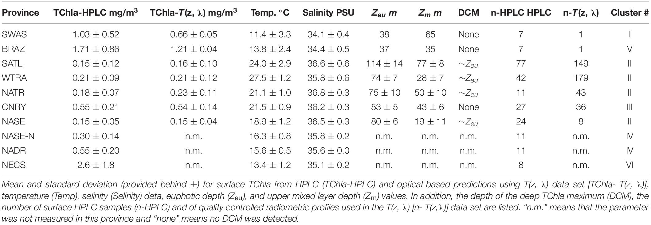
Table 4. Summary of PS113 measured parameters averaged within the Longhurst provinces, as clustered according to Figure 1B.

Mean and standard deviations (indicated as ±) for the fractions of PG Chla on TChla from the surface HPLC data are given in Table 5, and the surface HPLC-TChla, temperature and salinity measured from the thermosalinograph at all HPLC stations for each province are presented in Table 1. Figure 3 shows the depth resolved TChla along the whole cruise track from HPLC and optical based predictions. The latter match very well the values obtained from HPLC which is also supported by comparing the mean and standard deviation results in different Longhurst provinces for both data sets (Table 5). The optical based TChla predictions always reach at least the Z_eu (or even below), the depth where often the maximum biomass was obtained. Along our transect Z_eu ranged from ∼25–120 m and Z_m from 10 to 90 m. The surface PG Chla fraction predictions derived from the optical data set fall well within the standard deviation of fractions obtained from the HPLC data in all provinces (Figure 4). This is especially interesting as: (1) the optical data sampled two to three times more stations in the SATL, WTRA, CNRY, and NATR provinces (n = 149, n = 179, n = 43, and n = 36, respectively) than those by the HPLC data set (n = 77, n = 42, n = 13, and n = 13, respectively), and (2) the distribution of the sampled data was quite different for both data sets in these provinces. Mind that no robust predictions could be obtained for cryptophytes from the optical based data sets (see section “Prediction of Phytoplankton Groups From Hyperspectral Underwater Measurements”) while those were included in the calculation of the HPLC PG fractions. We do not expect this to introduce much uncertainty into the optical based PG fractions since the HPLC cryptophyte Chla data show that this group only contributed ∼10, ∼2, and ∼1% in SWAS, CNRY, and BRAZ, respectively, while they were absent in all the other provinces where we obtained optical data (Table 5).

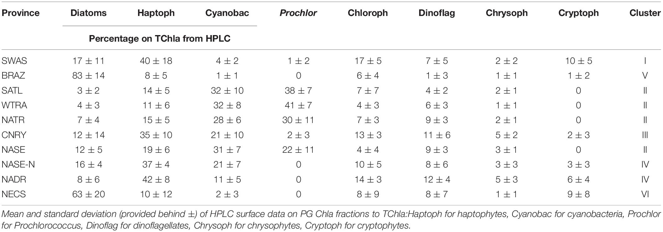
Table 5. Summary of PG Composition during PS113 within Longhurst provinces, as clustered according to Figure 1.

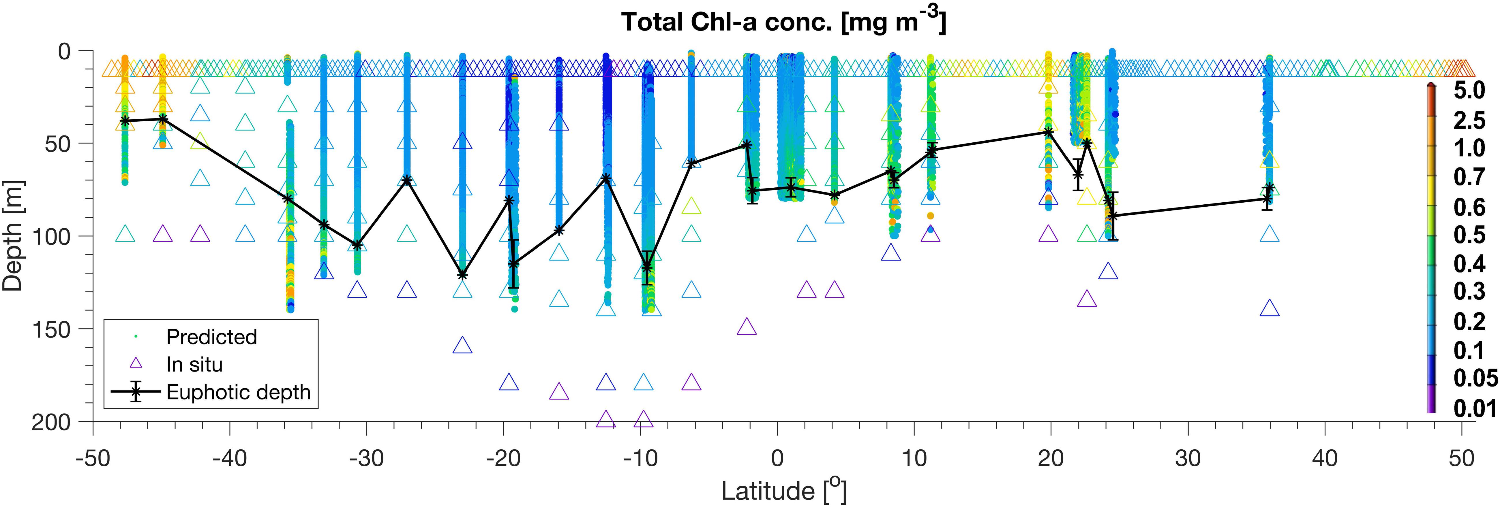
Figure 3. TChla from HPLC (triangle) and optical based [T(z, λ)] predictions (dots) within the water column along the whole PS113 transect. The euphotic depth, Z_eu, is also depicted (black line).

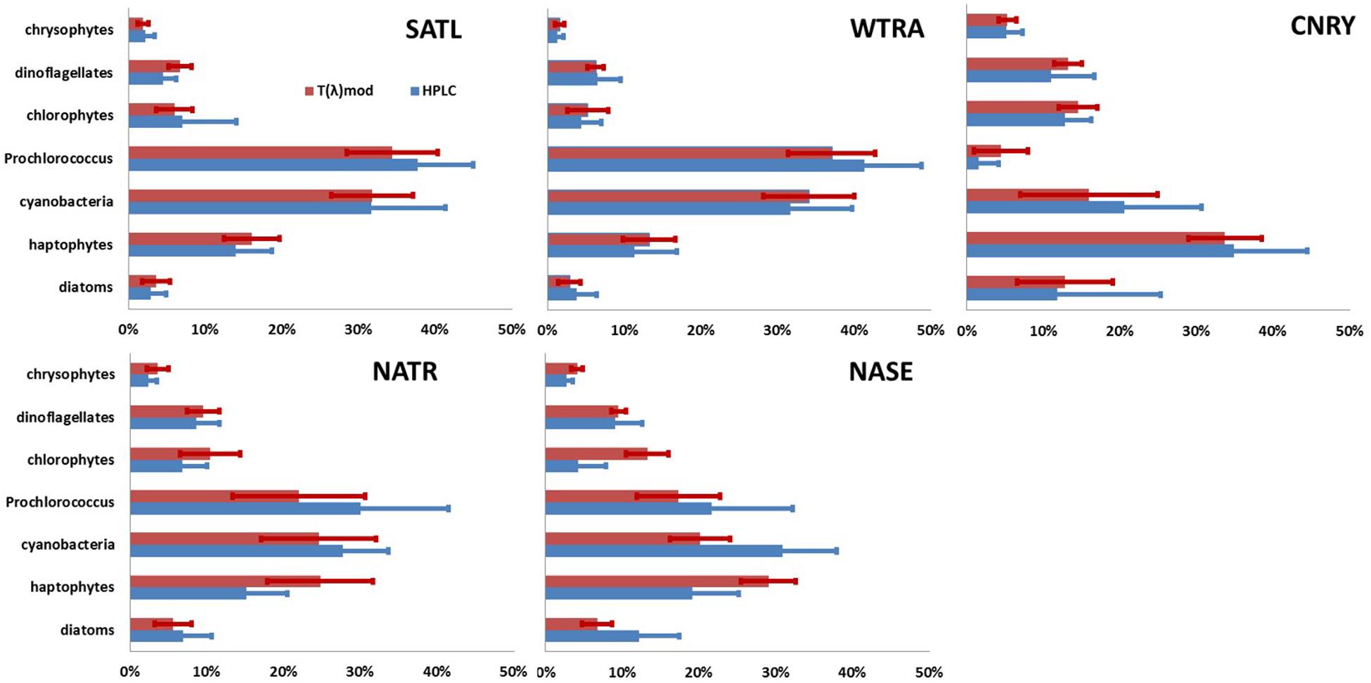
Figure 4. Mean (bar) and standard deviation (line) of fraction of seven PG Chla on TChla as obtained from HPLC data (blue) and optical based [T(z,λ)] predictions (red) during PS113 for the five Longhurst provinces SATL, WTRA, NATR, CNRY, and NASE, as defined in Figure 1. Cyanobacteria includes all prokaryotic phytoplankton without Prochlorococcus.

Moreover, at depth the optical based predictions of PG Chla agree well with the HPLC results within the four provinces (SATL, WTRA, CNRY, and NATR) where we collected four long continuous daylight optical profile samplings by our undulating platform Triaxus. They were carried out on 22, 24, 25, and 31 of May 2018 (Figures 5–7), respectively. Although we only obtained occasionally depth resolved HPLC PG Chla and TChla data (24 profiles in total with only six depths sampled each), we were able to derive 424 profiles of valid optical based prediction data at only a marginal ship time expense (the transit velocity of the ship had to be reduced from 10 knots to 8 knots). This high frequency vertical optical sampling provided the novel opportunity to resolve very well for these four Longhurst provinces the PG composition underneath the surface along the cruise track. Detailed discussion is presented below. If not referred to a specific figure, results can be found in Figure 4 and Tables 4, 5.

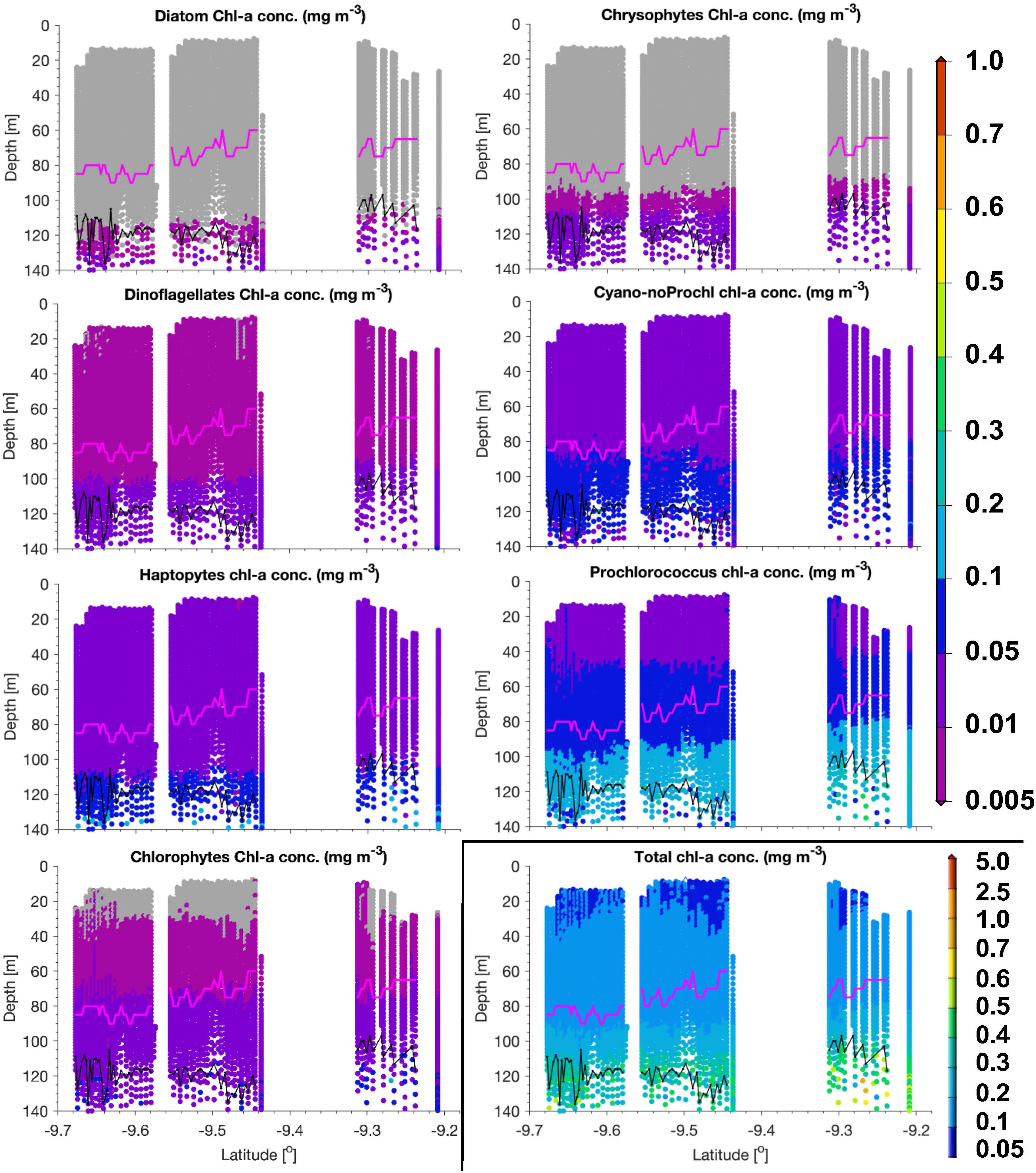
Figure 5. PG Chla and TChla from HPLC and optical based [T(z,λ)] predictions within the water column along a transect sampled with the Triaxus during PS113 on May 22, 2018 within the Longhurst province SATL. Mind that the color scale for TChla data is different from the one used for PG Chla. As in Figure 3, HPLC data are marked as triangles, optical based predictions as dots, euphotic depth Z_eu as black and the upper mixed layer depth Z_m as magenta line. Cyano-noProchl means cyanobacteria as defined in Figure 4. No TChla was detected below 0.05 mg/m³. Following Xi et al. (2020), PG Chla below 0.005 mg/m³ is flagged by gray color.

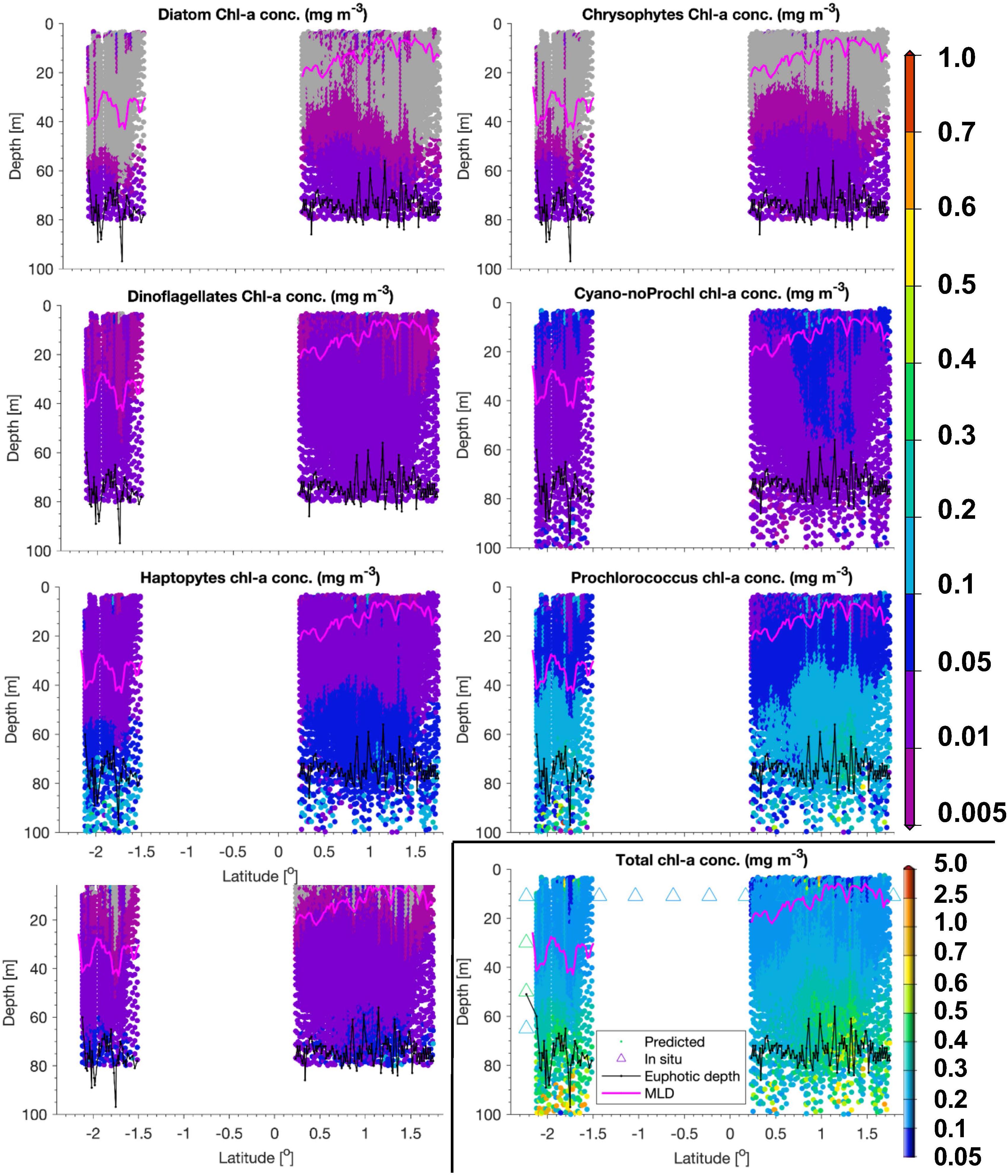
Figure 6. Same as Figure 5, but for a transect sampled on 24 and 25 May 2018 within the Longhurst province WTRA.

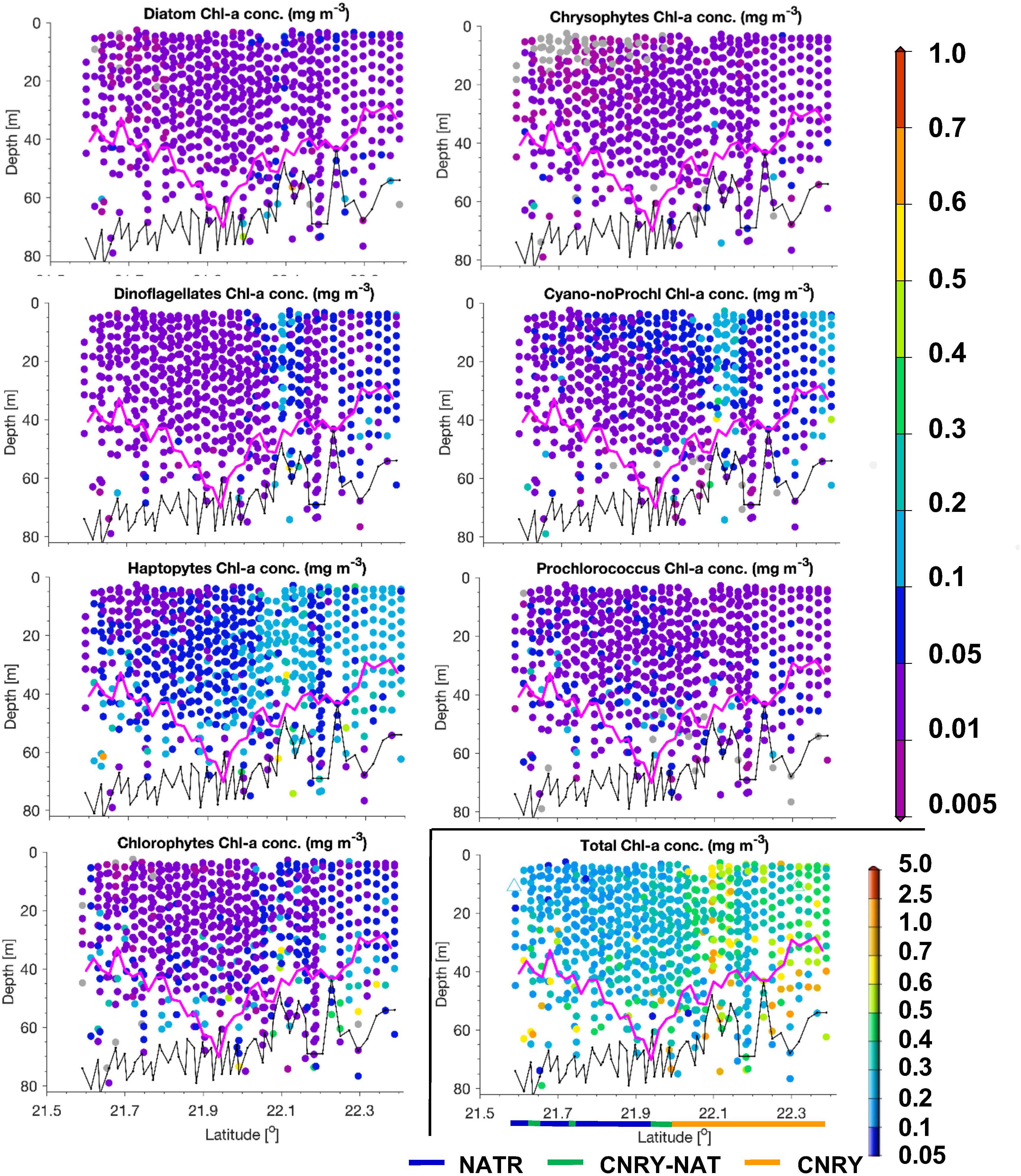
Figure 7. Same as Figure 5, but for a transect on May 31, 2018 within the Longhurst provinces NATR and CNRY. No TChla was detected below the threshold value of 0.05 mg/m³.

Within SATL, roughly from 42 to 27.5°S, surface TChla (0.15 ± 0.12 mg/m³ for HPLC based data, 0.16 ± 0.10 mg/m³ for optical based predictions) was the lowest (as in NATR), Z_eu and Z_m were the deepest (114 ± 14m and 77 ± 10 m, respectively) among all sampled Longhurst provinces. Salinity at surface was very high (∼36.6 PSU) as in the other gyre regions NATR and NASE, and surface temperature was around 24.0 ± 2.9°C. At surface, Prochlorococcus and cyanobacteria contributed about 40 and 35% to TChla, while haptophytes followed with ∼10%, and chlorophytes dinoflagellates and diatoms only contributed marginally. For the vertically highly resolved Triaxus cast in SATL (Figure 5), the biomass doubled in 20–40 m below the surface which was still about 20–40 m above the Z_m (∼60–80 m). It doubled again at about 10 m below the Z_m and reached the maximum within 20 m of the Z_eu (TChla maximum ∼0.2–0.35 mg/m³). Prochlorococcus Chla followed the overall biomass increase with depth and were always dominating. Cyanobacteria and chlorophytes only doubled below the Z_m. Haptophytes, chrysophytes, and dinoflagellates only doubled at the maximum chlorophyll layer around the Z_eu.

In WTRA, from about 8.5°S to about 10°N, surface TChla was slightly enhanced (0.21 ± 0.09 mg/m³ for HPLC based data, 0.21 ± 0.12 mg/m³ for optical based predictions) as compared to SATL, and the Z_eu and Z_m were about 40 and 50 m, respectively. As expected, surface salinity was lower than in the gyres (∼35.6 PSU) and surface temperature was the highest among all investigated provinces (27.5 ± 1.2°C). At the surface phytoplankton composition was about the same as in SATL. However, for the vertical profile the composition of phytoplankton changed (Figure 6). Here biomass doubled below the upper mixed layer and reached the TChla maximum (∼0.3 to <0.5 mg/m³) around 10–20 m within Z_eu. While cyanobacteria had maximum concentrations at the surface (mostly within the upper 10–20 m), Prochlorococcus followed TChla and dominated similarly TChla in the entire upper layer (∼40%). Below Z_m, haptophytes became the second dominant group. The other groups contributing only a minority at the surface, followed the TChla biomass distributions.

North of 10°N we crossed the more productive CNRY, which was twice intermitted by the NATR, which then finally at 24.5°N took over and ended around 25.5°N bordering to the NASE region. For a description of the dynamics of the intermixing of the different water masses in this section, see von Appen et al. (2020). Within NATR, surface TChla was nearly as low as in SATL (0.18 ± 0.07 mg/m³ for HPLC based data, 0.23 ± 0.11 mg/m³ for optical based predictions), Z_eu was about the same as for WTRA, but Z_m was significantly deeper (50 ± 10 m). While surface salinity was about the same as in SATL, the surface temperature was significantly lower than in WTRA (and SATL) with 21.1 ± 1.0°C. Prochlorococcus and cyanobacteria contributed less than in SATL and WTRA (about 25% each) and haptophytes nearly as much (∼20% of TChla), while diatoms, dinoflagellates and chlorophytes each reached ∼10%. The vertically highly resolved PG and TChla data (Figure 7) show that the TChla maximum was still found around the Z_eu, but only about double than the surface TChla. With depth the contribution of haptophytes increased and became the dominant group at the TChla maximum, while cyanobacteria clearly decreased with depth and Prochlorococcus showed more or less the same concentrations throughout the profile. The other PGs’ Chla (only minorly contributing) followed the distribution of haptophytes.

In CNRY, TChla was enhanced (0.55 ± 0.22 mg/m³ for HPLC, 0.54 ± 0.14 mg/m³ for optical predictions), but not reaching bloom conditions. Z_eu and Z_m were about 20 and 10 m, respectively, lower than in NATR. Surface temperature was about the same as in NATR, but surface salinity was a bit lower than in NATR and the other gyre regions (36.3 ± 0.3 PSU). At the surface haptophytes dominated by contributing about a third, followed by cyanobacteria contributing ∼20%, then followed by diatoms, chlorophytes and dinoflagellates with 10–15% and marginal contributions by chrysophytes, Prochlorococcus, and cryptophytes (≤5%). TChla was already high at the surface but often increased between Z_m and Z_eu. Contributions of the different PGs did not change at depth and followed the distributions of TChla (Figure 7).

In NASE, roughly from 25 to 36°N along the cruise transect, surface salinity was about as high (∼36.5 PSU) and TChla was as low (0.15 ± 0.05 mg/m³ for HPLC based data, 0.15 ± 0.04 mg/m³ for optical based predictions) as those observed in SATL. However, temperature was much lower (18.9° ± 1.2°C), and Z_eu was about 25 m shallower (∼80 m, but deeper than in NATR) than in SATL. Z_m were the shallowest (∼20 m) among the vertical profiles studied along our profiling transects. However, we have to keep in mind that the depth resolved sampling was limited in this province (only within 35.67–35.92 °N). The composition of the phytoplankton at surface was nearly the same as for the NATR, but the depth of the TChla maximum (here TChla was about twice the surface TChla) located at about 0–20 m above the Z_eu. Below the TChla maximum depth TChla decreased to surface levels and again increased at around 100 m to values equivalent to the TChla maximum (Figure 3). The composition of the phytoplankton at different depths (data not shown) corresponded to its composition at surface, except that cyanobacteria decreased below the upper mixed layer to <10%, and haptophytes and Prochlorococcus took up these contributions and dominated below.

Based on our surface HPLC station measurements only, the SWAS, BRAZ, NASE-N, NADR, and NECS were characterized as follows: Surface temperature and salinity in NASE-N and NADR (reaching from about 36 to 41°N and 42 to 48°N, respectively) further decreased compared to the tropical and subtropical regions (∼16.8 and 15.6°C, respectively, and ∼35.7 PSU). In NASE-N TChla was much enhanced with 0.30 ± 0.14 mg/m³ compared to NASE, but only about 50% of that in NADR (0.58 ± 0.2 mg/m³). Opposed to NASE, in both regions haptophytes dominated by ∼40% TChla and Prochlorococcus was absent. In NASE-N cyanobacteria contributed with ∼20% as the second dominant group before diatoms, in NADR chlorophytes and dinoflagellates contributed similarly as cyanobacteria, then followed by diatoms. Highest TChla along the Atlantic transect was found in the most southerly and the most northerly provinces, SWAS, BRAZ, and NECS, which are probably influenced by nutrient supply mainly from the continents (Marañón et al., 2001; Longhurst, 2007). In these regions surface temperature and salinity were the lowest among all provinces. TChla at the surface reflected bloom conditions (TChla > 1 mg/m³), but also the highest variation for surface TChla was obtained. Composition of phytoplankton was significantly different to the other regions. Diatoms were clearly dominating TChla at NECS and BRAZ stations. However, for SWAS stations, TChla was lower (∼1.0 mg/m³) and haptophytes became the dominating group (∼40%), while they were the second largest group with only around 10% contribution at NECS and BRAZ stations. The third largest group in SWAS and BRAZ were chlorophytes, while in NECS they shared this position with dinoflagellates and cryptophytes. For SWAS and BRAZ we can add our findings from one vertically highly resolved optical profile each (Figure 3). Here Z_eu at both stations was rather shallow (<40 m). Z_m was very shallow for the high biomass BRAZ station (35 m) and much deeper for the moderate biomass SWAS station (65 m). The maximum of TChla was at the surface reaching down to the Z_eu for both stations.

Comparison to Other Atlantic Ocean Observations of Phytoplankton Composition

The composition of phytoplankton obtained from our HPLC data and optical based predictions along the sampled Atlantic transect can be compared to previous point based PG surface Chla observations from HPLC verified with microscopic and flow cytometry data from Veldhuis and Kraay (2004), Taylor et al. (2011), and Nunes et al. (2019), and to pigment observations from Barlow et al. (2002). The Longhurst provinces sampled by the studies corresponded well to parts of our transect: Taylor et al. (2011) to the Northern part with NECS, NADR, NASE-N, NASE, and CNRY, Veldhuis and Kraay (2004) to NASE and NATR, Nunes et al. (2019) to the Southern part with NASE, CNRY, NATR, WTRA, SATL, and SWAS, and Barlow et al. (2002) to all provinces.

For the gyre regions SATL, NATR, NASE, and WTRA TChla, PG Chla and PG Chla contributions to TChla from our data agree well to the other studies, except that in WTRA, SATL, and NASE the contribution by cyanobacteria in our study is higher (∼30%) than in Taylor et al. (2011) and Nunes et al. (2019), ∼15 and ∼10%, respectively). Within NASE in Taylor et al. (2011) and Nunes et al. (2019) Prochlorococcus contribute more (∼40%), while in our study the contribution of Prochlorococcus is significantly less (∼25%). It may be due to that relating the zeaxanthin concentration just to monovinyl-Chla and chlorophyllide a concentrations to obtain cyanobacteria Chla in our method is not sufficiently accounting for the contribution of Prochlorococcus to zeaxanthin. This has been done in the two other studies by applying the CHEMTAX method (Mackey et al., 1996) adjusted for the tropical and subtropical Atlantic. However, when looking at Veldhuis and Kraay (2004) patterns for PG Chla (which were also retrieved from HPLC pigments using the adjusted CHEMTAX method), their data agree well both at surface and depth to our contributions of PG to TChla: Cyanobacteria have slightly higher contributions (≥30%) at the surface than Prochlorococcus and haptophytes (both ∼25%), while at the deep chlorophyll maximum cyanobacteria decrease to ≤10% and the other two groups dominate. At NATR, our results also agree with their contributions of PG Chla to TChla within the depth profile. In SATL and WTRA the contribution of haptophytes is higher in Nunes et al. (2019) (∼22% versus ∼15% from our study) and compensating the lower contribution of cyanobacteria; however, depth resolved results from Barlow et al. (2002) on zeaxanthin and divinyl-Chla (which are marker pigments for both, cyanobacteria and Prochlorococcus, and Prochlorococcus alone, respectively) indicate, that at the surface the contribution of cyanobacteria can be expected to be similar in SATL and WTRA and larger than in NASE. Their data set also supports the dominance of Prochlorococcus and haptophytes observed in all four provinces at the deep chlorophyll maximum as we have observed in our data set.

Results for the CNRY region differ the most among the studies: While Nunes et al. (2019) observe oligotrophic conditions with very low surface TChla (only ∼25% of our values), values in Barlow et al. (2002) and Taylor et al. (2011) are much higher (3.2 ± 1.7 mg/m³ and 1.5–2 mg/m³, respectively). In Nunes et al. (2019) the phytoplankton composition in CNRY is similar to NASE, except that Prochlorococcus decrease to ∼18% and diatoms increase to ∼15%. For Taylor et al. (2011), the composition is similar to what we obtained for NECS, with diatoms dominating by ∼60% the biomass, followed by haptophytes and cyanobacteria (here grouped as Synechococcus) with about 10–15%. In Barlow et al. (2002), diatoms and haptophytes are probably similarly contributing and cyanobacteria are contributing the least. Our surface TChla and PG composition seem to fall between the two extreme cases (Nunes et al., 2019, versus Taylor et al., 2011). Since CNRY is described as the province being affected by sporadic offshore filaments of nutrient-rich waters originating in the seasonal Northwest African coastal upwelling (Longhurst, 2007), the TChla can fluctuate a lot and phytoplankton composition can also change. Within our high resolution casts in this region and the associated NATR province (Figure 7), we also sampled other oceanographic physical and chemical parameters which are analyzed in von Appen et al. (2020), which clearly shows that our day time optical profiles are partly sampled in the CNRY province. While nutrients are depleted for most of the transect covered by the day time optical profiles, there are also a few locations where nutrients, though far below supporting phytoplankton bloom levels, could have supported the growth of phytoplankton. PG Chla and TChla in Nunes et al. (2019) also correspond well to our results from Cluster V (BRAZ) stations with similar TChla range and diatoms, followed by haptophytes and chlorophytes as main contributors at surface waters. Taylor et al. (2011) data from NECS, NADR, and NASE-N confirmed our surface TChla and PG Chla results based on HPLC data only. Some of the differences between our results and the other studies can probably be explained by the variations in different sampling seasons, years and specific areas within each province. Veldhuis and Kraay (2004) sampled in boreal summer, the other three studies sampled in boreal fall and austral spring, while we sampled austral fall and boreal spring. As expected, in Taylor et al. (2011) and Nunes et al. (2019) surface temperatures in NATR, CNRY, and NASE are much warmer – with mean values ∼3–6 and ∼2–3°C higher, respectively, while in the other provinces they are similar to ours. Salinity is much lower for NATR (35.8 ± 0.2 PSU) in Nunes et al. (2019), but similar for all other provinces and for all provinces sampled by Taylor et al. (2011). Within NASE, Taylor et al. (2011) have measured similar Z_eu but much deeper Z_m (∼80 m) than our study. Opposed to that, Veldhuis and Kraay (2004) data on TChla at maximum depth and Z_m are similar, but Z_eu is much deeper (NATR: 100–140 m, NASE: ∼130 m) compared to our data. Based on these comparisons of our phytoplankton high resolution data to the point data results obtained in the other studies, we conclude that our HPLC and especially our horizontally and vertically highly resolved optical based predictions show realistic distributions of phytoplankton abundance and composition in the sampled biogeochemical provinces.

Sources of Uncertainties in Our Optical Retrievals of Phytoplankton Composition

Several sources of uncertainties are related to our optical data based retrievals. We have quantified the retrieval errors by our cross validation results (see section “Prediction of Phytoplankton Groups From Hyperspectral Underwater Measurements”). With our quality control applied to the final optical based PG data (see section “EOF Based Prediction of Phytoplankton Groups From Hyperspectral Underwater Data” Step 5), we have reduced uncertainties introduced by inappropriate light radiation measurements. However, as recommended in Bracher et al. (2017) and IOCCG (2019) for retrieving PGs from optical measurements and empirical algorithms, respectively, we are missing the quantification of uncertainties introduced by the HPLC pigment measurement itself (including all associated steps, e.g., filtration, extraction and HPLC analysis accuracy), and by the representation error assigned to the DPA for grouping phytoplankton and quantifying PGs.

In the current study we could not include the source of error resulting from the input HPLC data set since we only were able to quantify uncertainty, based on our triplicate HPLC measurements (see details in section “Phytoplankton Group Biomass From Phytoplankton Marker Pigment Measurements”), arising from water sampling, filtration and extraction. We are currently assessing the uncertainty related to our HPLC analysis system within an international laboratory intercomparison activity on HPLC phytoplankton pigments (this round-robin is called HIP-5) which follows similar previous intercomparisons (Canutti et al., 2016).

Using HPLC phytoplankton pigments together with DPA for grouping of phytoplankton has the advantage that it covers the whole phytoplankton assemblage in a single analysis and provides a quantitative assessment of phytoplankton community composition at group level (Bax et al., 2001). In addition, the pigments directly determine phytoplankton absorption (e.g., Bidigare et al., 1989). However, defining PG Chla based on DPA (which is similarly true when using CHEMTAX to determine PG Chla, as used in some studies mentioned in section “Comparison to Other Atlantic Ocean Observations of Phytoplankton Composition”) bears the limitation that phytoplankton pigment composition is only to a certain degree congruent with taxonomy (Bracher et al., 2017). There is substantial variability in pigment concentration as a function of physiological response to environmental conditions. Besides, certain diagnostic pigments are present in several PGs (e.g., fucoxanthin in diatoms and haptophytes). The uncertainty introduced by using fucoxanthin as diagnostic pigment for diatoms was reduced for our data set by following the Hirata et al. (2011) fucoxanthin correction within our DPA. Still an error of not correctly quantifying PGs remains for our HPLC PG Chla data set, which we could not quantify, since we had no opportunity to sample for other, more precise, descriptors of phytoplankton taxonomic composition. All studies on the distribution of PGs and its composition in the Longhurst provinces (see section “Comparison to Other Atlantic Ocean Observations of Phytoplankton Composition”) that we compared our results to were validated with such data. Regarding the consistency of our results with these studies, we consider the uncertainty from both sources (HPLC measurement error and diagnostic pigment analysis representation error) to be low.

Conclusion and Perspective

We present robust predictions with high horizontal (∼1 km) and vertical (∼10 m) resolution to the Z_eu and deeper of seven PG (diatoms, dinoflagellates, haptophytes, cyanobacteria, Prochlorococcus, chlorophytes, and chrysophytes) Chla and TChla for several transects of 50–150 km length in the tropical and subtropical Atlantic Ocean. Additionally, for optical profiles measured at discrete stations, we obtained the same information on phytoplankton abundance and composition with very high vertical resolution (<1 m). These data are derived from first fitting EOFs to hyperspectral AOP data obtained from measurements in the water profile of spectral irradiance, either obtained as single profiles at discrete stations or continuously by a sensor mounted to an undulating platform towed behind the ship. Subsequently, multiple linear regression models were developed with HPLC pigment based phytoplankton group Chla as the response variable and scores from the selected EOF modes as predictor variables. These linear models were then applied to all hyperspectral AOP data measured continuously at the different transects in the Atlantic Ocean enabling us to observe (to our knowledge) for the first time, high horizontally and vertically resolved PG information from observations within four major biogeochemical provinces of the Atlantic Ocean. We obtain robust predictions for seven PG, that explain more than 95% of the total phytoplankton biomass in these provinces, which is shown by the results of cross-validation (R²cv of 0.54–0.68 and MPDcv of 29–53%) using statistical resampling (500 permutations). Our high horizontally and vertically resolved PG contributions to TChla within the Atlantic biogeochemical provinces as classified by Longhurst (2007) correspond well to previous results on phytoplankton composition from discrete water sample analysis via microscopy, flow cytometry, and HPLC marker pigments.

Although our data set bears several limitations (e.g., the non-proper propagation of measurement errors through the retrieval and the representation error, details in section “Sources of Uncertainties in Our Optical Retrievals of Phytoplankton Composition”), this high resolution information on phytoplankton diversity is one step toward closing the gap of knowledge in the distribution of phytoplankton groups, especially below the surface where sampling of phytoplankton diversity measures have been very scarce.

Our study shows the potential of employing radiometers on undulating platforms towed behind the ships at 8 knots which is only slightly below typical cruising speed. These undulating platforms can include a large range of big and power-hungry oceanographic sensors. E.g., in our case, information at the same horizontal and vertical resolution was also collected of temperature, salinity, velocity, oxygen, nitrate, and attenuation (more details in von Appen et al., 2020). Thereby, we can obtain novel and needed descriptors of upper ocean processes which goes beyond bulk parameters (Chlorophyll a and colored dissolved organic matter fluorescence, particle back scattering, photosynthetic active radiation or irradiance) as resolved by traditional IOP and AOP sensors. These sensors are already operated also on autonomous systems such as gliders or profiling floats.

The necessity for retrieving phytoplankton groups with high spectrally resolved data leads to a demand of high energy supply and high data recording rates. This can currently only be met by operation on a ship-towed undulating platform. The Triaxus system used in our study provides the possibility to operate many sensors at the same time (von Appen et al., 2020). Since the platform is rather big, also larger instrumentation [e.g., in addition to the radiometer, an AC-S (Sea-Bird Electronics, United States) during our campaign] and systems which require high energy supply and high data rate transfer (as it is the case for hyperspectral radiometers) can be installed. It enables the operation of both, IOP and AOP, hyperspectral instruments at the same time in addition to all the other traditional sensors. Although the vertical speed of the system was around 1 m/s (in addition to the 4 m/s horizontal speed) reliable spectral transmission data mostly until below the Z_eu could be obtained. The depth limit until where information can be obtained is clearly dependent on incident light which was very high during our undulating platform operations in the tropics and subtropics. In the future obtaining PG Chla and TChla data from hyperspectral IOP sensors would be favorable and should be explored because radiometers only provide valid data under daylight (leading to the absence of AOP information in our transects during night-time), while IOP instruments use their own light source. However, hyperspectral IOP sensors need even higher energy supply than the radiometers. The later have the advantage to be rather self-calibrating since AOPs are derived. Cross-calibration of IOP and AOP sensor data and of their associated data sets on phytoplankton composition can facilitate reliable calibration of hyperspectral IOP sensors which up to now is a big challenge (see IOCCG Protocol Series, 2019).

The prospect would be to put in future similar radiometers on profiling floats or gliders which would enable the large scale collection of vertically resolved phytoplankton data at much improved horizontal coverage. But before this can be implemented, the challenges on energy supply and big data recording must be met in addition to reducing the size of radiometers in order to fit them onto these platforms. For now it seems warranted to obtain towed hyperspectral AOP measurements along transects that are anyways occupied by research vessels.

Data Availability Statement

The HPLC pigment and PG data and the AOP based PG Chla model predictions are stored at https://doi.pangaea.de/10.1594/PANGAEA.913536, references are detailed as Bracher et al. (2020a,b,c,d). All other data are already publicly available as cited in Section “Materials and Methods.”

Author Contributions

AB designed the study, developed the method, analyzed RAMSES and HPLC data, and wrote the manuscript. AB, HX, and SW collected the water samples for HPLC and measured RAMSES data. SW measured HPLC samples. HX quality controlled HPLC data, contributed to EOF analysis, and made most figures of the manuscript. AM provided OLCI level-3 GlobColour products. W-JA and VS designed the operation and ran the ship-towed undulator. W-JA and VS provided the UML data from the CTD data. TD wrote part of the RAMSES data processing software. All co-authors substantially commented on the manuscript.

Funding

Support for this study was provided by the Helmholtz Infrastructure Initiative FRAM. Ship time was provided under grant AWI_PS113_00. HX’s participation in PS113 was supported via the project ACRI/OLCI-PFT.

Conflict of Interest

The authors declare that the research was conducted in the absence of any commercial or financial relationships that could be construed as a potential conflict of interest.

Acknowledgments

We thank H. Becker, S. Spahic, J. Hagemann, and S. El Naggar for their invaluable help in collecting the Triaxus data presented here. The CTD at the hydrographic stations was operated by H. Leach and J. Gerken. We thank B. Bracher for supporting HPLC sample analysis and the captain, the crew and other scientists on board PS113 for their valuable support on board. We thank ESA, EUMETSAT, and CMEMS GlobColour program for providing OLCI Chla level-3 products.

References

Aiken, J., Pradhan, Y., Barlow, R., Lavender, S., Poulton, A., Holligan, P., et al. (2009). Phytoplankton pigments and functional types in the Atlantic Ocean: a decadal assessment, 1995–2005. Deep-Sea Res. II Top. Stud. Oceanogr. 56, 899–917 doi: 10.1016/j.dsr2.2008.09.017
Barlow, R. G., Aiken, J., Holligan, P. M., Cummings, D. G., Maritorena, S., and Hooker, S. (2002). Phytoplankton pigment and absorption characteristics along meridional transects in the Atlantic Ocean. Deep Sea Res. I Oceanogr. Res. Pap. 49, 637–660. doi: 10.1016/S0967-0637(01)00081-4
Barlow, R. G., Cummings, D. G., and Gibb, S. W. (1997). Improved resolution of mono-and divinyl chlorophylls a and b and zeaxanthin and lutein in phytoplankton extracts using reverse phase C-8 HPLC. Mar. Ecol. Prog. Ser. 161, 303–307. doi: 10.3354/meps161303
Bax, N. J., Burford, M., Clementson, L., and Davenport, S. (2001). Phytoplankton blooms and production sources on the south-east australian continental shelf. Mar. Freshw. Res. 52, 451–462. doi: 10.1071/MF00001
Bidigare, R. R., Morrow, J. H., and Kiefer, D. A. (1989). Derivative analysis of spectral absorption by photosynthetic pigments in the western Sargasso Sea. J. Mar. Res. 47, 323–341. doi: 10.1357/002224089785076325
Booge, D., Schlundt, C., Bracher, A., Endres, S., Zäncker, B., and Marandino, C. A. (2018). Marine isoprene production and consumption in the mixed layer of the surface ocean – A field study over 2 oceanic regions. Biogeosciences 15, 649–667. doi: 10.5194/bg-15-649-2018
Bracher, A., Bouman, H. A., Brewin, R. J. W., Bricaud, A., Brotas, V., Ciotti, A. M., et al. (2017). Obtaining phytoplankton diversity from ocean color: a scientific roadmap for future development. Front. Mar. Sci. 4:55. doi: 10.3389/fmars.2017.00055
Bracher, A., Taylor, M. H., Taylor, B., Dinter, T., Röttgers, R., and Steinmetz, F. (2015). Using empirical orthogonal functions derived from remote-sensing reflectance for the prediction of phytoplankton pigment concentrations. Ocean Sci. 11, 139–158. doi: 10.5194/os-11-139-2015
Bracher, A., Vountas, M., Dinter, T., Burrows, J. P., Röttgers, R., and Peeken, I. (2009). Quantitative observation of cyanobacteria and diatoms from space using PhytoDOAS on SCIAMACHY data. Biogeosciences 6, 751–764. doi: 10.5194/bg-6-751-2009
Bracher, A., Wiegmann, S., and Xi, H. (2020a). Phytoplankton Pigment Concentration and Phytoplankton Groups Measured on Water Samples Obtained during POLARSTERN Cruise PS113 in the Atlantic Ocean. PANGAEA. doi: 10.1594/PANGAEA.911061
Bracher, A., Xi, H., and Dinter, T. (2020b). High resolution phytoplankton group Chlorophyll a data derived using transmission from high spectrally resolved radiometric underwater light profiles at discrete light stations obtained during POLARSTERN cruise PS113 in the Atlantic Ocean. PANGAEA. doi: 10.1594/PANGAEA.913514
Bracher, A., Xi, H., and Dinter, T. (2020c). High resolution phytoplankton group Chlorophyll a data from high spectrally resolved radiometric underwater light transmission profiles obtained by an undulating platform towed behind the ship during POLARSTERN cruise PS113 in the Atlantic Ocean. PANGAEA. doi: 10.1594/PANGAEA.913517
Bracher, A., Xi, H., and Dinter, T. (2020d). Phytoplankton group Chlorophyll a data derived using the mean diffuse attenuation over the first optical depth (kdmean) of the measured radiometric profile obtained during POLARSTERN cruise PS113 in the Atlantic Ocean. PANGAEA. doi: 10.1594/PANGAEA.913520
Bricaud, A., Ciotti, A. M., and Gentili, B. (2012). Spatial-temporal variations in phytoplankton size and colored detrital matter absorption at global and regional scales, as derived from twelve years of SeaWiFS data (1998–2009). Glob. Biogeochem. Cycles 26:GB1010. doi: 10.1029/2010GB003952
Brotas, V., Brewin, R. J. W., Sá, C., Brito, A. C., Silva, A., Mendes, C. R., et al. (2013). Deriving phytoplankton size classes from satellite data: validation along a trophic gradient in the eastern Atlantic Ocean. Remote Sens. Environ. 134, 66–77. doi: 10.1016/j.rse.2013.02.013
Canutti, E., Ras, J., Grung, M., Roettgers, R., Costa Goela, P., Artuso, F., et al. (2016). HPLC/DAD Intercomparison on Phytoplankton Pigments (HIP-1, HIP-2, HIP-3 and HIP-4). Available online at: https://www.researchgate.net/publication/321491410_HPLCDAD_Intercomparison_on_Phytoplankton_Pigments_HIP-1_HIP-2_HIP-3_and_HIP-4/link/5a256a7e4585155dd41f821a/download (accessed April 1, 2020).
Chase, A., Boss, E., Zaneveld, R., Bricaud, A., Claustre, H., Ras, J., et al. (2013). Decomposition of in situ particulate absorption spectra. Methods Oceanogr. 7, 110–124. doi: 10.1016/j.mio.2014.02.002
Craig, S. E., Jones, C. T., Li, W. K. W., Lazin, G., Horne, E., Caverhill, C., et al. (2012). Deriving optical metrics of ecological variability from measurements of coastal ocean colour. Remote Sens. Environ. 119, 72–83. doi: 10.1016/j.rse.2011.12.007
Fennel, K., Gehlen, M., Brasseur, P., Brown, C. W., Ciavatta, S., Cossarini, G., et al. (2019). Advancing marine biogeochemical and ecosystem reanalyses and forecasts as tools for monitoring and managing ecosystem health. Front. Mar. Sci. 6:89. doi: 10.3389/fmars.2019.00089
Field, C. B., Behrenfeld, M. J., Randerson, J. T., and Falkowski, P. G. (1998). Primary production of the biosphere: integrating terrestrial and oceanic components. Science 281, 237–240. doi: 10.1126/science.281.5374.237
Gordon, H. R., and McCluney, W. R. (1975). Estimation of the depth of sunlight penetration in the sea for remote sensing. Appl. Opt. 14, 413–416. doi: 10.1364/AO.14.000413
Gregg, W. W., Rousseaux, C. S., and Franz, B. A. (2017). Global trends in ocean phytoplankton: a new assessment using revised ocean colour data. Remote Sens. Lett. 8, 1102–1111. doi: 10.1080/2150704X.2017.1354263
Hirata, T., Hardman-Mountford, N. J., Brewin, R. J. W., Aiken, J., Barlow, R., Suzuki, K., et al. (2011). Synoptic relationships between surface Chlorophyll-a and diagnostic pigments specific to phytoplankton functional types. Biogeosciences 8, 311–327. doi: 10.5194/bg-8-311-2011
IOCCG. (2014). “Phytoplankton functional types from space,” in Reports of the International Ocean Color Coordinating Group No. 15, eds S. Sathyendranath and V. Stuart (Dartmouth, NS: IOCCG).
IOCCG (2019). “Uncertainties in ocean colour remote sensing,” in Reports of the International Ocean Color Coordinating Group No. 18, ed. F. Melin (Dartmouth, NS: IOCCG).
IOCCG Protocol Series (2019). “Inherent optical property measurements and protocols: best practices for the collection and processing of ship-based underway flow-through optical data,” in IOCCG Ocean Optics and Biogeochemistry Protocols for Satellite Ocean Colour Sensor Validation, Volume 4.0, eds A. R. Neeley and A. Mannino (Dartmouth, NS: IOCCG). doi: 10.25607/OBP-664
Le Quéré, C., Harrison, S. P., Colin Prentice, I., Buitenhuis, E. T., Aumont, O., Bopp, L., et al. (2005). Ecosystem dynamics based on plankton functional types for global ocean biogeochemistry models. Glob. Chang. Biol. 11, 2016–2040. doi: 10.1111/j.1365-2486.2005.01004.x
Lee, Z.-P., Du, K.-P., and Arnone, R. (2005). A model for the diffuse attenuation coefficient of downwelling irradiance. J. Geophys. Res. 110:C02016. doi: 10.1029/2004JC002275
Liu, Y., Boss, E., Chase, A. P., Xi, H., Zhang, X., Röttgers, R., et al. (2019). Retrieval of phytoplankton pigments from underway spectrophotometry in the Fram Strait. Remote Sens. 11:318. doi: 10.3390/rs11030318
Lombard, F., Boss, E., Waite, A. M., Vogt, M., Uitz, J., Stemmann, L., et al. (2019). Globally consistent quantitative observations of planktonic ecosystems. Front. Mar. Sci. 6:196. doi: 10.3389/fmars.2019.00196
Longhurst, A. R. (2007). Ecological Geography of the Sea. Burlington, MA: Academic Press, 542. doi: 10.1016/B978-012455521-1/50002-4
Losa, S., Soppa, M. A., Dinter, T., Wolanin, A., Brewin, R. J. W., Bricaud, A., et al. (2017). Synergistic exploitation of hyper- and multispectral precursor Sentinel measurements to determine Phytoplankton Functional Types at best spatial and temporal resolution (SynSenPFT). Front. Mar. Sci. 4:203. doi: 10.3389/fmars.2017.00203
Mackey, M. D., Higgins, H. W., and Wright, S. W. (1996). CHEMTAX - a program for estimating class abundances from chemical markers: application to HPLC measurements of phytoplankton. Mar. Ecol. Prog. Ser. 144, 265–283. doi: 10.3354/meps144265
Marañón, E., Holligan, P., Barciela, R., González-Benítez, N., Mourino, B., Pazo, M. J., et al. (2001). Patterns of phytoplankton size structure and productivity in contrasting open-ocean environments. Mar. Ecol. Prog. Ser. 216, 43–56. doi: 10.3354/meps216043
Matsuoka, A., Hout, Y., Shimada, K., Saitoh, S., and Babin, M. (2007). Bio-optical characteristics of the western Arctic Ocean: implications for ocean color algorithms. Can. J. Remote Sens. 33, 503–518. doi: 10.5589/m07-059
McClain, C. R. (2009). A decade of satellite ocean color observations. Annu. Rev. Mar. Sci. 1, 19–42. doi: 10.1146/annurev.marine.010908.163650
Miller, R. L., Del Castillo, C. E., and McKee, B. A. (eds) (2005). Remote Sensing of Coastal Aquatic Environments: Technologies, Techniques and Applications. Dordrecht: Springer, 347. doi: 10.1007/978-14020-4100-7
Moisan, J. R., Moisan, T. A., and Linkswiler, M. A. (2011). An inverse modeling approach to estimating phytoplankton pigment concentrations from phytoplankton absorption spectra. J. Geophys. Res. 116:C09018. doi: 10.1029/2010JC006786
Moisan, T. A. H., Moisan, J. R., Linkswiler, M. A., and Steinhardt, R. A. (2013). Algorithm development for predicting biodiversity based on phytoplankton absorption. Cont. Shelf Res. 55, 17–28. doi: 10.1016/j.csr.2012.12.011
Morel, A., and Berthon, J.-F. (1989). Surface pigments, algal biomass profiles, and potential production of the euphotic layer: relationships reinvestigated in view of remote-sensing applications. Limnol. Oceanogr. 34, 1545–1562. doi: 10.4319/lo.1989.34.8.1545
Morel, A., Gentili, B., Claustre, H., Babin, M., Bricaud, A., Ras, J., et al. (2007). Optical properties of the “clearest” natural waters. Limnol. Oceanogr. 52, 217–229. doi: 10.4319/lo.2007.52.1.0217
Mouw, C. B., Hardman-Mountford, N. J., Alvain, S., Bracher, A., Brewin, R. J. W., and Bricaud, A. (2017). A Consumer’s guide to satellite remote sensing of multiple phytoplankton groups in the global ocean. Front. Mar. Sci. 4:41. doi: 10.3389/fmars.2017.00041
Mouw, C. B., and Yoder, J. A. (2010). Optical determination of phytoplankton size composition from global SeaWiFS imagery. J. Geophys. Res. 115:C12018. doi: 10.1029/2010JC006337
Mueller, J. L., Fargion, G. S., and McClain, C. R. (eds) (2003). “Ocean Optics Protocols for Satellite Ocean Color Sensor Validation,” in Revision 4, Volume III: Radiometric Measurements and Data Analysis Protocols. Greenbelt, MD: NASA Goddard Space Flight Center.
Nunes, S., Perez, G. L., Latasa, M., Zamanillo, M., Delgado, M., Ortega-Retuerta, E., et al. (2019). Size fractionation, chemotaxonomic groups and bio-optical properties of phytoplankton along a transect from the Mediterranean Sea to the SW Atlantic Ocean. Sci. Marina 83, 87–109. doi: 10.3989/scimar.04866.10A
Sauzede, R., Claustre, H., Jamet, C., Uitz, J., Ras, J., Mignot, A., et al. (2015). Retrieving the vertical distribution of chlorophyll a concentration and phytoplankton community composition from in situ fluorescence profiles: a method based on a neural network with potential for global-scale applications. J. Geophys. Res. 120, 451–470. doi: 10.1002/2014JC010355
Siegel, D. A., Behrenfeld, M. J., Maritorena, S., McClain, C. R., Antoine, D., Bailey, S. W., et al. (2013). Regional to global assessments of phytoplankton dynamics from the SeaWiFS mission. Remote Sens. Environ. 135, 77–91. doi: 10.1016/j.rse.2013.03.025
Stramski, D., Reynolds, R. A., Babin, M., Kaczmarek, S., Lewis, M. R., Röttgers, R., et al. (2008). Relationships between the surfaceconcentration of particulate organic carbon and optical properties in the eastern South Pacific and eastern Atlantic Oceans. Biogeosciences 5, 171–201. doi: 10.5194/bg-5-171-2008
Strass, V. (2018). The Expedition PS113 of the Research Vessel POLARSTERN to the Atlantic Ocean in 2018. Ber. Polar Meeresforsch. 724:66. doi: 10.2312/BzPM_0724_2018
Strass, V. H. (2019). Physical Oceanography during POLARSTERN Cruise PS113. Bremerhaven: Alfred Wegener Institute for Polar and Marine Research. doi: 10.1594/PANGAEA.898716
Strass, V. H., and Rohardt, G. (2018). Continuous Thermosalinograph Oceanography along POLARSTERN Cruise Track PS113 (ANT-XXXIII/4). Bremerhaven: Alfred Wegener Institute for Polar and Marine Research. doi: 10.1594/PANGAEA.895581
Taylor, B. B., Taylor, M. H., Dinter, T., and Bracher, A. (2013). Estimation of relative phycoerythrin concentrations from hyperspectral underwater radiance measurements - A statistical approach. J. Geophys. Res. Ocean 118, 2948–2960. doi: 10.1002/jgrc.20201
Taylor, B. B., Torrecilla, E., Bernhardt, A., Taylor, M. H., Peeken, I., Röttgers, R., et al. (2011). Bio-optical provinces in the eastern Atlantic Ocean. Biogeosciences 8, 3609–3629. doi: 10.5194/bg-8-3609-2011
Uitz, J., Claustre, H., Morel, A., and Hooker, S. B. (2006). Vertical distribution of phytoplankton communities in open ocean: an assessment based on surface chlorophyll. J. Geophys. Res. Ocean 111:C08005. doi: 10.1029/2005JC003207
Veldhuis, M. J. W., and Kraay, G. W. (2004). Phytoplankton in the subtropical Atlantic Ocean: towards a better assessment of biomass and composition. Deep Sea Res. Part I Oceanogr. Res. Pap. 51, 507–530. doi: 10.1016/j.dsr.2003.12.002
Vidussi, F., Claustre, H., Manca, B. B., Luchetta, A., and Marty, J.-C. (2001). Phytoplankton pigment distribution in relation to upper thermocline circulation in the eastern Mediterranean Sea during winter. J. Geophys. Res. Ocean 106, 19939–19956. doi: 10.1029/1999JC000308
von Appen, W.-J., Strass, V., Becker, H., Bracher, A., and Spahic, S. (2019). Raw Data from Triaxus topAWI Tows during POLARSTERN Cruise. Bremerhaven: Alfred Wegener Institute for Polar and Marine Research. doi: 10.1594/PANGAEA.904420
von Appen, W.-J., Strass, V. H., Bracher, A., Xi, H., Hörstmann, C., Iversen, M. H., et al. (2020). High-resolution physical-biogeochemical structure of a filament and an eddy of upwelled water off northwest Africa. Ocean Sci. 15, 253–270. doi: 10.5194/os-16-253-2020
Xi, H., Hieronymi, M., Röttgers, R., Krasemann, H., and Qiu, Z. (2015). Hyperspectral Differentiation of phytoplankton taxonomic groups: a comparison between using remote sensing reflectance and absorption spectra. Remote Sens. 7, 14781–14805. doi: 10.3390/rs71114781
Xi, H., Losa, S., Mangin, A., Soppa, M. A., Garnesson, P., Demaria, J., et al. (2020). Global retrieval algorithm of phytoplankton functional types based on empirical orthogonal functions using CMEMS GlobColour merged products and further extension to OLCI data. Remote Sens. Environ. 240:111704. doi: 10.1016/j.rse.2020.111704
Keywords: phytoplankton functional types, apparent optical properties, ship-towed undulator, principal component analysis, Atlantic Ocean, Longhurst Provinces, high resolution
Citation: Bracher A, Xi H, Dinter T, Mangin A, Strass V, von Appen W-J and Wiegmann S (2020) High Resolution Water Column Phytoplankton Composition Across the Atlantic Ocean From Ship-Towed Vertical Undulating Radiometry. Front. Mar. Sci. 7:235. doi: 10.3389/fmars.2020.00235
Received: 14 December 2019; Accepted: 25 March 2020;
Published: 21 April 2020.
Edited by:
Gilles Reverdin, Centre National de la Recherche Scientifique (CNRS), FranceReviewed by:
Alison P. Chase, The University of Maine, United StatesColleen Mouw, The University of Rhode Island, United States
Copyright © 2020 Bracher, Xi, Dinter, Mangin, Strass, von Appen and Wiegmann. This is an open-access article distributed under the terms of the Creative Commons Attribution License (CC BY). The use, distribution or reproduction in other forums is permitted, provided the original author(s) and the copyright owner(s) are credited and that the original publication in this journal is cited, in accordance with accepted academic practice. No use, distribution or reproduction is permitted which does not comply with these terms.
*Correspondence: Astrid Bracher, astrid.bracher@awi.de