Relative Impacts of Simultaneous Stressors on a Pelagic Marine Ecosystem
 Phoebe A. Woodworth-Jefcoats
 Julia L. Blanchard3
 - 1Pacific Islands Fisheries Science Center, NOAA Fisheries, Honolulu, HI, United States
- 2Department of Oceanography, University of Hawai‘i at Mānoa, Honolulu, HI, United States
- 3Institute for Marine and Antarctic Studies, University of Tasmania, Hobart, TAS, Australia
Climate change and fishing are two of the greatest anthropogenic stressors on marine ecosystems. We investigate the effects of these stressors on Hawaii’s deep-set longline fishery for bigeye tuna (Thunnus obesus) and the ecosystem which supports it using a size-based food web model that incorporates individual species and captures the metabolic effects of rising ocean temperatures. We find that when fishing and climate change are examined individually, fishing is the greater stressor. This suggests that proactive fisheries management could be a particularly effective tool for mitigating anthropogenic stressors either by balancing or outweighing climate effects. However, modeling these stressors jointly shows that even large management changes cannot completely offset climate effects. Our results suggest that a decline in Hawaii’s longline fishery yield may be inevitable. The effect of climate change on the ecosystem depends primarily upon the intensity of fishing mortality. Management measures which take this into account can both minimize fishery decline and support at least some level of ecosystem resilience.
Introduction
Climate change and fishing are two of the greatest anthropogenic stressors on marine ecosystems and commercial fisheries. Additionally, these stressors are impacting marine systems simultaneously, potentially exacerbating one another. Given that current carbon emissions are outpacing the most emission-heavy scenario being used in climate models (RCP8.5; Riahi et al., 2011) and that a growing human population derives nearly one-sixth of its animal protein from the sea (Pentz et al., 2018), it is imperative that we understand the effects of these joint stressors now and in the future (Perry et al., 2010). Furthermore, we need to do so in an ecosystem context in order to understand the full ramifications of these stressors’ effects (e.g., Pikitch et al., 2004; Brander, 2007). In this study, we examine the effects of climate change and fishing on Hawaii’s longline fishery for bigeye tuna (Thunnus obesus) and its supporting ecosystem. This fishery operates largely outside the United States EEZ, extending from equatorial waters to the northern limits of the North Pacific subtropical gyre (35–40°N) and from the dateline to the outer limits of the California Current region (roughly 125°W), excluding the eastern tropical Pacific’s oxygen minimum zone (Figure 1). Yet, a sizeable portion of the fishery operates in waters with little to no international competition (Woodworth-Jefcoats et al., 2018). This means that local management measures have the potential to effect broad ecosystem change. Additionally, Honolulu ranks 6th among United States commercial fishing ports in terms of the value of fish landed ($106 million; NOAA Fisheries, 2017) and over half the nation’s tuna landings are from this fishery (NOAA Fisheries, 2018). These factors create a strong incentive to ensure the fishery’s future ecological and economic viability.
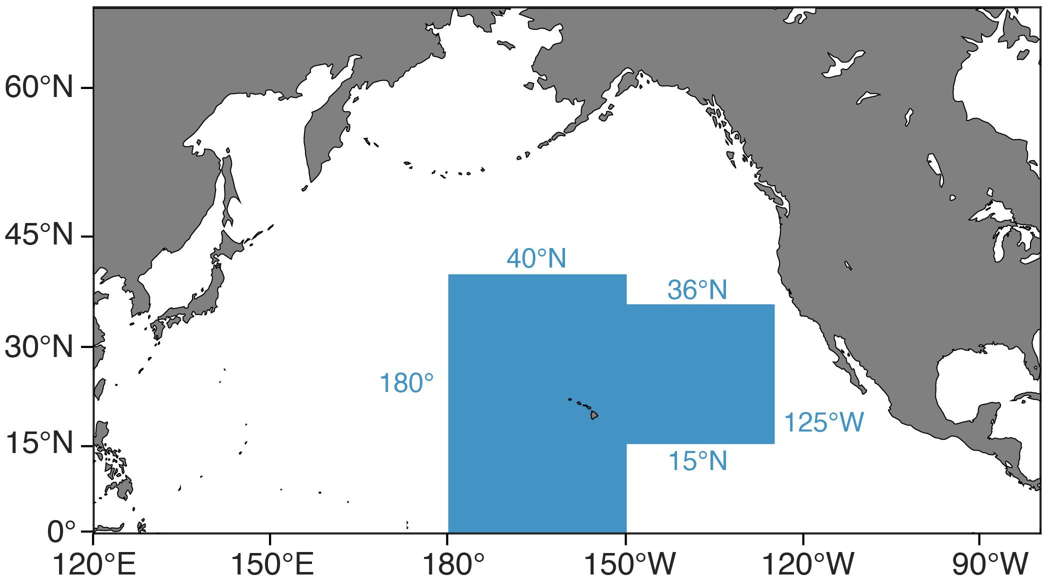
Figure 1. Map of the fishing grounds of Hawaii’s deep-set longline fishery for bigeye tuna (shaded blue).
Commercial fishing has reduced the abundance of large high-trophic level predators in this ecosystem by over 20% (Ward and Myers, 2005) and at the same time has led to increasing catch rates of smaller mesopredator species (Polovina et al., 2009). Modeling studies have replicated these historical observations using both species-based (Cox et al., 2002; Kitchell et al., 2002) and size-based (Polovina and Woodworth-Jefcoats, 2013) models. Similar modeling approaches have projected future effects of fishing and/or climate change over the 21st century. These approaches range from highly specific single species models (Lehodey et al., 2010, 2013; Del Raye and Weng, 2015) to multi-species ecosystem (Howell et al., 2013; Woodworth-Jefcoats et al., 2015) and dynamic bioclimate envelope (Cheung et al., 2010) models to size-based approaches without species-level resolution (Woodworth-Jefcoats et al., 2013, 2015; Lefort et al., 2015). Collectively, they suggest climate-driven declines in food availability may reduce fish body size (Lefort et al., 2015; Woodworth-Jefcoats et al., 2015) and biomass (Howell et al., 2013; Dueri et al., 2014; Lefort et al., 2015; Woodworth-Jefcoats et al., 2015), as well as future fishery yields (Howell et al., 2013; Woodworth-Jefcoats et al., 2015). The location of spawning and fishing grounds may also change with climate change (Cheung et al., 2010; Lehodey et al., 2010, 2013; Dueri et al., 2014; Erauskin-Extramiana et al., 2019). A number of these studies included the effects of increasing temperatures. Multi-species or species-blind approaches relied on statistical relationships (Cheung et al., 2010; Erauskin-Extramiana et al., 2019) or monotonically increasing costs of metabolism (Woodworth-Jefcoats et al., 2013), while species-specific models were able to incorporate more complex temperature effects. These include linking spawning to ocean temperature (Lehodey et al., 2010, 2013) and incorporating temperature into physiological rates (Dueri et al., 2014; Lefort et al., 2015).
Despite the array of approaches discussed above, there has not been, to our knowledge, a multi-species approach that includes both size and species resolution as well as the physiological effects of rising ocean temperatures. In this study, we use a food web model that integrates both size and species. This approach allows us to examine species-specific change in terms of biomass, abundance, and size structure. The model also incorporates temperature’s effects on metabolism as well as aerobic scope, providing more realistic future projections. Aerobic performance is closely linked to temperature (e.g., Pörtner and Peck, 2010; Pörtner, 2012) and affects fishes’ ability to forage. Our simulations include climate change’s effects on two variables which most directly affect fishes’ fitness: food supply, via changes to the plankton community, and temperature. We also examine a range of future fishing scenarios. Our results offer insight into the simultaneous effects of these stressors, and the modeling framework we developed offers a new tool for supporting strategic management decision-making in this and other regions.
Materials and Methods
Model
We developed the size-based food web model therMizer, which is a modification of mizer, a well-documented multi-species size spectrum model (Blanchard et al., 2014; Scott et al., 2014). Such models describe predation, mortality, reproduction, and physiological processes at the individual level and scale them up to population and community levels (Blanchard et al., 2017). They track the flow of biomass through fully resolved body size classes (size measured in mass) via growth and size-based predation (Blanchard et al., 2017). In mizer, the smallest fish size classes feed upon a background resource size spectrum that exhibits semi-chemostat growth dynamics (Blanchard et al., 2014; Scott et al., 2014). Our model therMizer contains two key modifications from mizer. The primary modification was incorporating the effect of ocean temperature on metabolic scope. Temperature dependencies are absent in mizer. We also replaced mizer’s semi-chemostat background resource with a resource that is input at each time step.
The effect of temperature on metabolic scope was determined by including temperature’s effect on both metabolic rate and prey encounter rate. This was incorporated into the model by scaling both rates as described below and illustrated in Figure 2. In all cases, temperature was averaged over each species’ depth range.
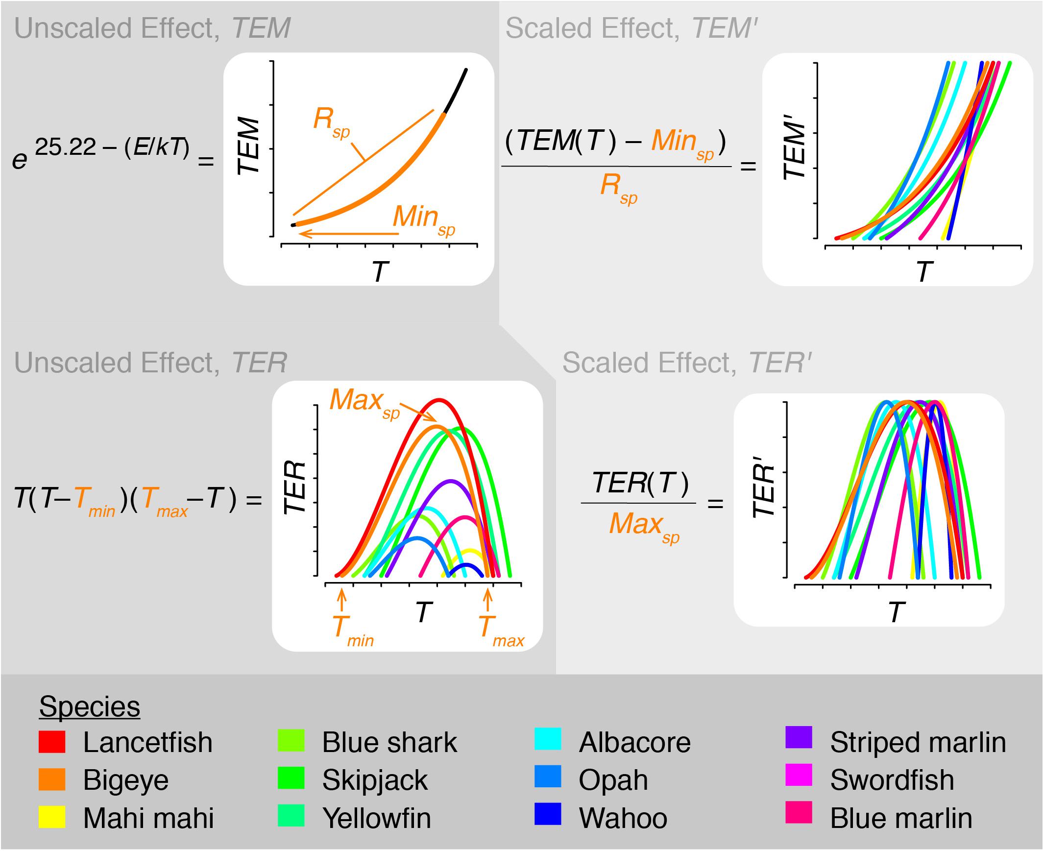
Figure 2. Schematic diagram illustrating how temperature is incorporated into therMizer. TEM, TEM′: unscaled and scaled temperature effect on metabolic rate, respectively. Rsp, Minsp: Range and minimum value of TEM, respectively, for species sp. TER, TER′: unscaled and scaled temperature effect on encounter rate, respectively. Tmin, Tmax: lower and upper limits of a given species’ thermal tolerance range. Maxsp: Maximum value of TER for species sp.
As temperature increases, metabolic rate increases. To capture this relationship, we modeled temperature’s effect on metabolic rate, TEM, following Eq. (1):
where T is vertically averaged temperature in Kelvin, k is Boltzmann’s constant (8.62 × 10⁻⁵ eV K–1), and E is activation energy (0.63 eV; Brown et al., 2004; Jennings et al., 2008). TEM was then scaled to TEM′, a value ranging from 0 to 1, following Eq. (2):
where Minsp and Rsp are the minimum value and range, respectively, of TEM for each species (Figure 2). TEM′ was then used as a multiplier for standard metabolic rate. This has the effect of standard metabolic rate being at its minimum at the lower limit of a species’ thermal range and at its maximum at the upper limit of a species’ thermal range.
In addition to influencing metabolic rate, temperature also influences aerobic scope and fishes’ ability to successfully forage. To capture this relationship, we incorporated temperature into prey encounter rate. While species-specific thermal performance parameters are largely lacking in the literature, the relationship between temperature and aerobic scope is broadly understood (Pörtner and Peck, 2010). Therefore, we modeled the effect of temperature on encounter rate, TER, using a generic polynomial rate equation (van der Heide et al., 2006):
where T is vertically averaged temperature, Tmin is a species’ minimum thermal tolerance, and Tmax is a species’ maximum thermal tolerance (Figure 2). All temperatures in Eq. (3) are in °C. TER was then scaled to TER′, a value ranging from 0 to 1, by dividing by Maxsp, the maximum value of TER for each species (Figure 2). TER′ was then used as a multiplier for encounter rate. This has the effect of species being able to realize peak aerobic performance and encounter the maximum amount of prey possible when they are at their optimal temperature. Foraging success declines to either side of this temperature.
The joint effects of temperature on metabolic rate and prey encounter rate (TEM′ and TER′, respectively) are shown in Figure 3. At temperatures outside species’ thermal range, both TEM′ and TER′ were set to 0 representing local extinction. Species’ thermal and vertical ranges are listed in Table 1.
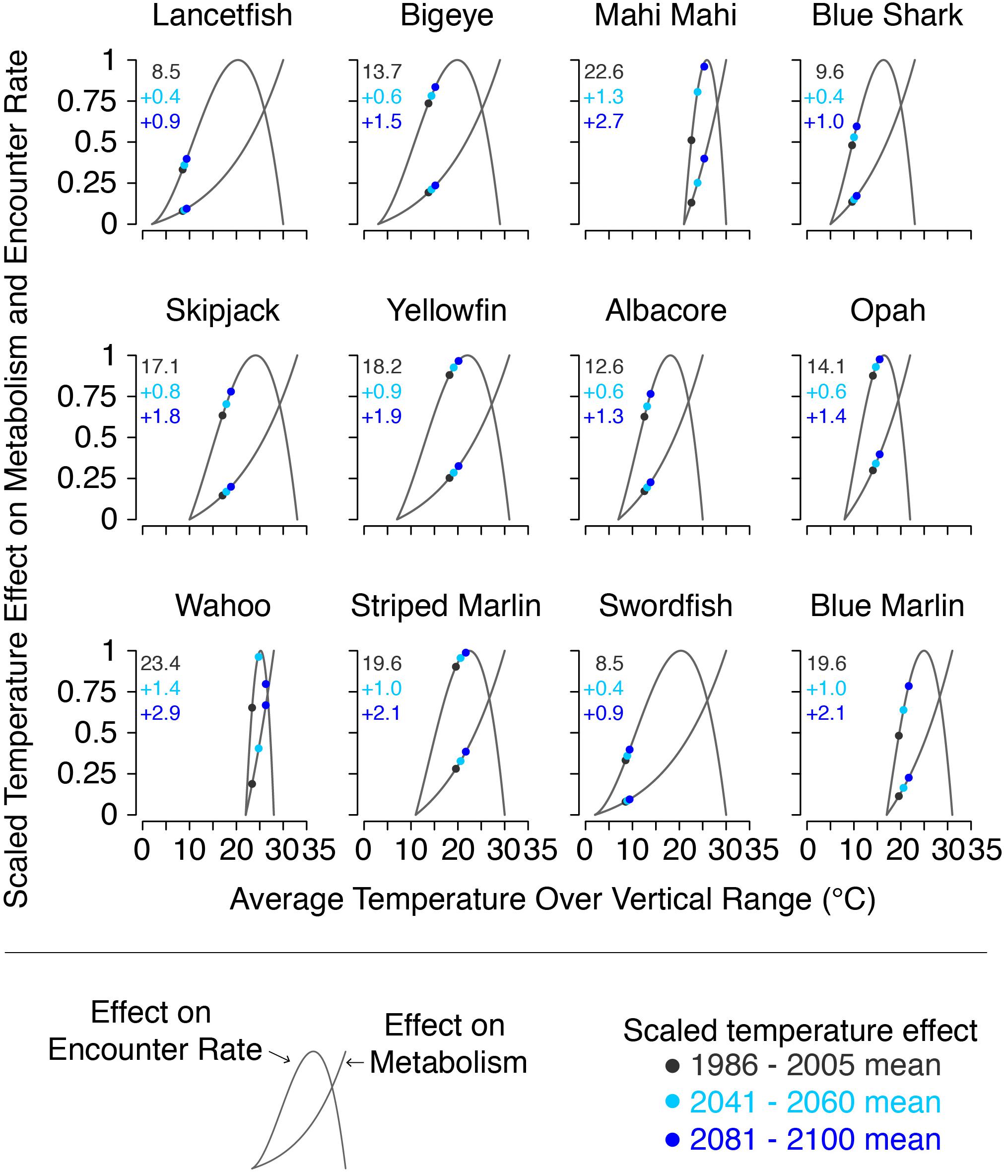
Figure 3. Scaled thermal effects on metabolic and encounter rates for each species at the beginning, middle, and end of the 21st century, along with the mean temperature at the beginning of the century (black text), and its projected change by the middle and end of the century (blue text). Values plotted are the multi-model mean from the CMIP5 models used in this study. Gray lines show the full range of values possible for each species.
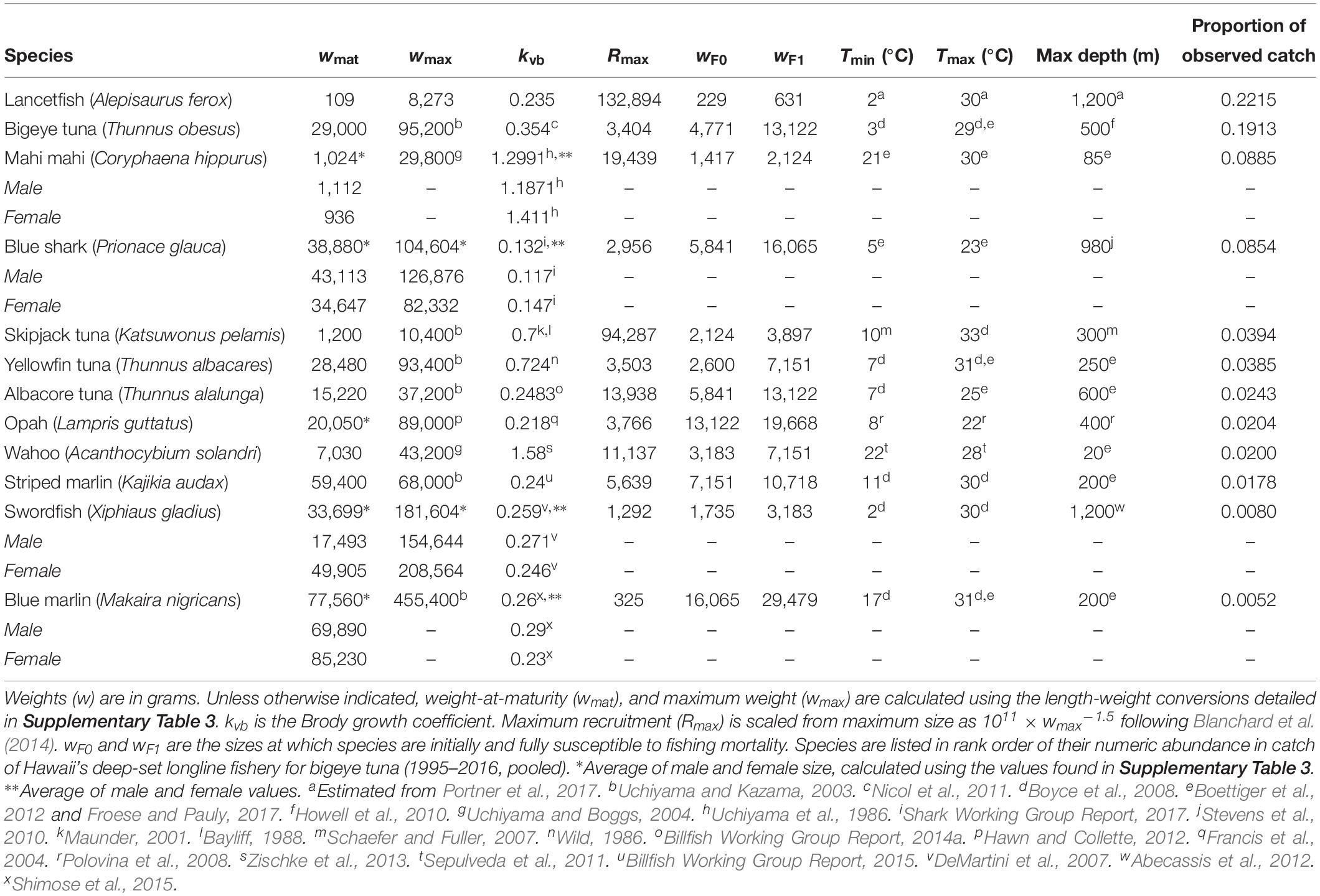
Table 1. Species-specific model parameters.
Model Parameters and Input
We attempted to include as many species as possible of the top 20 species caught by the Hawaii deep-set longline fishery, regardless of species’ commercial value. The 12 species listed in Table 1 are those for which there was sufficient life history and thermal tolerance information available to parameterize the model. Together, these species account for 76% of the fishery’s observed catch.
Parameters and Calibration
Global model parameters were left unchanged from the default mizer settings (Blanchard et al., 2014; Scott et al., 2014), with the exception of kappa (κ) which we set at 1012. This variable is used in determining species’ initial size spectra (Blanchard et al., 2014). Also as in Blanchard et al. (2014), all teleosts enter the model as larvae weighing 1 mg. Blue sharks enter at 354 g, an average of mean male and female birth weights (344 and 362 g, respectively; Shark Working Group Report, 2017). The additional species-specific parameters are listed in Table 1. Values in Table 1 were taken from the literature as noted, with the exception of the Brody growth coefficient, kvb, for lancetfish. Estimates of this parameter for lancetfish were not available in the literature. Based on available values for similar species (Morales-Nin and Sena-Carvalho, 1996; Lorenzo and Pajuelo, 1999; Harada and Ozawa, 2003; Figueiredo et al., 2015; Froese and Pauly, 2017), we used the median value of the lower quartile of teleost kvb values.
Predation in therMizer is both species- and size- specific. All fish have a log-normal prey size preference that is dependent upon predator body size, species’ predator-prey mass ratio (100 for teleosts, Blanchard et al., 2014; 400 for blue sharks, Barnes et al., 2008), and the width of the prey selection window (1 for all species, Blanchard et al., 2014). Prey selection is further informed by the interaction matrix (Supplementary Table 1). Interaction, θij, between species i and j ranges from 0 to 1. Previous size spectrum models have determined the interaction matrix values based on horizontal overlap as inferred from bottom trawl surveys (Blanchard et al., 2014; Reum et al., 2019). Here, we determined interaction based on species’ vertical overlap following Eqs (4) and (5) and illustrated in Figure 4:
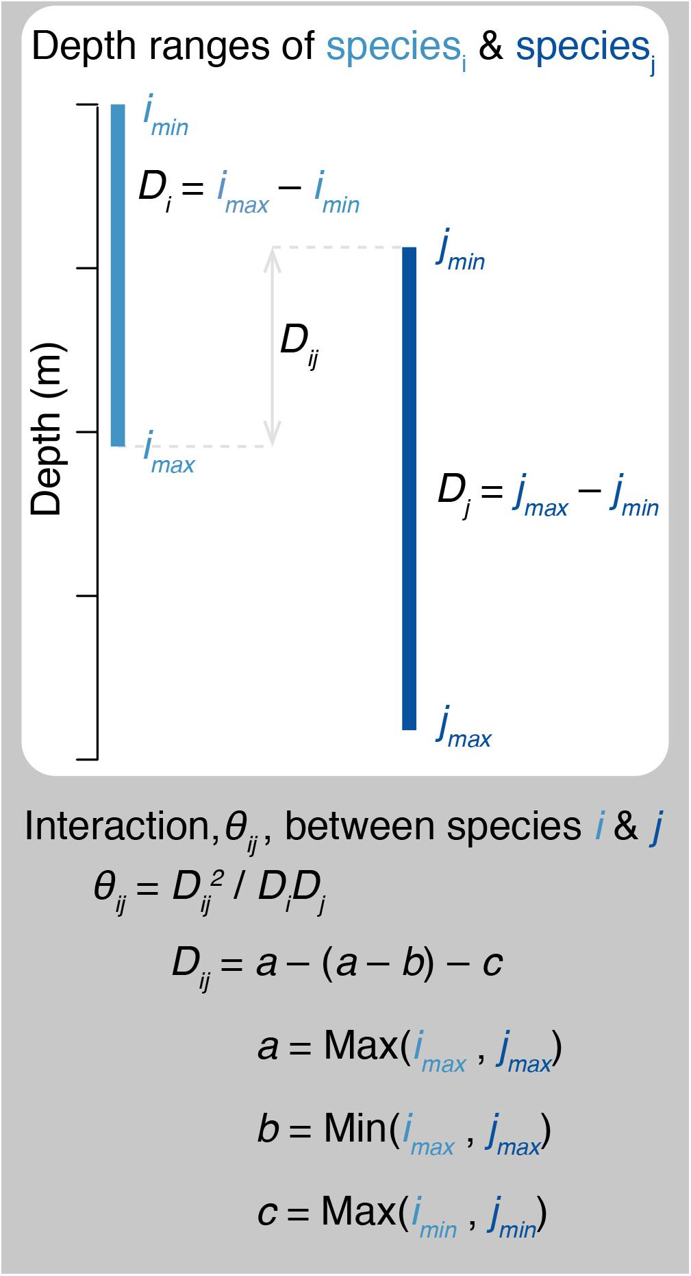
Figure 4. Schematic diagram illustrating how predator – prey interactions are calculated. θij, interaction between species i and j. Di, Dj, depth ranges of species i and j, as determined from species’ minimum and maximum depths (e.g., imin and imax). Dij, range of overlapping depths for species i and j.
where Di and Dj are the depth ranges of species i and j, respectively; Dij is the range of overlapping depths for species i and j; and a is the greater maximum depth, b is the lesser maximum depth, and c is the greater minimum depth for the pair of species i and j. All species have a minimum depth of 0 m, with the exception of opah which has a minimum depth of 50 m (Polovina et al., 2008). For all species pairs, the interaction matrix determines the proportion of total prey biomass of the appropriate size that is available to the predator.
Fishing mortality increases linearly from 0 to F over a size range unique to each species. Fishing mortality is phased in over a range of body sizes to account for longline gear’s inefficiency in catching smaller body sizes (Polovina and Woodworth-Jefcoats, 2013). To establish these sizes, we used time-averaged (2006–2016, pooled) catch records from the Pacific Islands Region Observer Program, which since 2006 has recorded the size of every third fish caught by Hawaii’s longline bigeye tuna fleet. Roughly 20% of this fishery’s effort is observed, and observer records have been found to correlate well with vessel logbooks (Woodworth-Jefcoats et al., 2018). We binned observed sizes of fish caught into equally spaced logarithmic size classes as in therMizer (Scott et al., 2014; Edwards et al., 2017). Each species is initially susceptible to fishing mortality at the size which contributes at least 1% toward that species’ total observed catch. Fish are fully susceptible to fishing mortality at the size which contributed the most to that species’ total catch. The sizes at which each species is first and then fully susceptible to fishing mortality are listed in Table 1.
Climate Forcing Variables
We used output from a suite of earth system models included in the 5th phase of the Coupled Model Intercomparison Project (CMIP5; Taylor et al., 2012; Supplementary Table 2). CMIP is a coordinated international climate and earth system modeling approach that centers around common model forcings and output variables (Taylor et al., 2012). Phyto- and zooplankton densities (Figure 5) were vertically integrated over the upper 200 m of the water column. Numerical abundance within each size class was determined by dividing density by mean size. Plankton size spectra were created as linear fits to log-transformed abundances and sizes. Model-specific plankton size classes are listed in Supplementary Table 2.
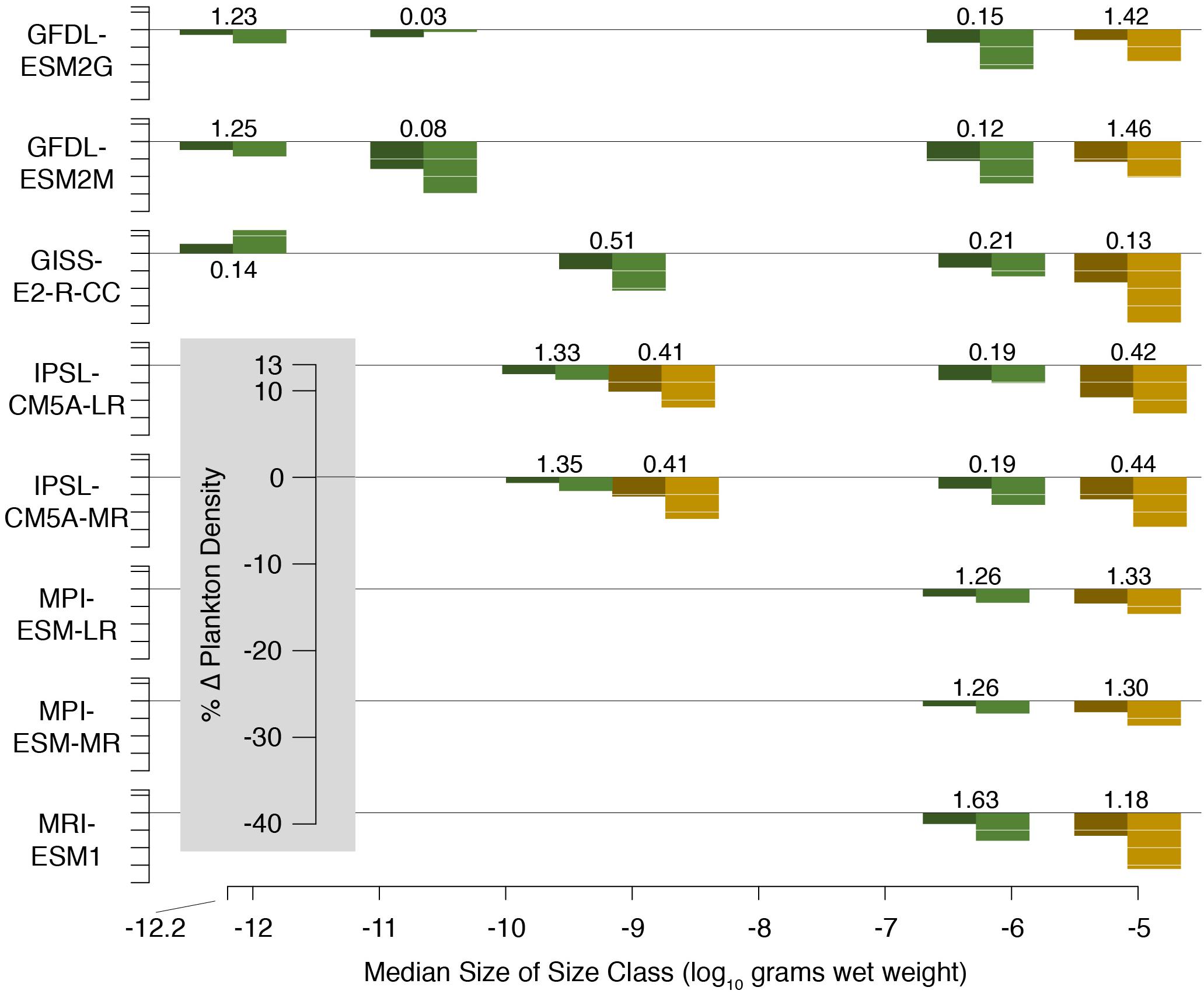
Figure 5. Change in phyto- (green) and zooplankton (brown) densities projected by CMIP5 models by the middle (dark shading) and end (light shading) of the 21st century. Change is relative to the average of the last 20 years of the historical run (1986–2005) which is listed adjacent to each set of bars. Initial plankton biomass densities are in units of g C m–2.
As with the original mizer model, some calibration of the background resource was required (Blanchard et al., 2014). To this end, we compared the above described plankton spectra with the background spectrum generated by the semi-chemostat resource model to determine appropriate scaling for the slope (×1.2) and intercept (×0.8) of the CMIP5-generated plankton spectra. These scaled spectra were extended to therMizer’s full size range to determine the background resource at each time step. Initial spectra for individual fish species were determined as in the original mizer model (Scott et al., 2014).
Ocean temperature for each species was determined by averaging across each species’ depth range. Initial temperatures are from World Ocean Atlas 2013 v2 data (Locarnini et al., 2013). Temperature changes from the CMIP5 models were then applied to these initial temperatures. This approach accounts for potential bias in the CMIP5 models.
Model input plankton densities are summed and temperatures averaged over the footprint of the Hawaii-based deep-set longline fishery targeting bigeye tuna: 0°–40°N from 180°–150°W and 15°–36°N from 150°–125°W (Figure 1; Woodworth-Jefcoats et al., 2018). Across the CMIP5 models used, phytoplankton densities declined by an average of 6% by mid-century and 12% by 2100. Declines in zooplankton density were twice that of phytoplankton, i.e., 12% by mid-century and 24% by 2100 (Figure 5). All species, regardless of vertical range, were projected to encounter rising ocean temperatures (Figure 3). For the deepest-living species modeled which have a maximum depth of over 1000 m, temperatures increased by about 0.5°C by mid-century and 1°C by 2100. For the shallowest-living species which live within 100 m of the ocean’s surface, temperatures increased by nearly three-times this amount or roughly 1.5°C by 2050 and 3°C by 2100.
Model Verification
Model output from a run forced with a static climate (1986–2005 mean) and constant fishing mortality (F = 0.2) was compared to time-averaged records of observed catch (see description of the observer data above). Observed sizes were binned as in therMizer to create size spectra of catch. Modeled and observed catch size spectra were well correlated, with Pearson’s correlation coefficient, r, ranging from 0.39 to 0.85 (Supplementary Figure 1). We used a value of F = 0.2 for model verification because, for the species for which there are stock assessments, most of these assessments estimate fishing mortality to be close to this value (e.g., Billfish Working Group Report, 2014a, b, 2016; McKenchie et al., 2017; Shark Working Group Report, 2017; Xu et al., 2018).
Scenarios Modeled
We evaluated the individual and joint effects of climate change and fishing on the ecosystem and on fishery catch. In all scenarios, the model was run for 600 years with a static climate (1986–2005 mean) and constant fishing mortality (F = 0.2) to account for spin-up effects and allow the model to reach equilibrium. Projections run from 2006 through 2100. To assess the impact of climate change alone, we held fishing mortality constant at F = 0.2. To assess the impact of fishing alone, we used a static climate scenario. In all cases where a variable was held static, we held the spin-up value constant over the 21st century.
We examined four scenarios in which fishing mortality changed linearly over the projection period (2006–2100): doubling from F = 0.2 to 0.4, increasing five-fold to 1, halving to 0.1, and declining to one fifth or 0.04 (hereafter referred to as 2F, 5F, 0.5F, and 0.2F, respectively). These scenarios were chosen based in part on trends in effort of Hawaii’s deep-set longline fishery. Over the logbook record, effort has risen more than five-fold from 8.4 million hooks set in 1995 to over 47 million hooks set in 2015 (Woodworth-Jefcoats et al., 2018). Fishing effort does not translate equally to fishing mortality, and therefore we consider 5F to be a fairly aggressive future fishing scenario. We also considered the effect of fishing mortality doubling (2F) as a more moderate scenario. We simply used the reciprocals of the fishing increase scenarios to model a decline in fishing mortality. This facilitated scenario comparison. To further facilitate scenario comparison, we used the same value of F for all species. This approach eliminated potential confounding influences of fishing different species at different levels of intensity and replicated observed catch reasonably well (see section “Model Verification” above). However, we note that therMizer is capable of incorporating species-specific F values (Scott et al., 2014).
We evaluated several measures of ecosystem structure and fishery performance. Total biomass and abundance provide species-specific measures of the fishery’s catch and its relation to the ecosystem. We refer to ecosystem biomass as “biomass” and catch in weight as “yield.” The large fish indicator (LFI; Blanchard et al., 2014) is a broad measure of the numerical proportion of fish ≥15 kg (Polovina and Woodworth-Jefcoats, 2013; Woodworth-Jefcoats et al., 2015). The LFI provides insight into both the size structure of the ecosystem as well as the potential value of fish catch, as larger fish are generally more valuable. As a complementary measure to the LFI, we also examined the change in species’ mean size.
We assessed these measures both through time series over the projection period as well as with 20-year averages in an effort to minimize the confounding influence of interannual variability. We averaged results over three 20-year time periods to capture the beginning, middle, and end of the 21st century: 1986–2005, 2041–2060, and 2081–2100 (hereafter referred to as 2000, 2050, and 2100, respectively). The 1986–2005 average corresponds to the equilibrium value at the start of the therMizer projections.
Results
We find that, taken as individual stressors, climate change and increasing fishing mortality act to reduce fish biomass and size across all species. The effects of reduced fishing mortality are generally of the opposite sign. However, when modeled jointly, there were no scenarios in which yield increased. Results for the ecosystem supporting the fishery are slightly more optimistic, with reduced fishing mortality somewhat offsetting the negative effects of climate change.
Total Biomass and Yield
Climate change, with constant F, acts to reduce bigeye biomass by 7% by 2050 and by 20% by 2100. Across all species modeled, these declines range from 3% (skipjack) to 14% (blue shark) by 2050 and from 7% (skipjack) to 37% (wahoo) percent by 2100. Declines in yield reflect declines in ecosystem biomass (Figure 6).
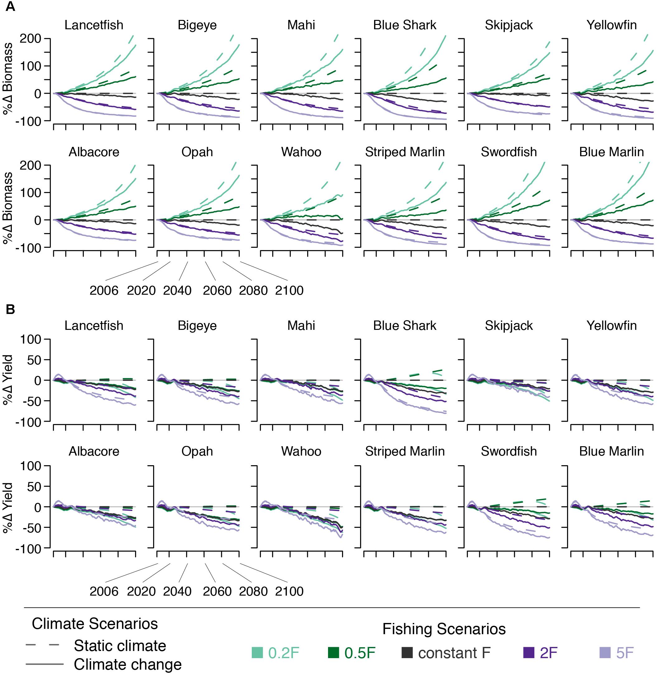
Figure 6. Percent change in species’ (A) biomass and (B) yield under five fishing scenarios (indicated by line color) both with (solid lines) and without (dashed lines) climate change.
For all species, in the absence of climate change, decreasing F leads to increasing biomass, and vice versa. This is because lower levels of F result in less biomass being removed as yield. Both scenarios with increasing F lead to declining yield for all species, due to declining biomass. Likewise, the 0.2F scenario also leads to declining yield, due to less fishing effort, for all but the largest species (swordfish, blue shark, and blue marlin). The yield of these three largest species increases an average of 7% by 2050 and 8% by 2100 (Figure 6). The 0.5F scenario leads to similarly little change in yield by 2050 (<10% change). By 2100, roughly half the species modeled see an increase in yield of 25% or less, while two see no change, and three see small (<10%) declines (Figure 6).
We find that when changes in F are paired with climate change, reducing F can compensate somewhat the climate-driven biomass declines for all species. Bigeye biomass increases to within 10–12% of what it would be in the absence of climate change by 2050 under the 0.5F + climate change and 0.2F + climate change scenarios. Across all species, this value ranges from 4 to 23% (Figure 6). By 2100, biomass of all species except wahoo more than doubles (bigeye biomass increases 136%) when climate change is incorporated into the 0.2F scenario. When climate change is included in the 5F scenario, yield increases over the initial ∼15 years and then declines. Other than this short-term increase, there is a decline in yield for all species under all fishing scenarios; none of the modeled fishing scenarios were able to compensate for the climate-driven declines in yield. Furthermore, climate change amplified the biomass declines seen under scenarios with increasing fishing mortality.
Total Abundance
Climate change, in the absence of changing F, increases the abundance of a number of species (Figure 7). By 2050, all species except blue shark experience an increase in abundance of 1–9%. By 2100, all species except blue shark, yellowfin, wahoo, striped marlin, and swordfish experience increases in abundance of 1–17%. Blue shark abundance declines by 10 and 21% across these time points. Yellowfin, wahoo, and striped marlin abundance decline by 9, 9, and 10%, respectively. Swordfish abundance is unchanged by 2100, despite increasing earlier in the century (Figure 7).
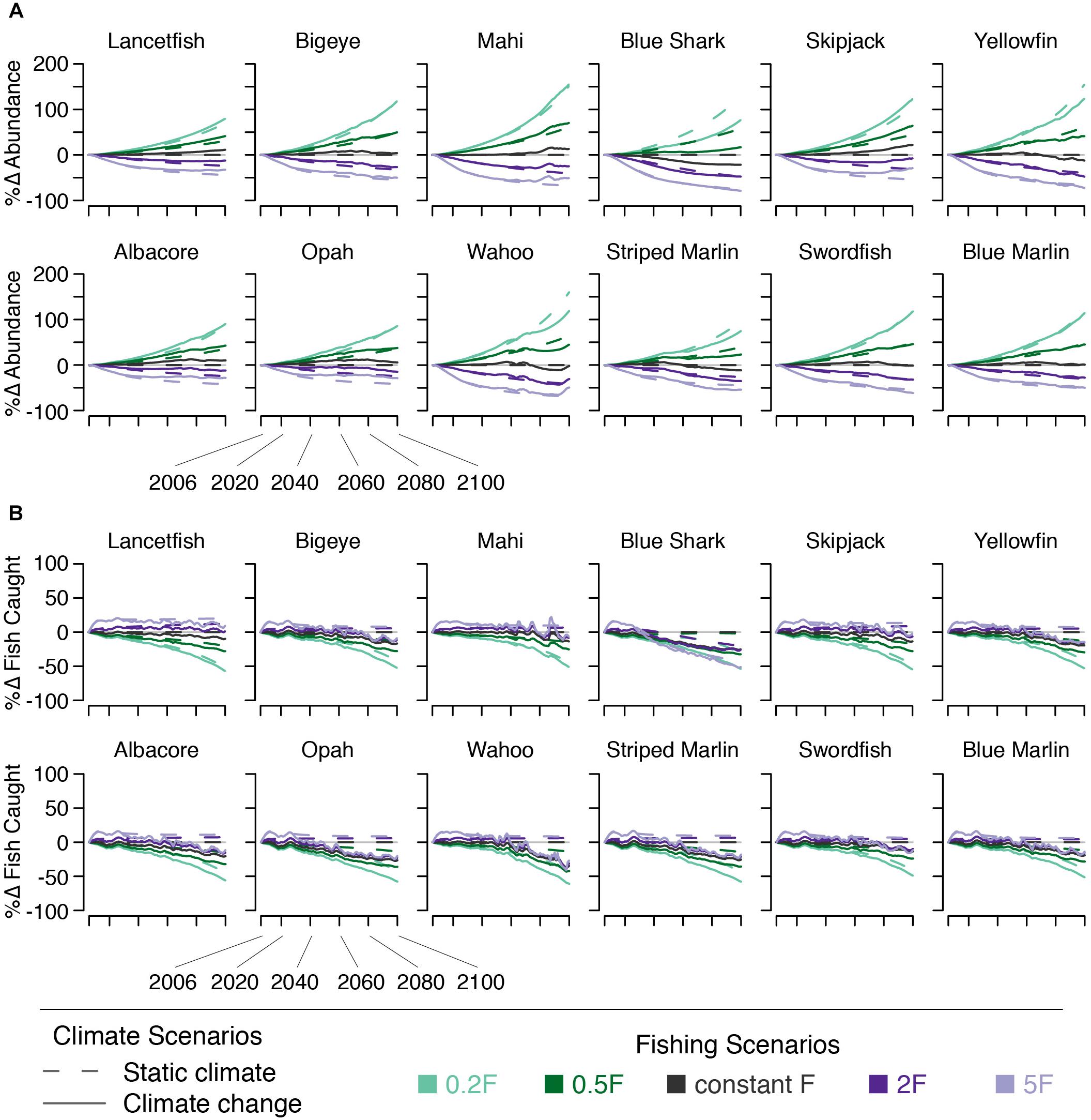
Figure 7. Percent change in (A) species’ numerical abundance and (B) number of fish caught under five fishing scenarios (indicated by line color) both with (solid lines) and without (dashed lines) climate change.
The effects of changing F on abundance are essentially the same as those on biomass: declining fishing mortality leads to increased fish abundance and vice versa. The effects on the number of fish caught, however, are different than those of biomass (i.e., decreasing fishing mortality leads to a decline in the number of fish caught, Figure 7).
The effects on abundance of pairing climate change and changes in F varied by species. For species that saw abundance increase under climate change, the climate effect somewhat dampened the abundance declines resulting from increasing F and amplified increases in abundance under decreasing F. For species that saw abundance decline under climate change, these declines were exacerbated by increasing F. When F was reduced, climate change dampened the expected increases in abundance (Figure 7).
Large Fish Indicator
The effect of climate change on the large fish indicator (LFI) was small in the absence of changing F. LFI declines from 0.129 to 0.119 by 2050 and to 0.105 by 2100. Catch LFI declines as well, falling from 0.218 to 0.201 by 2050 and to 0.173 by 2100 (Figure 8).
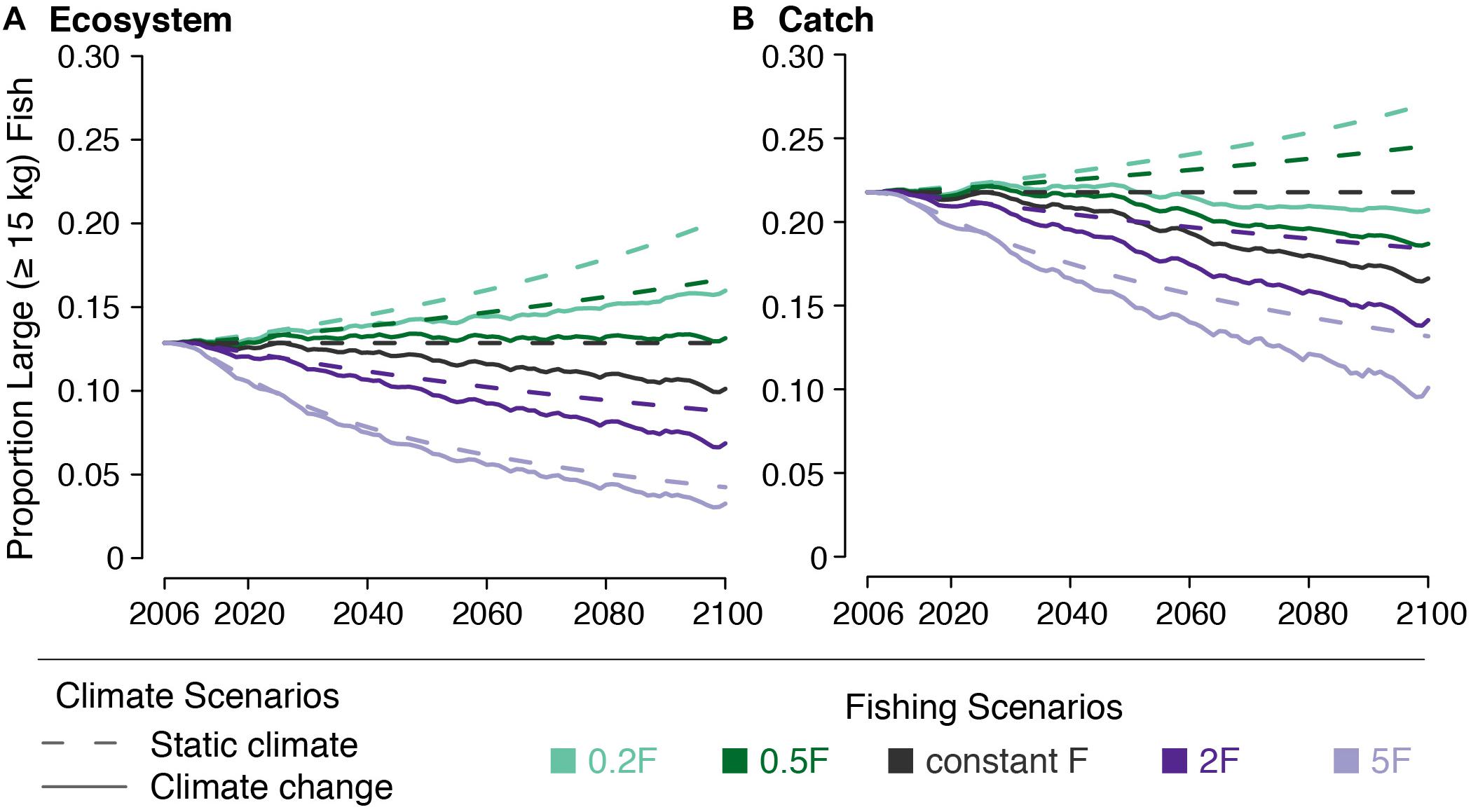
Figure 8. Large fish indicator (LFI) for (A) the ecosystem and (B) the catch under five fishing scenarios (indicated by line color) both with (solid lines) and without (dashed lines) climate change.
The effects of changing F on LFI were greater than those from climate change. Reducing F led to LFI increasing from 0.129 in 2000 to 0.143–0.162 by 2050 and to 0.153–0.191 by 2100, across both the 0.5F and 0.2F scenarios. Increasing F had a greater effect on LFI, reducing it to 0.069–0.107 by 2050 and to 0.046–0.091 by 2100, across both the 2F and 5F scenarios. The effects on catch LFI were similar (Figure 8).
We found that when paired with climate change, halving F almost equally offset the decreased LFI caused by climate change alone (Figure 8). Climate change acted to undermine the increase in LFI caused by decreasing F to one fifth the initial value. Climate change also exacerbated the decline in LFI caused by increasing F. When looking at modeled catch, we found that neither modeled decrease in F was able to offset the decline in LFI after 2050. By 2100, catch LFI declined to 0.208 under the 0.2F + climate change scenario and to 0.109 under the 5F + climate change scenario.
Mean Size
Mean size declined for all species under climate change alone. By 2050, declines in mean size range from 4% (blue shark) to 13% (yellowfin, wahoo, striped marlin, and swordfish) across species, with bigeye mean size declining by 11%. By 2100, mean size declines by 8–38% across species, with blue shark experiencing the least and wahoo experiencing the greatest decline in mean size (bigeye declines by 23%). Declines in the mean size of fish caught are slightly smaller (Figure 9).
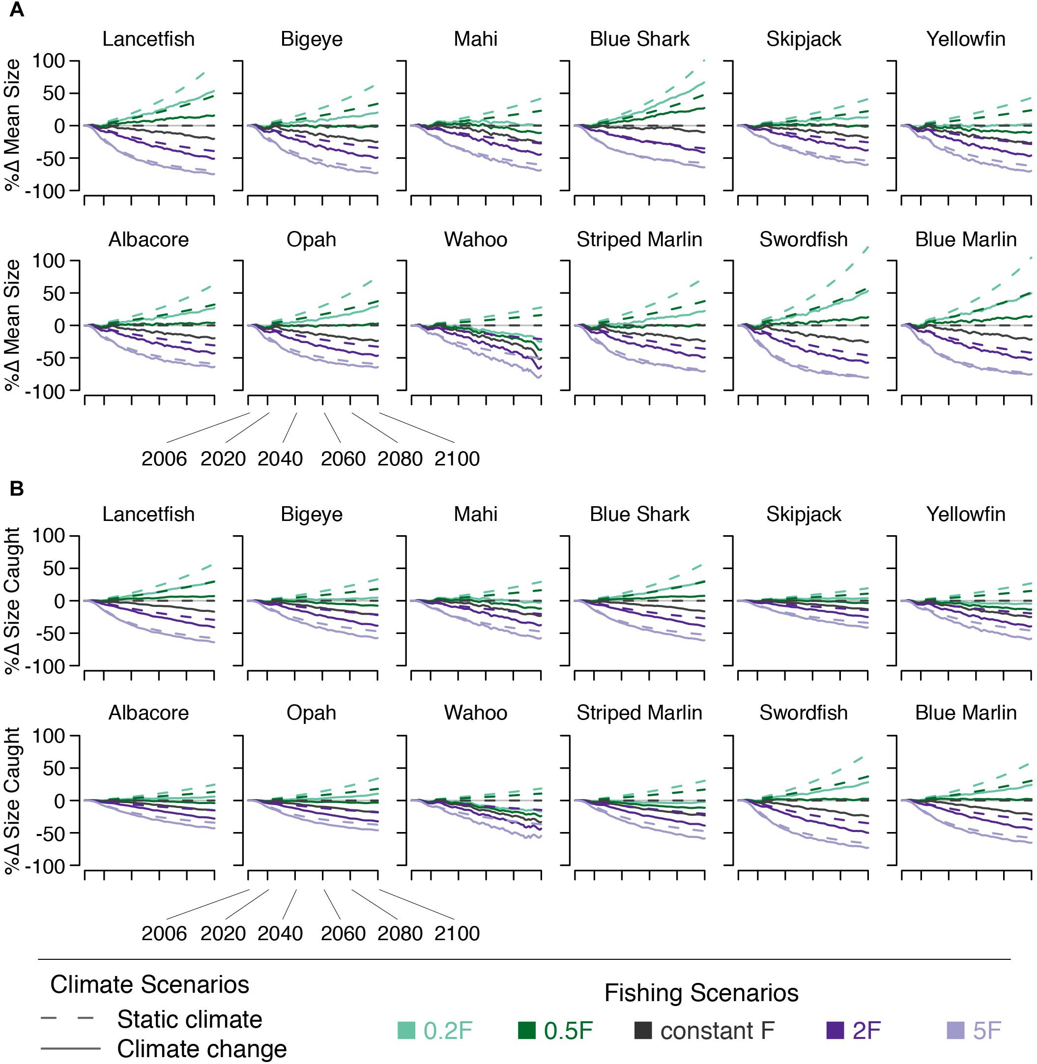
Figure 9. Percent change in (A) species’ mean size and (B) the mean size of fish caught under five fishing scenarios (indicated by line color) both with (solid lines) and without (dashed lines) climate change.
Because fishing targets a species’ largest body sizes, the effects on mean size of changing F are fairly straightforward: In the absence of climate change increasing F leads to mean body sizes decreasing by 11–62% by 2050 across both the 2F and 5F scenarios, with bigeye size decreasing by 19–48% across these scenarios. By 2100, increasing F leads to mean body size decreasing by 19–77% (bigeye by 32–64%). Decreasing F has the opposite effect on mean size. By 2050, the increase is somewhat less than opposite that of the reciprocal fishing scenario. However, by 2100, reciprocal fishing scenarios result in nearly opposite effects on mean size. As with other indicators, these effects are somewhat dampened in the catch relative to the ecosystem due to the size-selective nature of fishing (Figure 9).
The joint effect of fishing and climate change on species’ mean size varied by species. Reduced F was able to offset the climate-induced decline in mean size, to some degree, for all species. By 2100, the 0.2F + climate change scenario led to increases in mean size for all species except wahoo. The 0.5F + climate change scenario allowed mean size to increase for roughly half the species modeled. These results were dampened in the modeled catch. By 2050, the mean size of fish caught changed by −8–+11% across species under the 0.5F + climate change and 0.2F + climate change scenarios. The change in size of bigeye caught in 2050 ranged from −2–+2% across these two scenarios. By 2100, the 0.5F + climate change scenario allowed mean size of fish caught to increase in four species (lancetfish, blue shark, swordfish, and blue marlin). The 0.2F + climate change scenario allowed mean size caught to increase in all but four species (mahi, yellowfin, wahoo, and striped marlin; Figure 9).
Discussion
We used therMizer, a size-structured food web model with individual species that is capable of capturing the metabolic effects of rising ocean temperatures, to assess the effects of climate change and fishing on Hawaii’s deep-set longline fishery and its supporting ecosystem. Our results show that while a decline in this fishery’s yield seems likely, this may mask resilience in the ecosystem supporting the fishery. The contrast between changes in catch and changes to the ecosystem is particularly noteworthy as it highlights the limited ability of some fishery dependent data to fully capture ecosystem trends.
Outlook for Future Yield and Ecosystem
Our results show that as the climate continues to change, a decline in the yield of Hawaii’s bigeye tuna fishery seems inevitable. None of the changes in fishing mortality that we modeled, whether increasing or decreasing, allowed yield to increase after more than about 15 years. These results reinforce those of Howell et al. (2013), who found that climate change is projected to reduce the Hawaii longline fishery’s target yield even when fishing mortality is halved. Their study used an Ecopath with Ecosim model to simulate food web and fishery response to climate change. That two dissimilar modeling methods produce similar projections for declining yield should be noted by regional fishery managers. Additional modeling (e.g., Cheung et al., 2016; Fu et al., 2018; Queirós et al., 2018) and empirical (Watson et al., 2012) studies of other ecosystems have led to similar projections.
In addition to total yield declining, we also find that the proportion of large fish in the catch declines in all scenarios after 2050. This suggests that not only will yield be reduced, but all else being equal, the fish caught may be less valuable because there will be fewer large fish. That said, increasing fishing mortality does lead to increased numbers of fish caught for some species (Figure 7). This is likely because therMizer models fishing mortality as a removal of a numeric percentage rather than a biomass percentage (i.e., as F increases, a greater number of individuals is removed, though yield may still decline if those individuals’ mean size declines).
Despite the poor outlook for fishery yield, we find that the ecosystem may be more resilient under specific future scenarios. Biomass of all species increases when climate change is modeled jointly with a reduction in fishing effort (Figure 6). This result reinforces calls from previous authors that reduced fishing can help reduce the effects of climate change (e.g., Brander, 2013). We also find that halving fishing mortality allows the LFI to remain essentially unchanged over the 21st century, and that reducing fishing mortality to one fifth initial values allows the LFI to increase. Ultimately, the decision of whether to lower fishing mortality in favor of ecosystem resilience comes down to societal values. Models such as therMizer can help fishery managers and other stakeholders understand a broad range of fishery management consequences (Blanchard et al., 2014; Cheung et al., 2016).
Mechanisms Driving Change
One value in modeling studies is that they allow for investigation of the mechanisms driving change. This is particularly valuable when different stressors have the same effect; without being able to examine the underlying mechanisms it can be easy to assume that they are the same. We find that both climate change and increasing fishing mortality have similar effects on the central North Pacific’s ecosystem and fishery yield: reduced biomass and a decline in mean body size. However, the mechanisms driving this response are different. The declining plankton biomass projected as a result of climate change reduces the amount of energy (food) available to all predators. This leads to reduced growth and, in turn, lower biomass. The shift in the plankton community’s size structure also propagates through the food web, with proportionally less food available to larger body sizes, further reducing growth at larger body sizes. This disproportionate allocation of limited resources shifts the size structure toward smaller body sizes, resulting in a decline in mean body size across species (see also the discussion of species-specific effects below). Further, the disproportionate allocation of resources favoring smaller body sizes, paired with the inverse relationship between abundance and body size, explains why climate change leads to increased numerical abundance for some species.
Fishing, on the other hand, selectively removes the largest individuals from the population. Because a single large individual can be orders of magnitude larger than smaller individuals, removal of numerous large fish reduces both total biomass and mean size. Conversely, allowing more large individuals to remain in the ecosystem by reducing fishing effort more than counteracts the effect of removing them (Figures 6, 9).
Modeling climate change and fishing jointly highlights the different mechanism at work to drive ecosystem change. Regardless of how fishing mortality changes, climate change acts to lower the system’s carrying capacity, thereby reducing potential biomass, abundance, and yield. This interaction of stressors is only apparent when they’re modeled together. Such interaction may explain the diminished impact of climate change as fishing mortality increases. As fishing increases, its effects may overshadow the lower carrying capacity resulting from climate change (Blanchard et al., 2012). This result is somewhat surprising given that a number of studies have found that the effects of climate change are stronger on more heavily fished systems (e.g., Blanchard et al., 2012; Brander, 2013). One possible explanation for this disparity may be tied to model structure (Woodworth-Jefcoats et al., 2015). Application of mizer to another ecosystem produced results similar to ours. Fu et al. (2018) found that higher trophic level fish were more likely than those at lower trophic levels to see dampened effects when fishing and climate change were combined. The species considered in our study are nearly all high trophic level species. We encourage further ecosystem modeling comparisons across modeling frameworks and ecosystems to help separate model structure from ecosystem structure (e.g., Tittensor et al., 2018). We also encourage further studies to consider the joint effects of stressors, especially in the open ocean beyond the limits of EEZs and LMEs given the relative paucity of studies doing so (Ortuño Crespo and Dunn, 2017).
Another mechanism that we investigate in this study is the role that temperature plays in driving species’ response to climate change. We find that shallower-living species, most notably wahoo, see the greatest effect from climate change. On the other hand, species projected to see the least warming (e.g., lancetfish, swordfish, and blue shark) experience an increase in mean body size under both scenarios where decreasing fishing mortality is paired with climate change. Rising temperatures exacerbate the effect of reduced food availability by both increasing metabolic demand and reducing aerobic scope. This means that as climate change progresses fish will need more food despite there being less available, and that they’ll be less able to successfully forage for this food. The large effect that rising temperature has on wahoo and, to some degree, on mahi mahi, suggests that shallower-living species may be bellwethers of larger ecosystem changes. It also creates the potential for a shifting species composition of both the ecosystem and catch as species are differentially affected by rising ocean temperatures. Conducting additional therMizer simulations with more spatially discrete temperature projections, both vertically and horizontally, or with temperature exposure varying across life stages could provide further insight into how species may be affected by the ocean’s warming.
Our method for incorporating temperature’s effect on metabolic demand and aerobic scope requires only minimal parameterization (universal constants and species’ thermal tolerance limits). This potentially increases the utility of the approach across other modeling frameworks. Similarly, it could provide an independent first approximation of how individual marine species may be affected by climate change. Others have highlighted the need to better incorporate aerobic scope into projections of climate effects (e.g., Pörtner, 2012). If a similarly simple approach could be applied to the relationship between oxygen or carbon dioxide and aerobic scope, this would significantly enhance our abilities to meet this challenge.
Food web interactions are also an integral mechanism in the response to fishing and climate change. We find that the impact of warming is somewhat offset by the effect of body size on predation. For example, blue marlin, the largest species in our simulations, experiences an increase in mean size when climate change is paired with decreasing fishing mortality, despite being a fairly shallow-living species (Table 1). This is likely due to the lack of competition between blue marlin and other species for prey, as its maximum body size exceeds those of other species (Kitchell et al., 2002). Conversely, yellowfin tuna, which has a maximum body size nearly one-fifth that of blue marlin sees its mean size decrease or remain constant under these scenarios despite having a deeper vertical range. This might be a result of yellowfin tuna being both predator and prey simultaneously (Cox et al., 2002; Kitchell et al., 2006). We note also that food web interactions would perhaps be more important in scenarios where different species are subject to different levels of fishing mortality, as they are in real systems. In this case, food web interactions could act to amplify or dampen fishing effects or the effects of climate change.
Sources of Uncertainty
Three primary sources of uncertainty emerged in this study. The first is linked to the range of the CMIP5 models’ plankton densities. While there is broad agreement across CMIP5 models regarding change in temperature, these models vary substantially in their values for plankton densities (Figure 5; Woodworth-Jefcoats et al., 2017). We’ve presented the multi-model mean across CMIP5 models in this study for clarity. However, the range of plankton values and change in plankton values leads to quite a wide range in therMizer output forced by different CMIP5 models. To some degree, this is expected as CMIP5 was the first CMIP to include zooplankton among the output variables. Skill will likely improve in future generations of earth system models and CMIP6 has intercomparisons planned toward this goal (Eyring et al., 2016). We note, though, that a reliable baseline to which modeled changes could be applied (which is how temperature is treated in this study) would be valuable to future earth system and ecosystem modeling efforts. It could also help reconcile differences in the magnitude of observed and modeled size spectra (Supplementary Figure 1). Such an empirical baseline exists for physical oceanographic variables in the World Ocean Atlas. While there are global plankton databases (e.g., COPEPOD; O’Brien, 2010), their coverage is fairly limited.
The second major source of uncertainty is the species-specific model parameters. For example, the effect of rising temperature depends in part on where thermal habitat places species’ metabolic scope (Rountrey et al., 2014). For species with narrow thermal ranges (e.g., wahoo), a small change in temperature can have a large impact on metabolic scope. We note that our modeled metabolic scope is dependent on the accuracy of species’ thermal tolerance limits. For well-studied fish such as tuna, these tolerance limits are likely accurate. However, for other species, particularly those of no commercial value, these tolerance limits are inferred from data such as diet or vertical range. Better understanding of how species use their full three-dimensional habitat would reduce model uncertainty.
Uncertainty around other species-specific parameters such as maximum recruitment, growth rate, and size-at-maturity also likely influences the model’s results. A mizer sensitivity analysis found uncertainty around life history parameters to be the second greatest source of model uncertainty (Zhang et al., 2015). Furthermore, we know very little about how these parameters may change as climate changes. Improved understanding of species’ life history and its relationship with environmental influences would not only reduce model uncertainty, but also improve fisheries management more broadly by enabling it to incorporate the effects of climate change (Brander, 2007; Koenigstein et al., 2016; Pentz et al., 2018). Such information would also better inform ecosystem-based approaches to fisheries management by allowing for more accurate parameterization, especially for non-target and bycatch species.
The third source of uncertainty is that linked to fundamental assumptions about the nature of the central North Pacific’s pelagic ecosystem. The most critical assumption is that this is a food-limited system. If this weren’t the case, then declines in biomass at the base of the food web wouldn’t necessarily result in reduced biomass across the food web. A number of factors may be contributing to this assumed food limitation. Competition and prey switching can result in bottom-up forcing and aren’t well captured in therMizer. It’s also possible that there’s a benefit to be had for fish being less than fully satiated. Perhaps they’re better able to evade predators (MacLeod et al., 2007). Or perhaps feeding to a level below that of satiation optimizes the risks and benefits of foraging (Heithaus et al., 2008) or the balance of energy gained from food ingested with that needed to forage further (Enberg et al., 2012). While delving further into this question is beyond the scope of the present study, it is important to highlight that this assumption underpins this and likely many other projections about the ecosystem impacts of climate change. Additionally, uncertainty around feeding levels was found to be the greatest source of uncertainty in a set of mizer simulations (Zhang et al., 2015). Ecosystem models such as mizer and therMizer are one tool that can be used to evaluate the validity of this assumption and others. Future work on this topic is encouraged.
Model Limitations and Future Directions
Our results raise several interesting questions that therMizer’s limitations make challenging to address in this study. For example, food supply (via plankton) and temperature are only two variables shaping pelagic habitat. Oxygen concentration is important and isn’t included in this variation of mizer. Beyond shaping pelagic habitat, oxygen concentration also influences aerobic scope, as do both carbon dioxide concentration and pH (Pörtner, 2012). Including any of these variables may provide a clearer picture of how different species will respond to climate change. Additionally, marine species can move in response to environmental change (Pinsky et al., 2013; Montero-Serra et al., 2015), and climate change has the potential to redistribute marine species (Cheung et al., 2010; Lehodey et al., 2010, 2013; Jones and Cheung, 2014; Woodworth-Jefcoats et al., 2017; Erauskin-Extramiana et al., 2019). Incorporating two or three spatial dimensions into therMizer would allow us to address questions related to fish movement. For example, can fish simply exploit deeper depths to escape rising temperatures, or will decreasing light levels at depth diminish their foraging success? How might spatial changes in species’ pelagic habitat affect their catchability? Finally, our representation of the fishery is quite simplistic in that it does not include fisher behavior. We recognize that this is a critical aspect of modeling fishery response to climate change (Haynie and Pfeiffer, 2012), and look forward to exploring this dimension in future work.
This study models the effects of declining food availability and rising ocean temperatures on species caught by Hawaii’s deep-set longline fishery for bigeye tuna. We show how these climate effects interact with a range of changes in fishing mortality. While increasing the yield of Hawaii’s longline fishery may not be possible, projections for potential ecosystem resilience are encouraging.
Data Availability
The data generated and analyzed for this study, as well as the therMizer model code, are available on GitHub at: https://github.com/pwoodworth-jefcoats/Size-Based-Modeling.
Author Contributions
JB and PW-J created the therMizer variation of the mizer model. PW-J conceived of and designed the study, performed data analysis, and wrote the first draft of the manuscript. All authors contributed to the interpretation of results and manuscript revision, and read and approved the submitted manuscript.
Funding
PW-J was funded in part by the Fernando Gabriel Leonida Memorial Scholarship and the Denise B. Evans Fellowship for Oceanographic Research at the University of Hawaii.
Conflict of Interest Statement
The authors declare that the research was conducted in the absence of any commercial or financial relationships that could be construed as a potential conflict of interest.
Acknowledgments
We thank J. Raynor for asking the question that shaped this manuscript, J. Polovina for suggesting fruitful avenues for data analysis, and A. Andrews for guidance in compiling species parameters. J. O’Malley helped explain how uncertainty around broad ecological questions affects the estimation of life history parameters. M. Peck provided valuable insight into the role temperature plays in metabolic scope. This manuscript benefitted from thoughtful reviews by J. Reum, J. Polovina, J. O’Malley, and M. Donahue. We acknowledge the World Climate Research Programme’s Working Group on Coupled Modelling, which is responsible for the CMIP. We also thank the climate modeling groups listed in Supplementary Table 2 for producing and making available their model output. This is SOEST contribution 10727.
Supplementary Material
The Supplementary Material for this article can be found online at: https://www.frontiersin.org/articles/10.3389/fmars.2019.00383/full#supplementary-material
References
Abecassis, M., Dewar, H., Hawn, D., and Polovina, J. (2012). Modeling swordfish daytime vertical habitat in the North Pacific Ocean from pop-up archival tags. Mar. Ecol. Progr. Ser. 452, 219–236. doi: 10.3354/meps09583
Barnes, C., Bethea, D. M., Brodeur, R. D., Spitz, J., Ridoux, V., Pusineri, C., et al. (2008). Predator and prey body sizes in marine food webs. Ecology 89:881.
Bayliff, W. H. (1988). Growth of skipjack, Katsuwonus pelamis, and yellowfin, Thunnus albacares, tunas in the Eastern Pacific Ocean as estimated from tagging data. Inter Am. Trop. Tuna Comm. Bull. 19, 311–385.
Billfish Working Group Report (2014a). “North Pacific swordfish (Xiphiaus gladius) stock assessment in 2014,” in Proceedings of the International Scientific Committee for Tuna and Tuna-like Species in the North Pacific Ocean, Taipei, 85.
Billfish Working Group Report (2014b). “Stock assessment of albacore tuna in the North Pacific Ocean in 2014,” in Proceedings of the International Scientific Committee for Tuna and Tuna-like Species in the North Pacific Ocean, Taipei, 131.
Billfish Working Group Report (2015). “Stock assessment update for striped marlin (Kajikia audax) in the Western and Central North Pacific Ocean through 2013,” in Proceedings of the International Scientific Committee for Tuna and Tuna-like Species in the North Pacific Ocean, Kona, HI, 97.
Billfish Working Group Report (2016). “Stock assessment update for blue marlin (Makaira nigricans) in the Pacific Ocean through 2014,” in Proceedings of the International Scientific Committee for Tuna and Tuna-like Species in the North Pacific Ocean, Sapporo.
Blanchard, J. L., Andersen, K. H., Scott, F., Hintzen, N. T., Piet, G., and Jennings, S. (2014). Evaluating targets and trade-offs among fisheries and conservation objectives using a multispecies size spectrum model. J. Appl. Ecol. 51, 612–622. doi: 10.1111/1365-2664.12238
Blanchard, J. L., Heneghan, R. F., Everett, J. D., Trebilco, R., and Richardson, A. J. (2017). From bacteria to whales: using functional size spectra to model marine ecosystems. Trends Ecol. Evol. 32, 174–186. doi: 10.1016/j.tree.2016.12.003
Blanchard, J. L., Jennings, S., Holmes, R., Harle, J., Merino, G., Allen, J. I., et al. (2012). Potential consequences of climate change for primary production and fish production in large marine ecosystems. Philos. Trans. R. Soc. B Biol. Sci. 367, 2979–2989. doi: 10.1038/nature09528
Boettiger, C., Lang, D. T., and Wainwright, P. C. (2012). rfishbase: exploring, manipulating, and visualizaing FishBase from R. J. Fish Biol. 81, 2030–2039. doi: 10.1111/j.1095-8649.2012.03464.x
Boyce, D. G., Tittensor, D. P., and Worm, B. (2008). Effects of temperature on global patterns of tuna and billfish richness. Mar. Ecol. Progr. Ser. 355, 267–276. doi: 10.3354/meps07237
Brander, K. (2013). Climate and current anthropogenic impacts on fisheries. Clim. Change 119, 9–21. doi: 10.1007/s10584-012-0541-2
Brander, K. M. (2007). Global fish production and climate change. Proc. Natl. Acad. Sci. U.S.A. 104, 19709–19714.
Brown, J. H., Gillooly, J. F., Allen, A. P., Savage, V. M., and West, G. B. (2004). Toward a metabolic theory of ecology. Ecology 85, 1771–1789. doi: 10.1890/03-9000
Cheung, W. W. L., Lam, V. W. Y., Sarmiento, J. L., Kearney, K., Watson, R., Zeller, D., et al. (2010). Large-scale redistribution of maximum fisheries catch potential in the global ocean under climate change. Glob. Chang. Biol. 16, 24–35. doi: 10.1111/j.1365-2486.2009.01995.x
Cheung, W. W. L., Reygondeau, G., and Frölicher, T. L. (2016). Large benefits to marine fisheries of meeting the 1.5°C global warming target. Science 354, 1591–1594. doi: 10.1126/science.aag2331
Cox, S. P., Essington, T. E., Kitchell, J. F., Martell, S. J. D., Walters, C. J., Boggs, C., et al. (2002). Reconstructing ecosystem dynamics in the central Pacific Ocean, 1952-1998. II. a preliminary assessment of the trophic impacts of fishing and effects on tuna dynamics. Can. J. Fish. Aquat. Sci. 59, 1736–1747. doi: 10.1139/f02-138
Del Raye, G., and Weng, K. C. (2015). An aerobic scope-based habitat suitability index for predicting the effects of multi-dimensional climate change stressors on marine teleosts. Deep Sea Res. II 113, 280–290. doi: 10.1016/j.dsr2.2015.01.014
DeMartini, E. E., Uchiyama, J. H., Humphreys, R. L., Sampaga, J. D., and Williams, H. A. (2007). Age and growth of swordfish (Xiphias gladius) caught by the Hawaii-based pelagic longline fishery. Fish. Bull. 105, 356–367.
Dueri, S., Bopp, L., and Maury, O. (2014). Projecting the impact of climate change on skipjack tuna abundance and spatial distribution. Glob. Change Biol. 20, 742–753. doi: 10.1111/gcb.12460
Edwards, A. M., Robinson, J. P. W., Plank, M. J., Baum, J. K., and Blanchard, J. L. (2017). Testing and recommending methods for fitting size spectra to data. Methods Ecol. Evol. 8, 57–67. doi: 10.1111/2041-210X.12641
Enberg, K., Jørgensen, C., Dunlop, E. S., Varpe, Ø, Boukal, D. S., Baulier, L., et al. (2012). Fishing-induced evolution of growth: concepts, mechanism, and the empirical evidence. Mar. Ecol. 33, 1–25. doi: 10.1111/j.1439-0485.2011.00460.x
Erauskin-Extramiana, M., Arrizabalaga, H., Hobday, A. J., Cabré, A., Ibaibarriaga, L., Arregui, I., et al. (2019). Large-scale distribution of tuna species in a warming ocean. Glob. Change Biol. 25, 2043–2060. doi: 10.1111/gcb.14630
Eyring, V., Bony, S., Meehl, G. A., Senior, C. A., Stevens, B., Stouffer, R. J., et al. (2016). Overview of the coupled model intercomparison project phase 6 (CMIP6) experimental design and organization. Geosci. Model Dev. 9, 1937–1958. doi: 10.5194/gmd-9-1937-2016
Figueiredo, C., Diogo, H., Pereira, J. G., and Higgins, R. M. (2015). Using information-based methods to model age and growth of the silver scabbardfish, Lepidopus caudatus, from the mid-Atlantic Ocean. Mar. Biol. Res. 11, 86–96. doi: 10.1080/17451000.2014.889307
Francis, M., Griggs, L., and Maolagáin, C. O. (2004). Growth Rate, Age at Maturity, Longevity and Natural Mortality Rate of Moonfish (Lampris guttatus). Final Research Report for the Ministry of Fisheries Research Project TUN2003-01, Objective 1. Auckland: National Institute of Water and Atmospheric Research.
Froese, R., and Pauly, D. (2017). FishBase. Available at www.fishbase.org (accessed February 2019).
Fu, C., Travers-Trolet, M., Velez, L., Grüss, A., Bundy, A., Shannon, L. J., et al. (2018). Risky business: the combined effects of fishing and changes in primary productivity on fish communities. Ecol. Model. 368, 265–276. doi: 10.1016/j.ecolmodel.2017.12.003
Harada, T., and Ozawa, T. (2003). Age and growth of Lestrolepis japonica (Aulopiformes: Paralepididae) in Kagoshima Bay, southern Japan. Ichthyol. Res. 50, 182–185. doi: 10.1007/s10228-002-0144-4
Hawn, D. R., and Collette, B. B. (2012). What are the maximum size and live body coloration of opah (Teleostei: Lampridae: Lampris species)? Ichthyol. Res. 59, 272–275. doi: 10.1007/s10228-012-0277z
Haynie, A. C., and Pfeiffer, L. (2012). Why economics matters for understanding the effects of climate change on fisheries. ICES J. Mar. Sci. 69, 1160–1167. doi: 10.1093/icesjms/fss021
Heithaus, M. R., Frid, A., Wirsing, A. J., and Worm, B. (2008). Predicting ecological consequences of marine top predator declines. Trends Ecol. Evol. 23, 202–210. doi: 10.1016/j.tree.2008.01.003
Howell, E. A., Hawn, D. R., and Polovina, J. J. (2010). Spatiotemporal variability in bigeye tuna (Thunnus obesus) dive behavior in the central North Pacific Ocean. Progr. Oceanogr. 86, 81–93. doi: 10.1016/j.pocean.2010.04.013
Howell, E. A., Wabnitz, C. C. C., Dunne, J. P., and Polovina, J. J. (2013). Climate-induced primary productivity change and fishing impacts on the Central North Pacific ecosystem and Hawaii-based pelagic longline fishery. Clim. Chang. 119, 79–93. doi: 10.1007/s10584-012-0597-z
Jennings, S., Mélin, F., Blanchard, J. L., Forster, R. M., Dulvy, N. K., and Wilson, R. W. (2008). Global scale predictions of community and ecosystem properties from simple ecological theory. Proc. R. Soc. B 275, 1375–1383. doi: 10.1098/rspb.2008.0192
Jones, M. C., and Cheung, W. W. L. (2014). Multi-model ensemble projections of climate change effects on global marine biodiversity. ICES J. Mar. Sci. 72, 741–752. doi: 10.1093/icesjms/fsu172
Kitchell, J. F., Essington, T. E., Boggs, C. H., Schindler, D. E., and Walters, C. J. (2002). The role of sharks and longline fisheries in a pelagic ecosystem of the Central Pacific. Ecosystems 5, 202–216. doi: 10.1007/s10021-001-0065-5
Kitchell, J. F., Martell, S. J. D., Walters, C. J., Jensen, O. P., Kaplan, I. C., Watters, J., et al. (2006). Billfishes in an ecosystem context. Bull. Mar. Sci. 79, 669–682.
Koenigstein, S., Mark, F. C., Gößling-Reisemann, S., Reuter, H., and Poertner, H.-O. (2016). Modelling climate change impacts on marine fish populations: process-based integration of ocean warming, acidification and other environmental drivers. Fish Fish. 17, 972–1004. doi: 10.1111/faf.12155
Lefort, S., Aumont, O., Bopp, L., Arsouze, T., Gehlen, M., and Maury, O. (2015). Spatial and body-size dependent response of marine pelagic communities to projected global climate change. Glob. Change Biol. 21, 154–164. doi: 10.1111/gcb.12679
Lehodey, P., Senina, I., Calmettes, B., Hampton, J., and Nicol, S. (2013). Modelling the impact of climate change on Pacific skipjack tuna population and fisheries. Clim. Change 119, 95–109. doi: 10.1007/s10584-012-0595-1
Lehodey, P., Senina, I., Sibert, J., Bopp, L., Calmettes, B., Hampton, J., et al. (2010). Preliminary forecasts of Pacific bigeye tuna population trends under the A2 IPCC scenario. Progr. Oceanogr. 86, 302–315. doi: 10.1016/j.pocean.2010.04.021
Locarnini, R. A., Mishonov, A. V., Antonov, J. I., Boyer, T. P., Garcia, H. E., Baranova, O. K., et al. (2013). in World Ocean Atlas 2013, Volume 1: Temperature, eds S. Levitus and A. Mishonov (Silver Spring, MD: NOAA). doi: 10.1016/j.pocean.2010.04.021
Lorenzo, J., and Pajuelo, J. (1999). Biology of a deep benthopelagic fish, roudi escolar Promethichthys prometheus (Gempylidae), off the Canary Islands. Fish. Bull. 97, 92–99.
MacLeod, R., MacLeod, C. D., Learmonth, J. A., Jepson, P. D., Reid, R. J., Deaville, R., et al. (2007). Mass-dependent predation risk and lethal dolphin–porpoise interactions. Proc. R. Soc. B Biol. Sci. 274, 2587–2593. doi: 10.1098/rspb.2007.0786
Maunder, M. N. (2001). Growth of skipjack tuna (Katsuwonus pelamis) in the Eastern Pacific Ocean, as estimated from tagging data. Inter Am. Trop. Tuna Comm. Bull. 22, 95–131.
McKenchie, S., Pilling, G., and Hampton, J. (2017). “Stock assessment of bigeye tuna in the western and central Pacific Ocean,” in Proceedings of the Western and Central Pacific Fisheries Commission Report WCPFC-SC13-2017/SA-WP-05, Noumea.
Montero-Serra, I., Edwards, M., and Genner, M. J. (2015). Warming shelf seas drive the subtropicalization of European pelagic fish communities. Glob. Change Biol. 21, 144–153. doi: 10.1111/gcb.12747
Morales-Nin, B., and Sena-Carvalho, D. (1996). Age and growth of the black scabbard fish (Aphanopus carbo) off Madeira. Fish. Res. 25, 239–251. doi: 10.1016/0165-7836(95)00432-7
Nicol, S., Hoyle, S., Farley, J., Muller, B., Retalmai, S., Sisior, K., et al. (2011). “Bigeye tuna age, growth and reproductive biology (Project 35),” in Proceedings Western and Central Pacific Fisheries Commission Report WCPRC-SC7-2011/SA-WP-01, Pohnpei.
NOAA Fisheries (2017). Fisheries of the United States, 2016. Baton Rouge: Claitor’s Publishing Division.
NOAA Fisheries (2018). Fisheries Economics of the United States, 2016. U.S. Dept. of Commerce, NOAA Tech. Memo. NMFS-F/SPO-187. Silver Spring: NOAA.
O’Brien, T. D. (2010). COPEPOD: The Global Plankton Database. An Overview of the 2010 Database Contents, Processing Methods, and Access Interface. Silver Spring: NOAA.
Ortuño Crespo, G., and Dunn, D. C. (2017). A review of the impacts of fisheries on open-ocean ecosystems. ICES J. Mar. Sci. 74, 2283–2297. doi: 10.1093/icesjms/fsx084
Pentz, B., Klenk, N., Ogle, S., and Fisher, J. A. D. (2018). Can regional fisheries management organizations (RFMOs) manage resources effectively during climate change? Mar. Policy 92, 13–20. doi: 10.1016/j.marpol.2018.01.011
Perry, R. I., Cury, P., Brander, K., Jennings, S., Möllmann, C., and Planque, B. (2010). Sensitivity of marine systems to climate and fishing: concepts, issues and management responses. J. Mar. Syst. 79, 427–435. doi: 10.1016/j.jmarsys.2008.12.017
Pikitch, E. K., Santora, C., Babcock, E. A., Bakun, A., Bonfil, R., Conover, D. O., et al. (2004). Ecosystem-based fishery management. Science 305, 346–347. doi: 10.1126/science.1098222
Pinsky, M. L., Worm, B., Fogarty, M. J., Sarmiento, J. L., and Levin, S. A. (2013). Marine taxa track local climate velocities. Science 341, 1239–1242. doi: 10.1126/science.1239352
Polovina, J. J., Abecassis, M., Howell, E. A., and Woodworth, P. (2009). Increases in the relative abundance of mid-trophic level fishes concurrent with the declines of apex predators in the subtropical North Pacific, 1996–2006. Fish. Bull. 107, 523–531.
Polovina, J. J., Hawn, D., and Abecassis, M. (2008). Vertical movement and habitat of opah (Lampris guttatus) in the central North Pacific recorded with pop-up archival tags. Mar.Biol. 153, 257–267. doi: 10.1007/s00227-007-0801-2
Polovina, J. J., and Woodworth-Jefcoats, P. A. (2013). Fishery-induced changes in the subtropical Pacific pelagic ecosystem size structure: observations and theory. PLoS One 8:e62341. doi: 10.1371/journal.pone.0062341
Portner, E. J., Polovina, J. J., and Choy, C. A. (2017). Patterns of micronekton diversity across the North Pacific Subtropical Gyre observed from the diet of longnose lancetfish (Alepisaurus ferox). Deep Sea Res. Part I 125, 40–51. doi: 10.1016/j.dsr.2017.04.013
Pörtner, H. O. (2012). Integrating climate-related stressor effects on marine organisms: unifying principles linking molecule to ecosystem-level changes. Mar. Ecol. Progr. Ser. 470, 273–290. doi: 10.3354/meps10123
Pörtner, H. O., and Peck, M. A. (2010). Climate change effects on fishes and fisheries: toward a cause-and-effect understanding. J. Fish Biol. 77, 1745–1779. doi: 10.1111/j.1095-8649.2010.02783.x
Queirós, A. M., Fernandes, J., Genevier, L., and Lynam, C. P. (2018). Climate change alters fish community size-structure, requiring adaptive policy targets. Fish Fish. 19, 613–621. doi: 10.1111/faf.12278
Reum, J. C. P., Blanchard, J. L., Holsman, K. K., Aydin, A., and Punt, A. E. (2019). Species-specific ontogenetic diet shifts attenuate trophic cascades and lengthen food chains in exploited ecosystems. Oikos. doi: 10.1111/oik.05630 [Epub ahead of print].
Riahi, K., Rao, S., Krey, V., Cho, C., Chirkov, V., Fischer, G., et al. (2011). RCP 8.5—A scenario of comparatively high greenhouse gas emissions. Clim. Chang. 109, 33–57. doi: 10.1007/s10584-011-0149-y
Rountrey, A. N., Coulson, P. G., Meeuwig, J. J., and Meekan, M. (2014). Water temperature and fish growth: otoliths predict growth patterns of a marine fish in a changing climate. Glob. Change Biol. 20, 2450–2458. doi: 10.1111/gcb.12617
Schaefer, K. M., and Fuller, D. W. (2007). Vertical movement patterns of skipjack tuna (Katsuwonus pelamis) in the eastern equatorial Pacific Ocean, as revealed with archival tags. Fish. Bull. 105, 379–389.
Scott, F., Blanchard, J. L., and Andersen, K. H. (2014). mizer: an R package for multispecies, trait-based and community size spectrum ecological modelling. Methods Ecol. Evol. 5, 1121–1125. doi: 10.1111/2041-210X.12256
Sepulveda, C. A., Aalbers, S. A., Ortega-Garcia, S., Wegner, N. C., and Bernal, D. (2011). Depth distribution and temperature preferences of wahoo (Acanthocybium solandri) off Baja California Sur, Mexico. Mar. Biol. 158, 917–926. doi: 10.1007/s00227-010-1618-y
Shark Working Group Report (2017). “Stock assessment and future projections of blue shark in the North Pacific Ocean through 2015,” in Proceedings of the International Scientific Committee for Tuna and Tuna-Like Species in the North Pacific Ocean, Vancouver.
Shimose, T., Yokawa, K., and Tachihara, K. (2015). Age determination and growth estimation from otolith micro-increments and fin spine sections of blue marlin (Makaira nigricans) in the western North Pacific. Mar. Freshwater Res. 66, 1116–1127. doi: 10.1071/MF14305
Stevens, J. D., Bradford, R. W., and West, G. J. (2010). Satellite tagging of blue sharks (Prionace glauca) and other pelagic sharks off eastern Australia: depth behavior, temperature experience and movements. Mar. Biol. 157, 575–591. doi: 10.1007/s00227-009-1343-6
Taylor, K. E., Stouffer, R. J., and Meehl, G. A. (2012). An overview of CMIP5 and the experiment design. Bull. Am. Meteorol. Soc. 93, 485–498. doi: 10.1175/BAMS-D-11-00094.1
Tittensor, D. P., Eddy, T. D., Lotze, H. K., Galbraith, E. D., Cheung, W., Barange, M., et al. (2018). A protocol for the intercomparison of marine fishery and ecosystem models: fish-MIP v1.0. Geosci. Model Dev. 11, 1421–1442. doi: 10.5194/gmd-11-1421-2018
Uchiyama, J. H., and Boggs, C. H. (2004). Length-weight relationships of dolphinfish, Coryphaena hippurus, and wahoo, Acanthocybiom solandri: seasonal effects of spawning and possible migration in the central North Pacific. Mar. Fish. Rev. 68, 19–29.
Uchiyama, J. H., Burch, R. K., and Kraul, S. A. (1986). Growth of dolphins, Coryphaena hippurus and C. equiselis, in Hawaiian waters as determined by daily increments on otoliths. Fish. Bull. 84, 186–191.
Uchiyama, J. H., and Kazama, T. K. (2003). Updated Weight-on-Length Relationships for Pelagic Fishes Caught in the Central North Pacific Ocean and Bottomfishes from the Northwestern Hawaiian Islands. PIFSC Administrative Report H-03-01. Honolulu: Pacific Islands Fisheries Science Center.
van der Heide, T., Roijackers, R. M. M., van New, E. H., and Peeters, E. T. H. M. (2006). A simple equation for describing the temperature dependent growth of free-floating macrophytes. Aquat. Bot. 84, 171–175. doi: 10.1016/j.aquabot.2005.09.004
Ward, P., and Myers, R. A. (2005). Shifts in open-ocean fish communities coinciding with the commencement of commercial fishing. Ecology 86, 835–847. doi: 10.1890/03-0746
Watson, R. A., Cheung, W. W. L., Anticamara, J. A., Sumaila, R. U., Zeller, D., and Pauly, D. (2012). Global marine yield halved as fishing intensity redoubles. Fish Fish. 14, 493–503. doi: 10.1111/j.1467-2979.2012.00483.x
Wild, A. (1986). Growth of yellowfin tuna, Thunnus albacares, in the Eastern Pacific Ocean based on otolith increments. Inter Am. Trop. Tuna Comm. Bull. 18, 423–482.
Woodworth-Jefcoats, P. A., Polovina, J. J., and Drazen, J. C. (2017). Climate change is projected to reduce carrying capacity and redistribute species richness in North Pacific pelagic marine ecosystems. Glob. Change Biol. 23, 1000–1008. doi: 10.1016/j.pocean.20105.01.006
Woodworth-Jefcoats, P. A., Polovina, J. J., and Drazen, J. C. (2018). Synergy among oceanographic variability, fishery expansion, and longline catch composition in the central North Pacific Ocean. Fish. Bull. 116, 228–239. doi: 10.7755/FB.116.3.2
Woodworth-Jefcoats, P. A., Polovina, J. J., Dunne, J. P., and Blanchard, J. L. (2013). Ecosystem size structure response to 21st century climate projection: large fish abundance decreases in the central North Pacific and increases in the California current. Glob. Change Biol. 19, 724–733. doi: 10.1111/gcb.12076
Woodworth-Jefcoats, P. A., Polovina, J. J., Howell, E. A., and Blanchard, J. L. (2015). Two takes on ecosystem impacts of climate change and fishing: Comparing a size-based and a species-based ecosystem model in the central North Pacific. Progr. Oceanogr. 138, 533–545. doi: 10.1016/j.pocean.2015.04.004
Xu, H., Minte-Vera, C., Maunder, M. N., and Aries-da-Silva, A. (2018). “Status of bigeye tuna in the eastern Pacific Ocean in 2017 and outlook for the future,” in Proceedings of the Inter-American Tropical Tuna Commission Report CAD-09-05, La Jolla, CA, 12.
Zhang, C., Chen, Y., and Ren, Y. (2015). Assessing uncertainty of a multispecies size-spectrum model resulting from process and observation errors. ICES J. Mar. Sci. 72, 2223–2233. doi: 10.1093/icesjms/fsv086
Keywords: climate change, fishing, pelagic, bigeye tuna, size-based model, food web model
Citation: Woodworth-Jefcoats PA, Blanchard JL and Drazen JC (2019) Relative Impacts of Simultaneous Stressors on a Pelagic Marine Ecosystem. Front. Mar. Sci. 6:383. doi: 10.3389/fmars.2019.00383
Received: 28 March 2019; Accepted: 19 June 2019;
Published: 04 July 2019.
Edited by:
Isaac C. Kaplan, Northwest Fisheries Science Center (NOAA), United StatesReviewed by:
Guillem Chust, Centro Tecnológico Experto en Innovación Marina y Alimentaria (AZTI), SpainAutumn Oczkowski, United States Environmental Protection Agency, United States
Copyright © 2019 Woodworth-Jefcoats, Blanchard and Drazen. This is an open-access article distributed under the terms of the Creative Commons Attribution License (CC BY). The use, distribution or reproduction in other forums is permitted, provided the original author(s) and the copyright owner(s) are credited and that the original publication in this journal is cited, in accordance with accepted academic practice. No use, distribution or reproduction is permitted which does not comply with these terms.
*Correspondence: Phoebe A. Woodworth-Jefcoats, phoebe.woodworth-jefcoats@noaa.gov