Bioeconomic Modeling of Hunting in a Spatially Structured System With Two Prey Species

Background

Excessive hunting in tropical forests, whether for subsistence or commercial purposes, is a major threat to biodiversity as well as to the well-being for the people who depend on hunting for their livelihood (Cawthorn and Hoffman, 2015; Ripple et al., 2016). It is well-known and documented that subsistence hunting in the tropics typically takes place in systems characterized by multiple prey species, and that are spatially structured, as hunting effort decreases with the distance from settlements and transportation routes (e.g., Peres and Lake, 2003; Smith, 2003; Sirén et al., 2004; Sirén, 2012). Bioeconomic modeling has become an important tool in order to understand how different socioeconomic, technological, or institutional parameters affect wildlife harvest and abundance. Their usefulness is, however, limited by that they typically are non-spatial, i.e., do not take into account transport costs, and are based on a single prey species. Some such models do take into account either transport costs (Ling and Milner-Gulland, 2008; Sirén et al., 2013; Sirén and Parvinen, 2015; Robinson, 2016) or more than one prey species, whether two (Milner-Gulland and Mace, 1998, pp. 71–77) or multiple (Damania et al., 2005). A bioeconomic model of hunting that includes transport costs as well as more than one prey species is, however, almost absent. One such model was published by Keeling et al. (1999), but the particularity that it involves transport in an infinitively (!) large truck makes generalizing its results a bit problematic.

A related field, with different roots, is that of optimal foraging theory, which has been extensively used in anthropological studies of hunting, although it was originally borrowed from ecology (Charnov, 1976; Stephens and Krebs, 1986). Optimal foraging models often deal with choice of prey among multiple species present (Winterhalder, 1981; Hames and Vickers, 1982; Alvard, 1993). Later models have also included the transport costs for human central-place foragers (Levi et al., 2011). Optimal foraging models, however, deal primarily with explaining or predicting hunters' behavior in the short term, more than with the long-term outcomes and sustainability aspects.

The inclusion of spatial variability and multiple prey species in harvest models could have important implications for the way we think about hunted species and how they could be sustainably managed. According to the standard non-spatial bioeconomic harvest model (Clark, 1976; Milner-Gulland and Mace, 1998), the only variable whose magnitude people could adjust in order to improve sustainability and long-term benefits is hunting “effort.” In real life, however, this is difficult to control, and management strategies based on spatial controls, possibly different for different species, might be more feasible. The lack of stringent theoretical harvest models that allow incorporation of such measures, however, might hamper the development of such management strategies. Moreover, in the standard model (Clark, 1976; Milner-Gulland and Mace, 1998), as well as in its spatial version (Sirén and Parvinen, 2015), extinction is impossible, because as a species gets less abundant, hunting ceases as the increased search time required makes it unprofitable. In real life, however, local extirpations do frequently occur, and one important mechanism of this is that even though the abundance of one species might get so reduced that hunting it alone would not be profitable, hunting nevertheless continues because of the presence of other species, which are more resilient to hunting (e.g., Stirnemann et al., 2018). Thus, spatial two-species models could be very helpful in order to understand the mechanisms leading to such local extirpation.

Considerable research efforts have been made in order to find out how variability in income, wealth, and general socioeconomic development affect wildlife harvest and abundance (Shively, 1997; Overman and Demmer, 1999; Wilkie and Godoy, 2001; Apaza et al., 2002; Demmer et al., 2002; Godoy et al., 2010; Foerster et al., 2012; Vasco and Sirén, 2016). The results from such studies are, however, often inconclusive or contradictory to each other, and one reason for this is that economic development tends to lead to simultaneous changes of several different parameters. This makes it difficult to empirically determine which parameter has which effect, and therefore, bioeconomic models have an important role, as they permit analyzing the effects of each parameter separately.

The purpose of this paper was to present a spatial two-species bioeconomic model, focusing on how different parameters, corresponding to variability in ecological, socioeconomic, and technological characteristics, affect two key dependent variables related to the distance from settlements or transportation routes, namely, (a) the extinction distance, i.e., the distance up to which a particular species becomes extirpated due to excessive hunting and (b) the no-harvest distance, i.e., the distance beyond which no hunting takes place and the species in question persists at natural levels of abundance (carrying capacity).

Model Assumptions

The parameters and output variables of the model are listed in Table 1. The model is based on a common equation of resource growth with harvesting,

where r is the intrinsic growth rate, N is the population size, and K is the carrying capacity. The harvest H is

where q is the catchability coefficient and S is what is usually called “effort,” but we prefer the more exact term search labor. To this, finally economic parameters are added: the cost per unit of labor, c, and the market price for one unit of harvested resource, p. Thus, the profit, Π, is:

In this basic, non-spatial, model, originally developed by Clark (1976) for fisheries and adopted by Milner-Gulland and Mace (1998) for hunting, the only cost the hunter incurs is the time cost of searching for prey. Later models have included also the time cost of transport (Ling and Milner-Gulland, 2006; Sirén and Parvinen, 2015) and the cost of handling the prey (Sirén and Parvinen, 2015). Whereas Sirén and Parvinen (2015) expressed handling as the cost of time divided by the handling speed, we here have chosen to instead use the cost of time multiplied by variable handling time cost, t_h, in order to facilitate comparison with optimal foraging models, where this is the standard (Charnov, 1976; Stephens and Krebs, 1986; Levi et al., 2011). In addition to the time needed in order to pursue, shoot, and eviscerate an animal, we also include the cost of ammunition in this parameter, because that, too, is directly proportional to the number of prey hunted and has been empirically shown to have significant effects on prey choice (Sirén and Wilkie, 2016). This handling time cost could be expressed just as well in time units or in monetary units, and we have chosen to do the former. Thus, for ammunition, this corresponds to the time it takes to earn the money to buy it. Thus, whereas the total cost, C, in the standard model is simply C = cS, in the spatial model, instead, the total cost in each patch is

where t_h is the handling time, v_t is the speed of transport, and x is the distance from a “central place” (corresponding to, e.g., a village, a road, or a trade point) from which hunters depart and to which they return with the hunted prey after hunting, in a one-dimensional space, consisting of an infinite number of equidistant and equally sized patches. In this model, as shown by Sirén and Parvinen (2015), different parameter values lead to very distinct spatial patterns of resource abundance and harvest. It can be noted also that introducing the costs of handling and transport to the model renders the term “catchability coefficient” for the parameter q somewhat inadequate, because it represents no longer the probability of a certain individual animal to actually get hunted as a result of a certain amount of hunting “effort” or search labor, but only the probability to be encountered. And once encountering a prey, according to this model, the hunter still assesses, based on the expected handling and transport costs, whether it is worthwhile to actually hunt the prey in question.

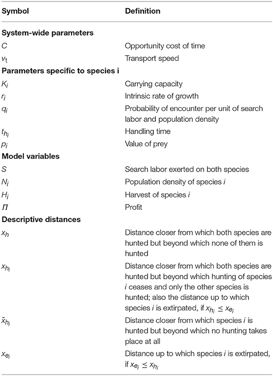
Table 1. Definitions of the symbols used in the model.

We will here develop further the spatial model of Sirén and Parvinen (2015) by including not only one but two prey species, in accordance with the non-spatial two-species model of Milner-Gulland and Mace (1998, pp. 72–77). In this model, the two species interact by being harvested together, but they have no other ecological interactions. This leads to the following form for the equations of growth of each of the species and for the profit made by the harvesters:

The two species may be of greatly different size and mass, and the use of the same transport speed, v_t, for both species therefore requires that this parameter is defined as the speed of transport per unit of mass, rather than per number of hunted prey. Accordingly, also the harvest variable, H_i, must be defined not as number of hunted prey animals, but as the mass of harvested matter and the handling time, t_hi, scaled to the mass of harvested matter.

In the standard model, we would have always H_i = q_iSN_i, but when the model includes the handling cost and the cost of transport, it may be that although it is profitable to have a positive search labor S, it is only beneficial to harvest one species. This occurs when the price of one species does not cover the handling and transport costs, so that

At a biological (ecological) equilibrium, the populations of the two species remain constant, i.e., we have $\frac{d{N}_1}{dt}=\frac{d{N}_2}{dt}=0$. We assume an open access scenario, where many individuals harvest resources from a common resource pool in an uncoordinated and self-interested manner. Under such conditions, hunters will not hunt species that are too costly to handle or transport. Therefore

The first row of Equation (9) tells us that the species N_i occurs at natural densities, i.e., carrying capacity, at the distance x if either its value p_i is so low that it does not make up for the inevitable costs of handling and transport or, alternatively, hunters are simply absent (S = 0). The second and third rows correspond to two situations in which the value p_i is high enough so that hunting species N_i is profitable at least if search costs are neglected. The third row tells us that a species is extirpated at the distance x, if its value is larger than the costs of handling and transport, and the search labor exerted by hunters exceeds a threshold determined by the species' intrinsic growth rate and the species' catchability coefficient. The middle row, finally, tells us that, in all other cases, the species in question will occur at a density larger than zero but smaller than the carrying capacity and which will be determined by the local search effort exerted by hunters (S) and the species-specific parameters carrying capacity (K_i), catchability coefficient (q_i), and intrinsic growth rate (r_i).

Extinction of both species at the same location is not possible in this model. According to Equation (9), species 1 will be extinct (N₁ = 0) if the marginal benefits are not negative, $p_i\ge c{t}_{{\text{h}}_{\text{i}}}+c\frac{x}{v_t}$ and search labor is large enough, $\overline{S}\ge \frac{r_1}{q_1}$, where $\overline{S}$ is the search time resulting from hunting of species 2 alone. The expression for profit when species 1 is locally extirpated and only species 2 is hunted is obtained from Equation (7) by substituting H₁ = 0 and H₂ = q₂SN₂, and we get

Next, we consider extinction of species 1 in a bioeconomic equilibrium, so that in addition to Equation (9), ∏ = 0 holds. Solving ∏ = 0 with (Equation 10) for N₂, we get the zero-profit population size of species 2 when species 1 is locally extirpated:

The zero-profit population size N₂ obtained from Equation (11) should agree with the equilibrium population size given by the second row of Equation (9), which results in the following condition for S:

Solving (Equation 12) with S > 0 is possible, if $\frac{c}{q_2\left(p_2-c{t}_{h_2}-\frac{cx}{v_t}\right)}<K_2$. Solving S from Equation (12), we obtain that the amount of local search labor in a bioeconomic equilibrium, when species 1 is not present, is

For the species 1 to be extirpated, we have the condition $\overline{S}\ge \frac{r_1}{q_1}$ (Equation 9). Substituting (Equation 13), we obtain

Solving (Equation 14) with equality for x, we obtain what we call the extinction distance, x_e1, for species 1, meaning that species 1 is present only beyond this distance, having been extirpated by hunting at closer distances to the central place from which hunters start their hunting journeys:

The conditions for the prices come from the third row of Equation (9) and are needed to ensure that handling and transporting both species are profitable at the distance given by the expression x_e1. Together with the condition $\frac{r_1}{q_1}<\frac{r_2}{q_2}$, this means that the third row of Equation (9) may hold for species 1 and the second row for species 2. If either of the price conditions does not hold, the extinction distance is given by the minimum of x_h1 and x_h2.

Analogously, the extinction distance for species 2 is

Note that only the species with lower ratio $\frac{r_i}{q_i}$ may become extirpated.

Next, we consider the distance beyond which either of the species is not harvested, so that the first row of Equation (9) holds. As no harvesting of species i occurs if the price does not cover handling and transport costs, i.e., if $p_i<c{t}_{h_i}+c\frac{x}{v_t}$ (Equation 9), we get from solving $p_i=c{t}_{h_i}+c\frac{x}{v_t}$ for x that species i will not be harvested further than

From now on, we assume that x_hi > 0. The second row of Equation (17) corresponds to a situation in which the price does not even cover handling costs alone. The actual no-harvest distance may also be even shorter than the expression x_hi given by the first row of Equation (17), because this does not take search costs into account. This is therefore a precise no-harvest distance only in the case that the other species is significantly more profitable to hunt, such that the search costs are covered by hunting for that species.

When the species are similar—but not necessarily equal—in their price and handling time, they have the same no-harvest distance. We can solve this no-harvest distance by substituting H_i = q_iSK_i in Equation (7) and solving for x from ∏ = 0, i.e.,

resulting in the common no-harvest distance

provided that harvesting both species at that distance would be profitable without search costs: $p_i\ge c{t}_{h_i}+c\frac{x_{\text{h}}}{v_{\text{t}}}$, or equivalently x_hi ≥ x_h, for both i.

However, when the species are not similar enough in their price and handling time, it is possible that for one species, $p_i<c{t}_{h_i}+c\frac{x_{\text{h}}}{v_{\text{t}}}$, i.e., x_hi < x_h, so that at the distance x_h given by Equation (19), it would not be profitable to hunt species i even without search costs. In such a situation, hunting the other species is very profitable and the hunters earn better simply by neglecting species i. As the search costs are covered by hunting the other species, the species i will then have no-harvest distance given by x_hi. For the other species (= j), we have at the no-harvest distance

which is obtained by substituting H_i = 0 and H_j = q_jSK_j in Equation (7) and setting ∏ = 0. The no-harvest distance for species j is then obtained by solving for x from Equation (20), resulting in

Note that the formulas satisfy $x_{e_1}<{\tilde{x}}_{h_2}$, when $\frac{r_1}{q_1}<\frac{r_2}{q_2}$, because species 2 can cause the extinction of species 1 only if species 2 is harvested at that distance. Furthermore, ${\tilde{x}}_{{\mathrm{\text{h}}}_2}<x_{h_2}$, which means that potential no-harvest distance ${\tilde{x}}_{h_2}$ derived assuming that search costs are covered by hunting species 2 only is strictly smaller than the upper bound x_h2 of the extinction distance derived from the marginal benefits, neglecting search costs.

Furthermore, the common no-harvest distance x_h from Equation (19) can be written as

so that x_h is a biased average of x_h1 and ${\tilde{x}}_{h_2}$, and analogously, a biased average of ${\tilde{x}}_{h_1}$ and x_h2. Since an average of two values is always in between the two values the average is taken from, we have the relations

In principle, we could have four different cases in which inequalities in Equation (23) hold. However, inequalities $x_{h_1}<{\tilde{x}}_{h_2}$ and $x_{h_2}<{\tilde{x}}_{h_1}$ cannot hold at the same time, because then from Equation (23), we would have x_h1 < x_h and $x_h<{\tilde{x}}_{h_1}$, so that $x_{{\text{h}}_1}<{\tilde{x}}_{h_1}$, which leads to contradiction. Overall, we have, thus, three different cases of no-harvest distances, and in different parts of the parameter space, we have different formulas determining the no-harvest distances summarized in Table 2.

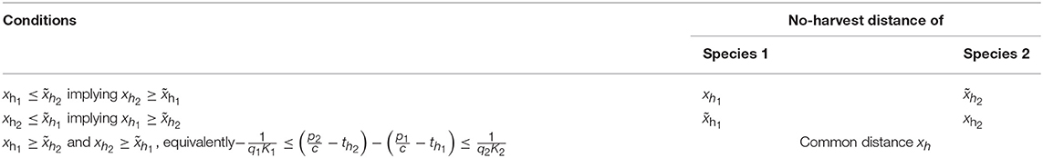
Table 2. The different cases of no-harvest distances.

Model Results

Figure 1 shows the two basic patterns that might occur depending on the r/q quotient of the two species, when all other parameters are equal or almost equal (here there is a minor difference of K between the two species, just in order to improve the visual presentation, avoiding that the curves for the two respective species overlap each other). When the r/q ratio is equal or similar between the two species, they coexist over the entire range of distances, depending on the parameter values (Figure 1A), but when their r/q ratios differ, the species with lower r/q may get extinct up to a certain distance, which we call the extinction distance. When cost-related parameters of the two species are similar (in Figure 1 they are the same), the no-harvest distance, i.e., the distance beyond which a species is not hunted at all, however, is the same for both species, regardless of the difference in r/q quotient.

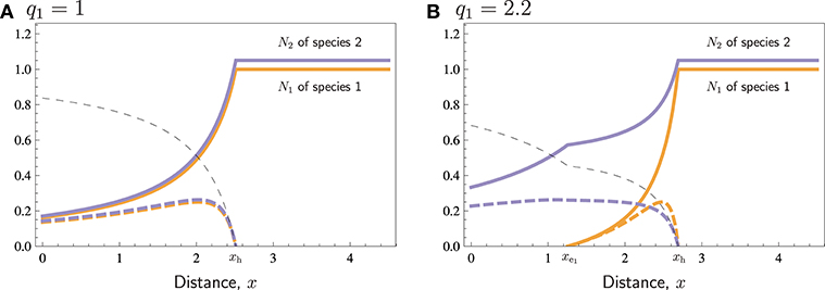
Figure 1. Typical cases for similar species. Population densities N₁ and N₂ (thick curves), harvest H₁ and H₂ (thick dashed curves), and search labor S (thin dashed curve) in a bioeconomic equilibrium with respect to distance x. (A) No extinction. (B) Species 1 is overharvested to extinction near the village, at distances 0 ≤ x ≤ ${\tilde{x}}_{e_1}$. In both cases harvesting becomes non-beneficial at long distances, for x ≥ x_h. Parameters: K₁ = 1, K₂ = 1.05, r₁ = r₂ = 1, q₂ = 1, p₁ = p₂ = 4, c = 1, t_h1 = t_h2 = 1, v_t = 1.

Figure 2 shows with some more detail how different values of r and q affect extinction distances and no-harvest distances. According to Equation (14), when the parameters r and q of the two species are close to being equal, one species cannot cause the extinction of the other species, as in those regions of Figure 2A, where r₁ ≈ r₂ = 1, and in Figures 2B,C, in those regions where q₁ ≈ q₂ = 1. If there is a considerable difference in the r/q quotient between the two species, however, the species with the lower ratio $\frac{r_i}{q_i}$ of growth rate and catchability may go extinct at short distances. For r₁, this is illustrated in Figure 2A: species 1 goes extinct when r₁ is low, and species 2 goes extinct when r₁ is large. The same phenomenon occurs in Figures 2B,C, when q₁ is large, as it is species 1, which has lower ratio $\frac{r_i}{q_i}$, that goes extinct. For low q₁, however, comparing the ratios $\frac{r_i}{q_i}$ only is not sufficient. Especially, when q₁ = 0, species 1 is not harvested at all, so that the model is essentially a one-species model, in which harvesting cannot cause extinction. Consequently, if extinction of species 2 occurs for some q₁ < q₂, it only occurs for intermediate values of q₁ (Figure 2C), and the extinction distance has a humped shape reaching a maximum at $q_1=\frac{q_2{r}_1}{2r_2}$ (at $q_1=\frac{1}{2}$ in Figure 2C). It is also possible that extinction of species 2 does not occur for any q₁ < q₂, even though species 2 then has lower ratio $\frac{r_i}{q_i}$ (Figure 2B). Such a situation occurs, when $\frac{p_1}{c}-t_{{\text{h}}_1}-4\frac{r_2}{q_2{r}_1{K}_1}<0$. In Figures 2B,C, we have $\frac{p_1}{c}-t_{h_1}-4\frac{r_2}{q_2{r}_1{K}_1}=3-\frac{4}{K_1}$, so that in Figure 2B we have $3-\frac{4}{K_1}=-1<0$, and in Figure 2C $3-\frac{4}{K_1}=1>0$. Again, since the cost-related parameters of the two species are similar (the same in Figure 2), the no-harvest distance still is identical (x_h given by Equation 19) for both species in all these cases, and x_h increases with q₁, but is unaffected by r₁.

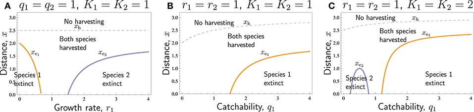
Figure 2. The common no- harvest distance x_h (thin dashed curve) and extinction distances x_e1 and x_e2 (thick solid curves) with respect to (A) r₁ and (B,C) q₁ for otherwise similar species. The curves separate areas with different type of presence of species (text labels). Other parameters: r₂ = 1, q₂ = 1, p₁ = p₂ = 4, c = 1, t_h1 = t_h2 = 1, v_t = 1.

In Figure 2, all species-specific parameters were the same for the two species, except for r_i or q_i. If $\frac{r_1}{q_1}=\frac{r_2}{q_2}$, the condition (Equation 14) for overharvested extinction is not satisfied. Therefore, it is meaningful to investigate the effect of other parameters on extinction distances only if $\frac{r_1}{q_1}\ne \frac{r_2}{q_2}$. This is illustrated in Figure 3, in which we have chosen such parameters that $\frac{r_1}{q_1}<\frac{r_2}{q_2}$, such that species 1 is the more vulnerable species and the only one that may be driven to extinction.

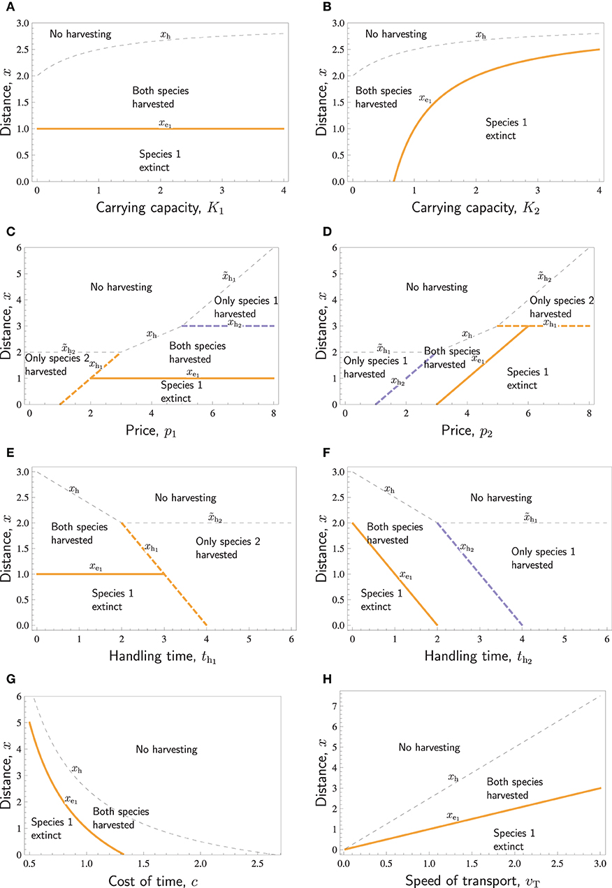
Figure 3. Distances with respect to various parameters: The no-harvest distances x_h, ${\tilde{x}}_{{\text{h}}_1}$, and ${\tilde{x}}_{{\text{h}}_2}$ (thin dashed curves) separating the areas of no harvesting and some harvesting, the no-harvest distances x_h1 and x_h2 (thick dashed curves) separating the areas of only one species harvested and both species harvested (potentially leading to the extinction of one of them), and the extinction distance x_e1, separating the areas where both species are successfully harvested, and where harvesting of both species results in the extinction of species 1 (thick solid curves). Species differ in r₁ = 0.5 < r₂ = 1. Except for the parameter displayed in the horizontal axis of each panel, the parameters are as follows: K₁ = K₂ = 1, q_l = q₂ = 1, p₁ = P₂ = 4, c = 1, t_h1 = t_h2 = 1, v_t = 1.

Increasing either one of the carrying capacities increases the overall abundance of prey and thus makes it profitable to hunt further away from the village, such that the no-harvest distance increases (Figures 3A,B). The carrying capacity K₁ of species 1 does not affect the extinction distance of the species 1 itself, $\frac{d}{d{K}_1}{x}_{e_1}=0$ (Figure 3A). In contrast, increasing the carrying capacity K₂ of species 2 leads to increased search labor and, therefore, increased extinction distance of species 1, $\frac{\text{d}}{\mathrm{\text{d}}{K}_2}{x}_{e_1}>0$ (Figure 3B).

Figures 3C,D illustrates the effects of prices p₁ and p₂. Increasing either one of the prices will make harvesting further away economically more profitable, and the no-harvesting distances x_h, x_hi, and ${\tilde{x}}_{h_i}$either increase linearly with p_i or are constants (actually, all curves separating different areas in Figures 3C,D are straight lines). If the prices of the two respective species differ very much, the species with the lower price is not harvested at all. If the price of one species is large, then far from the village only that species is harvested. Closer to the village, both species are harvested unless species 1 is extinct. Increasing either one of the prices may cause the extinction of species 1. Increasing p₁ does this by increasing the profitability of hunting species 1, and increasing p₂ does this by increasing the search effort. An interesting feature in Figures 3C,D is that the region “Species 1 extinct” borders to the region “Only species 2 harvested.” This implies that in a certain range of prices (see the line x_h1 in the intervals 1 < p₁ < 2 in Figure 3C and p₂ > 6 in Figure 3D), species 1 is hunted to extinction up to a certain distance, beyond which harvest of that species abruptly ceases, and it is present at its carrying capacity.

Handling times have similar effects as prices, but the patterns are reversed (Figures 3E,F). If handling time is too long for a species, it will not be harvested. For intermediate handling times, both species are harvested. Decreasing either one of the handling times may cause the extinction of species 1. Decreasing t_h1 does this by increasing the profitability of hunting species 1, and decreasing t_h2 does this by increasing the search effort. Also, in these panels, the curves separating different areas are straight lines.

The last two panels of Figure 3 show the effects of system-wide parameters. Figure 3G shows that if the cost of time c is large, then no harvesting takes place. This happens at least when t_h1c > p₁ and t_h2c > p₂. For low cost, the species with lower ratio $\frac{r_i}{q_i}$ goes extinct. For intermediate c, both species may be harvested. Figure 3H, on the other hand, shows that both the extinction distance and no-harvest distance increase linearly with respect to the speed of transport, v_t. Whereas the transport speed, v_t, and the cost of time, c, have opposite effects, there is one additional important difference. Doubling the transport speed always leads to a doubling of the extinction distance as well as the no-harvest distance, and only at v_t = 0 (an unrealistic scenario with completely sessile hunters), there is no local extinction at any distance. In contrast, doubling the cost of time reduces the extinction distance, as well as the no-harvest distance, with much more than half, and at a certain level of c, the extinction distance hits zero, as does also, at an even higher c, the no-harvest distance.

Discussion

This piece of research provides mathematical explanations to the commonly observed phenomenon that different species that are hunted together tend to not only differ in abundance as such but also show qualitatively different spatial patterns of abundance. Model results show a wide variety of possible scenarios when two species are hunted together, depending on how the parameter values of the two species differ from each other. Some of these results have potentially important implications for understanding the causes behind hunting-induced extirpations and practical wildlife management. For example, model results indicate that the extinction distance as well as the no-harvest distance are piecewise smooth—in relation to price or handling time (Figures 3C–F) even linear—functions that abruptly change slope at certain parameter values. For another part, model results suggest that even modest increases of the opportunity cost of time can have very positive effects on hunted wildlife populations, as the extinction distance is reduced with a factor larger than the factor of increase of the cost (Figure 3G).

All models are simplifications of reality, and it is therefore important to discuss the implications of the assumptions implicit in the model. For the single-species version of the model, Sirén and Parvinen (2015) discussed, for example, the implications (1) that it was deterministic, whereas real-life hunting involves a great deal of stochasticity; (2) that it had just one spatial dimension; (3) that it assumed that hunters have one single start- and endpoint for hunting trips; (4) that it considered travel and search as two separate activities; and (5) that it involved no animal movements. Some of these assumptions have still additional implications for the two-species model and the discussion of local extirpations.

Regarding the assumption of no dispersal or movements of animals, Novaro et al. (2000) argued that dispersal could have a key role in rebuilding animal populations depleted by hunting in tropical forests, and this was also supported by Sirén et al. (2004), who showed that, despite the dispersal rates for most major game species being relatively low, they were large enough to ensure that practically no species were permanently absent anywhere in the study area. Even the most severely depleted species, such as spider monkeys (Ateles belzebuth), were at rare occasions spotted (and killed) even very near the village. Thus, extinction according to the model should not be interpreted as a constant and complete absence of a species in real life, but rather as absence of breeding and reliance on a continuous influx due to source–sink dynamics in order to maintain a very low abundance or even just intermittent presence

Similarly, the model assumes a fixed handling time for each respective species. In reality, this can vary considerably. Any species might suddenly, by chance, appear within shooting range in front of a hunter, such that the handling time becomes minimal. At other times, the hunter might just hear the animal at a distance, requiring the hunter to carefully pursue it, without making noise that scares it away. Some species, such as large rodents, armadillos, and the white-collared peccary (Tayassu pecari) commonly take escape in burrows when stalked by dogs, and it can then be a quite lengthy procedure to kill them and recover the carcass from inside the burrow. Rather than a fixed handling time for each species, in real life, there is just a different probability for different handling times for each species. In addition, as also the cost of ammunition is included in this parameter, another cause of variability is that sometimes hunters miss the target, thus having to shoot more than once or, in worst case, wasting ammunition but failing to recover the prey. Again, therefore, the model predictions in Figure 3 should not be taken too literally. That the model predicts that for some combinations of parameter values one of the species is not hunted does not mean that in real life it will not be hunted at all, but rather that it will be hunted in relatively small numbers.

Although the inclusion of two species is an important improvement in comparison with the single-species model, it is still a major simplification, as empirical studies indicate that tropical forest hunters tend to hunt a large number of different species, ranging from around 20 (Ohl-Schacherer et al., 2007) to around 40 (Franzen, 2006), or 60 (Sirén, 2012; Constantino, 2016). It should also be noted that in this model the two species do not interact with each other in any other way than that they are harvested together.

Some of these limitations of the model could, in principle, be resolved relatively easily. For example, including ecological interactions between the two species, such as competition for resources, would also be relatively straightforward (cf. Milner-Gulland and Mace, 1998, pp. 71–77). It would also be possible to include multiple species in the model or to introduce stochasticity. The more complex a model becomes, however, it also becomes less perspicuous, and the whole point of analytical models is to highlight some certain aspects of reality, which requires disregarding others. This two-species model can help us gain important insights into the spatial patterns of harvest and abundance and the mechanisms leading to sequential extirpations, in space and time, of certain species in harvested multispecies systems (cf. Rowcliffe et al., 2003). There is ample empirical evidence showing that animal species with certain traits (particularly, large bodied, large group living, arboreal, and diurnal) are more susceptible to extirpation due to hunting than others (e.g., Ripple et al., 2016; Abrahams et al., 2017). However, it is not well-understood how such characteristics of different species interact with each other and with socioeconomic parameters in order to produce different outcomes in terms of local extirpations of some of the species. We believe that the model presented here can help to gain a better theoretical understanding of the mechanisms leading to sequential extirpation of different game species and of the spatial distribution of the so-called “extinction envelopes” (cf. Shaffer et al., 2018) of different species.

Theoretical models should ideally always be validated by comparison with empirical data, but this involves, in this case, considerable challenges and is beyond the scope of this piece of research. In order to fully validate this model, one would need a large set of empirical data including spatially explicit data on wildlife harvest and abundance as well as trustworthy estimates of key biological and economic parameters for each hunted wildlife species. In addition, such a dataset would need to cover a wide range of variability in the opportunity cost of time, as well as within-species and between-species variabilities in price and handling time (the latter mediated by technology). Currently, however, there is no dataset available that is even close to fulfilling these criteria. It remains an open question whether it would be feasible to construct such a dataset even by pooling together data from many different case studies, conducted by different researchers in different parts of the world.

An alternative approach to validating the model, however, could be to look for cases in the real world where a hunted species qualitatively behaves like the model predicts. Such a case could be, for example, that a species with lower market price or use value than most other prey species is hunted to extirpation up to a certain distance, but is not hunted at all beyond this distance, as predicted by Figures 3C,D, where the line x_h1 separates the area “Species 1 extinct” from “Only species 2 harvested.” Another such case could be that a relatively modest increase of the price of some species that previously have not been hunted leads to extirpation of the species over a significant distance, but that this extinction distance afterward remains relatively constant despite further increases of price, as in Figure 3C, where the slope of line x_e1is horizontal, or, analogously, the same phenomenon for reduced handling time, due to some technological improvement, as in Figure 3E.

Whereas we here have analyzed only the case of open access hunting, a next step will be to analyze also the social optimum case, as Sirén and Parvinen (2015) did for the one-species version of this model, and also to analyze the economic and ecological effects of different sorts of hunting regulations and enforcement strategies (cf. Albers, 2010). Because of the huge challenges involved in collecting empirical data on the parameters and variables included in models of hunting in tropical forests (cf. Carrillo et al., 2000; Van Vliet and Nasi, 2008), practical wildlife management will have to rely more on trial and error than on prescriptions based on quantitative modeling (cf. Johannes, 1998). Analytical models like this one could be a useful support, however, when trying to figure out which management measures might be worthwhile to try out in the real world.

Author Contributions

AS formulated the basic characteristics of the model, defined the questions to be answered, and wrote the Background and Discussion sections. KP did most of the mathematical analyses, designed the figures, and wrote most of the sections Model Assumptions and Model Results.

Funding

We were granted a waiver from Frontiers for 50% of the article processing fee, and CIFOR provides the remaining 50%.

Conflict of Interest Statement

The authors declare that the research was conducted in the absence of any commercial or financial relationships that could be construed as a potential conflict of interest.

References

Abrahams, M. I., Peres, C. A., and Costa, H. C. (2017). Measuring local depletion of terrestrial game vertebrates by central-place hunters in rural Amazonia. PLoS ONE 12:e0186653. doi: 10.1371/journal.pone.0186653
Albers, H. J. (2010). Spatial modeling of extraction and enforcement in developing country protected areas. Resour. Energy Econ. 32, 165–179. doi: 10.1016/j.reseneeco.2009.11.011
Alvard, M. S. (1993). Testing the “ecologically noble savage” hypothesis: interspecific prey choice by Piro hunters of Amazonian Peru. Hum. Ecol. 21, 355–387. doi: 10.1007/BF00891140
Apaza, L., Wilkie, D., Byron, E., Huanca, T., Leonard, W., Pérez, E., et al. (2002). Meat prices influence the consumption of wildlife by the Tsimane' Amerindians of Bolivia. Oryx 36, 382–388. doi: 10.1017/S003060530200073X
Carrillo, E., Wong, G., and Cuarón, A. D. (2000). Monitoring mammal populations in Costa Rican protected areas under different hunting restrictions. Conserv. Biol. 14, 1580–1591. doi: 10.1111/j.1523-1739.2000.99103.x
Cawthorn, D. M., and Hoffman, L. C. (2015). The bushmeat and food security nexus: a global account of the contributions, conundrums and ethical collisions. Food Res. Int. 76, 906–925. doi: 10.1016/j.foodres.2015.03.025
Charnov, E. L. (1976). Optimal foraging: attack strategy of a mantid. Am. Nat. 110, 141–151. doi: 10.1086/283054
Constantino, P. A. L. (2016). Deforestation and hunting effects on wildlife across Amazonian indigenous lands. Ecol. Soc. 21:3. doi: 10.5751/ES-08323-210203
Damania, R., Milner-Gulland, E. J., and Crookes, D. (2005). A bioeconomic analysis of bushmeat hunting. Proc. R. Soc. B 272, 259–266. doi: 10.1098/rspb.2004.2945
Demmer, J., Godoy, R., Wilkie, D., Overman, H., Taimur, M., Fernando, K., et al. (2002). Do levels of income explain differences in game abundance? An empirical test in two Honduran villages. Biodivers. Conserv. 11, 1845–1868. doi: 10.1023/A:1020305903156
Foerster, S., Wilkie, D. S., Morelli, G. A., Demmer, J., Starkey, M., Telfer, P., et al. (2012). Correlates of bushmeat hunting among remote rural households in Gabon, Central Africa. Conserv. Biol. 26, 335–344. doi: 10.1111/j.1523-1739.2011.01802.x
Franzen, M. (2006). Evaluating the sustainability of hunting: a comparison of harvest profiles across three Huaorani communities. Environ. Conserv. 33, 36–45. doi: 10.1017/S0376892906002712
Godoy, R., Undurraga, E. A., Wilkie, D., Reyes-García, V., Huanca, T., Leonard, W. R., et al. (2010). The effect of wealth and real income on wildlife consumption among native Amazonians in Bolivia: estimates of annual trends with longitudinal household data (2002–2006). Anim. Conserv. 13, 265–274. doi: 10.1111/j.1469-1795.2009.00330.x
Hames, R. B., and Vickers, W. T. (1982). Optimal diet breadth theory as a model to explain variability in Amazonian hunting. Am. Ethnol. 9, 358–378. doi: 10.1525/ae.1982.9.2.02a00090
Johannes, R. E. (1998). The case for data-less marine resource management: examples from tropical nearshore finfisheries. Trends Ecol. Evol. 13, 243–246. doi: 10.1016/S0169-5347(98)01384-6
Keeling, M. J., Milner-Gulland, E. J., and Clayton, L. M. (1999). Spatial dynamics of two harvested wild pig populations. Nat. Resour. Model. 12, 147–169. doi: 10.1111/j.1939-7445.1999.tb00007.x
Levi, T., Lu, F., Yu, D. W., and Mangel, M. (2011). The behaviour and diet breadth of central-place foragers: an application to human hunters and Neotropical game management. Evol. Ecol. Res. 13, 171–185.
Ling, S., and Milner-Gulland, E. J. (2006). Assessment of the sustainability of bushmeat hunting based on dynamic bioeconomic models. Conserv. Biol. 20, 1294–1299. doi: 10.1111/j.1523-1739.2006.00414.x
Ling, S., and Milner-Gulland, E. J. (2008). When does spatial structure matter in models of wildlife harvesting? J. Appl. Ecol. 45, 63–71. doi: 10.1111/j.1365-2664.2007.01391.x
Milner-Gulland, E. J., Bunnefeld, N., and Proaktor, G. (2009). “The science of sustainable hunting,” in Recreational Hunting, Conservation and Rural Livelihoods (Oxford: Wiley-Blackwell), 75–93.
Milner-Gulland, E. J., and Mace, R. (1998). Conservation of Biological Resources. Oxford: Blackwell Science Ltd.
Novaro, A. J., Redford, K. H., and Bodmer, R. E. (2000). Effect of hunting in source–sink systems in the neotropics. Conserv. Biol. 14, 713–721. doi: 10.1046/j.1523-1739.2000.98452.x
Ohl-Schacherer, J., Shepard, G. H., Kaplan, H., Peres, C. A., Levi, T., and Yu, D. W. (2007). The sustainability of subsistence hunting by Matsigenka native communities in Manu National Park, Peru. Conserv. Biol. 21, 1174–1185. doi: 10.1111/j.1523-1739.2007.00759.x
Overman, H., and Demmer, J. (1999). The Effects of Wealth on The Use of Forest Resources: The Case of the Tawahka Amerindians, Honduras. Wageningen: Tropenbos International.
Peres, C. A., and Lake, I. R. (2003). Extent of nontimber resource extraction in tropical forests: accessibility to game vertebrates by hunters in the Amazon basin. Conserv. Biol. 17, 521–535. doi: 10.1046/j.1523-1739.2003.01413.x
Ripple, W. J., Abernethy, K., Betts, M. G., Chapron, G., Dirzo, R., Galetti, M., et al. (2016). Bushmeat hunting and extinction risk to the world's mammals. R. Soc. Open Sci. 3:160498. doi: 10.1098/rsos.160498
Robinson, B. E. (2016). Conservation vs. livelihoods: spatial management of non-timber forest product harvests in a two-dimensional model. Ecol. Appl. 26, 1170–1185. doi: 10.1890/14-2483
Rowcliffe, J. M., Cowlishaw, G., and Long, J. (2003). A model of human hunting impacts in multi-prey communities. J. Appl. Ecol. 40, 872–889. doi: 10.1046/j.1365-2664.2003.00841.x
Shaffer, C. A., Yukuma, C., Marawanaru, E., and Suse, P. (2018). Assessing the sustainability of Waiwai subsistence hunting in Guyana by comparison of static indices and spatially explicit, biodemographic models. Anim. Conserv. 21, 148–158. doi: 10.1111/acv.12366
Shively, G. E. (1997). Poverty, technology, and wildlife hunting in Palawan. Environ. Conserv. 24, 57–63. doi: 10.1017/S0376892997000106
Sirén, A. (2012). Festival hunting by the Kichwa people in the Ecuadorian Amazon. J. Ethnobiol. 32, 30–50. doi: 10.2993/0278-0771-32.1.30
Sirén, A., Hambäck, P., and Machoa, J. (2004). Including spatial heterogeneity and animal dispersal when evaluating hunting: a model analysis and an empirical assessment in an Amazonian community. Conserv. Biol. 18, 1315–1329. doi: 10.1111/j.1523-1739.2004.00024.x
Sirén, A., and Parvinen, K. (2015). A spatial bioeconomic model of the harvest of wild plants and animals. Ecol. Econ. 116, 201–210. doi: 10.1016/j.ecolecon.2015.04.015
Sirén, A. H., Cardenas, J. C., Hambäck, P., and Parvinen, K. (2013). Distance friction and the cost of hunting in tropical forest. Land Econ. 89, 558–574. doi: 10.3368/le.89.3.558
Sirén, A. H., and Wilkie, D. S. (2016). The effects of ammunition price on subsistence hunting in an Amazonian village. Oryx 50, 47–55. doi: 10.1017/S003060531400026X
Smith, D. A. (2003). Participatory mapping of community lands and hunting yields among the Buglé of western Panama. Hum. Organ. 332–343. doi: 10.17730/humo.62.4.cye51kbmmjkc168k
Stephens, D. W., and Krebs, J. R. (1986). Foraging Theory, 1st Edn. Princeton, NJ: Princeton University Press.
Stirnemann, R. L., Stirnemann, I. A., Abbot, D., Biggs, D., and Heinsohn, R. (2018). Interactive impacts of by-catch take and elite consumption of illegal wildlife. Biodivers. Conserv. 27, 931–946. doi: 10.1007/s10531-017-1473-y
Van Vliet, N., and Nasi, R. (2008). Why do models fail to assess properly the sustainability of duiker (Cephalophus spp.) hunting in Central Africa? Oryx 42, 392–399. doi: 10.1017/S0030605308000288
Vasco, C., and Sirén, A. (2016). Correlates of wildlife hunting in indigenous communities in the Pastaza province, Ecuadorian Amazonia. Anim. Conserv. 19, 422–429. doi: 10.1111/acv.12259
Wilkie, D. S., and Godoy, R. A. (2001). Income and price elasticities of bushmeat demand in lowland Amerindian societies. Conserv. Biol. 15, 761–769. doi: 10.1046/j.1523-1739.2001.015003761.x
Keywords: extinction, transport, handling, central place foraging, bushmeat, wildlife, bioeconomic equilibrium, tropics
Citation: Sirén AH and Parvinen K (2019) Bioeconomic Modeling of Hunting in a Spatially Structured System With Two Prey Species. Front. Ecol. Evol. 7:268. doi: 10.3389/fevo.2019.00268
Received: 01 February 2019; Accepted: 25 June 2019;
Published: 17 July 2019.
Edited by:
Robert Nasi, Center for International Forestry Research, IndonesiaReviewed by:
Viorel Dan Popescu, Ohio University, United StatesKatharine Anne Abernethy, University of Stirling, United Kingdom
Copyright © 2019 Sirén and Parvinen. This is an open-access article distributed under the terms of the Creative Commons Attribution License (CC BY). The use, distribution or reproduction in other forums is permitted, provided the original author(s) and the copyright owner(s) are credited and that the original publication in this journal is cited, in accordance with accepted academic practice. No use, distribution or reproduction is permitted which does not comply with these terms.
*Correspondence: Anders Henrik Sirén, anders.siren@utu.fi