Maps From Mud—Using the Multiple Scenario Approach to Reconstruct Land Cover Dynamics From Pollen Records: A Case Study of Two Neolithic Landscapes
 M. Jane Bunting
 Michelle Farrell
 Alex Bayliss
 Peter Marshall4
 - 1Geography, School of Environmental Sciences, University of Hull, Hull, United Kingdom
- 2School of Energy, Construction and Environment, Coventry University, Coventry, United Kingdom
- 3Centre for Research in the Built and Natural Environment, Coventry University, Coventry, United Kingdom
- 4Historic England, London, United Kingdom
- 5Biological and Environmental Sciences, University of Stirling, Stirling, United Kingdom
- 6Department of Archaeology and Conservation, Cardiff University, University of Cardiff, Cardiff, United Kingdom
Pollen records contain a wide range of information about past land cover, but translation from the pollen diagram to other formats remains a challenge. In this paper, we present LandPolFlow, a software package enabling Multiple Scenario Approach (MSA) based land cover reconstruction from pollen records for specific landscapes. It has two components: a basic Geographic Information System which takes grids of landscape constraints (e.g., topography, geology) and generates possible “scenarios” of past land cover using a combination of probabilistic and deterministic placement rules to distribute defined plant communities within the landscape, and a pollen dispersal and deposition model which simulates pollen loading at specified points within each scenario and compares that statistically with actual pollen assemblages from the same location. Goodness of fit statistics from multiple pollen site locations are used to identify which scenarios are likely reconstructions of past land cover. We apply this approach to two case studies of Neolithisation in Britain, the first from the Somerset Levels and Moors and the second from Mainland, Orkney. Both landscapes contain significant evidence of Neolithic activity, but present contrasting contexts. In Somerset, wet-preserved Neolithic remains such as trackways are abundant, but little dry land settlement archaeology is known, and the pre-Neolithic landscape was extensively wooded. In Orkney, the Neolithic archaeology includes domestic and monumental stone-built structures forming a UNESCO World Heritage Site, and the pre-Neolithic landscape was largely treeless. Existing pollen records were collated from both landscapes and correlated within new chronological frameworks (presented elsewhere). This allowed pollen data to be grouped into 200 year periods, or “timeslices,” for reconstruction of land cover through time using the MSA. Reconstruction suggests that subtle but clear and persistent impacts of Neolithisation on land cover occurred in both landscapes, with no reduction in impact during periods when archaeological records suggest lower activity levels. By applying the methodology to specific landscapes, we critically evaluate the strengths and weaknesses and identify potential remedies, which we then expand into consideration of how simulation can be incorporated into palynological research practice. We argue that the MSA deserves a place within the palynologist's standard tool kit.
Introduction
Land cover is an important component of the earth system, through the habitats it provides for living things and through its interactions with the other major components, for example with the hydrosphere via modification of water flow and water quality, and with the atmosphere and climate system through albedo and evapotranspiration. Land cover develops in response to a range of environmental drivers, including climate zone, substrate, topography, and feedback interactions between biota and between biotic elements and the physical environment. Human activity is a major shaper of these feedback interactions, both directly (e.g., through tree felling, ploughing, or construction of novel habitats) and indirectly (e.g., through changing distributions and intensities of grazing animals, which in turn can reduce ground cover or transform forest into scrub or grassland). Land cover is variable in both space and time, and reconstructing past land cover is therefore an important contribution to understanding the longer-term dynamics of the earth system (for example for testing regional climate models or framing the context of archaeological records of human activity), as well as for ecological studies of ecosystem processes and dynamics and archaeological investigation of the controls on and environmental impacts of past human activity.
Pollen analysis offers a means of indirectly observing past vegetation, and therefore pollen records (sequences of pollen assemblages recovered from sedimentary archives such as mires or lake sediments) are an important source of information about past land cover. Translation of standard pollen diagrams—information-packed, but often an active barrier to engagement by non-specialists within and beyond academic communities because they are very difficult to read without extensive experience—into measures of land cover is an ongoing research challenge. Von Post (1918) and Edwards et al. (2017) described the task of the pollen analyst as being to “think horizontally, work vertically,” showing that from the earliest days of the discipline reconstruction of spatial variations in land cover at different points in the past was seen as the main goal of the activity. Pollen assemblages form through a complex combination of taphonomic processes reflecting both the biology and ecology of the plants producing the pollen and the shape, size, type, and setting of the sedimentary system where the assemblage forms and will be preserved, and therefore translation into land cover is not a trivial exercise, especially if the land cover measure is to be quantitative and spatially referenced rather than qualitative. Various methodologies have been explored, such as biomisation (e.g., Prentice et al., 1996), modern analog comparison methods (e.g., Overpeck et al., 1985), and the use of models of the relationship between pollen and vegetation or the process of pollen dispersal and deposition.
Algebraic models connecting pollen assemblages at a known location and the source vegetation in the wider landscape offer a means of reconstructing past land cover. The main approach currently in use is the Landscape Reconstruction Algorithm (LRA; Sugita, 2007a,b; Gaillard et al., 2008, 2010; Hellman S. et al., 2008; Trondman et al., 2015; PAGES, 2017). The LRA is not the only possible use of the algebraic models. Interpretation can also be informed by simulation studies or “thought experiments” (e.g., Bunting et al., 2004; Caseldine and Fyfe, 2006; Caseldine et al., 2007; Hellman et al., 2009a,b) using the HUMPOL suite (Middleton and Bunting, 2004; Bunting and Middleton, 2005). This approach was developed into the Multiple Scenario Approach (MSA; Bunting and Middleton, 2009); where the LRA takes an algebraic approach to reconstructing past land cover numerically, which can then be extrapolated into mapped forms (e.g., Pirzamanbein et al., 2014), the MSA uses computer simulations to produce many possible reconstructions, which are then tested using the model (see Figure 1 for a comparison of the two approaches). This paper presents two examples of the use of the MSA to address landscape-scale questions about land cover and land use during the Neolithic in the British Isles, and considers lessons learned for future development of this relatively new and under-explored method.
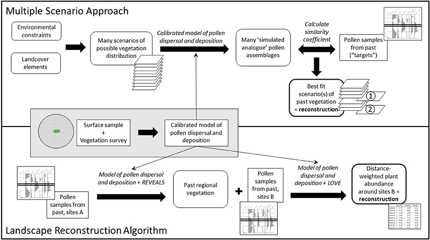
Figure 1. A schematic representation comparing two approaches to reconstruction of land cover from pollen assemblages, the Landscape Reconstruction Algorithm (LRA; Sugita, 2007a,b) and the Multiple Scenario Approach (MSA; Bunting and Middleton, 2009).
The nature of Neolithic agriculture in the British Isles remains poorly understood. Evidence for the prior presence of Mesolithic people is widespread, but their population levels were probably very low, and direct environmental impacts would have been localized. Impacts may have included modification of woodland structure (e.g., Bishop et al., 2015). The repeated use of fire, and possible knock-on effects on the location of wild native herbivores, particularly deer, are argued to have modified woodland edge habitats in the uplands (Innes et al., 2010, 2013; Ryan and Blackford, 2010) and at wetland margins (Mellars and Dark, 1998), at least in some locations and at some times. The early Holocene woodland cannot be considered pristine and unsettled, but existing evidence suggests that Mesolithic people caused only minor disturbance, with effects comparable to other components of the natural disturbance regime. Neolithisation introduced two new potential disturbance factors into the landscape, livestock management, and crop cultivation. The introduction of non-native herbivores, especially sheep and goats which are particularly effective at suppressing regeneration of deciduous woodland, and increased management of the numbers and locations of large animals in the landscape will have increased grazing and associated landscape effects such as creation of paths and trampling and erosion at watering points and gathering yards, which will both create small clearings and favour ruderal forb plant species over woodland understorey species.
Crop cultivation requires removal of pre-existing vegetation, especially in woodland, and management of soil fertility and weeds. Various models for achieving this have been suggested for Neolithic Europe, with strong evidence for long-term cultivation at specific locations (“gardens”) supported by manuring practices alongside cyclic use of the wider landscape through coppicing and movement of animal herds for the Central European lake dwellings area (Jacomet et al., 2016), although some argue that shifting “slash and burn” type cultivation would have been more effective in wooded areas (e.g., Schier, 2009; Rösch et al., 2017). In lowland areas of the UK, Neolithic practices were introduced into landscapes dominated by mixed deciduous woodland, and the pollen signal of Neolithisation is largely seen through an increase in non-arboreal pollen types reflecting the crops themselves, ruderal species associated with the newly available areas of disturbed ground, and the species which replaced the dominant canopy trees both in areas kept open by grazing and as part of the successional sequence once garden-patches were abandoned. Whilst the crops and settlements of these Neolithic populations will have occupied a very small fraction of a landscape at any one point in time, the effects of these cultural practices will have been more widely seen, both through the impacts of grazing livestock and through the persistence of an ecological signal of disturbance for decades and sometimes centuries following abandonment and movement of the farming population. However, not all parts of the UK were fully wooded at the start of the Neolithic, and some of the most exciting archaeological finds of recent years (e.g., Ness of Brodgar; Card et al., 2017) come from the far North, where woodland cover was probably never complete in the Holocene, and certainly by the mid-Holocene the landscape contained extensive areas of naturally treeless grassland. Here woodland did not have to be cleared to permit agricultural activity, and indeed may have been sufficiently limited that it required deliberate protection. The pollen signal of agricultural activity in such a landscape will probably lack the classic “decrease of tree pollen” signal of a “landnám” in a woodland area, but should still be seen through an increase in ruderal species and possibly crop plants.
In this paper, we use pollen records and the MSA to reconstruct the landscape level impact of Neolithisation on land cover in two contrasting British landscapes, the Somerset Levels and Moors and Mainland Orkney, both with a rich and well dated archaeological record of Neolithic activity which provides an indication of variations in the amount and intensity of activity over the period, for comparison with the reconstructed land cover record. The Somerset Levels are a complex of lowland wetlands within a densely wooded mid-Holocene landscape, with substantial tree removal only beginning to be recorded in the Iron Age. In Orkney, pollen records come from discrete basins scattered across Mainland, and the northerly, hyperoceanic setting of the islands meant that full forest cover probably never developed.
The aims of this paper are to:
(a) Use the pollen record for the Neolithic period (broadly defined) in two UK landscapes containing important Neolithic archaeology which have contrasting late-Mesolithic land cover, to reconstruct the extent and timing of land cover modification associated with Neolithisation and determine whether land cover changes occur in the same pattern as archaeologically-derived estimates of occupation levels.
(b) Consider the strengths and weaknesses of the MSA for land cover reconstruction.
(c) Demonstrate how pollen dispersal and deposition models and the MSA can be used to strengthen the relationship between pollen data and archaeological research questions, and be incorporated into the palynologist's standard workflow.
Materials and Methods
In this section we outline the MSA and introduce the case studies.
The Multiple Scenario Approach
The MSA is outlined in Bunting and Middleton (2009) and schematically presented in Figure 1. Reconstruction begins with a landscape of interest, from which one or more empirical pollen records covering the relevant time period are available.
First, the analyst identifies the main environmental constraints in that landscape which can be known for the relevant time period (e.g., topography, geology, paleogeography) and the palynological equivalent1 (hereafter p.e.) vegetation components which might have formed part of past land cover. These components can be a single p.e. (e.g., Quercus) which can represent one or many plant species, or a community comprising a defined mixture of p.e. taxa (e.g., every pixel assigned to grassland is modelled as containing 80% Poaceae, 10% Cyperaceae, and 10% Plantago lanceolata).
This information is used as input into a Geographic Information System (GIS) to create many possible maps of distribution of those land cover components, combining gridded environmental data with both environmental constraints (e.g., Quercus can only occur below 600 m asl) and random placement rules (for example a pixel in the area below 600 m has a 20% chance of being occupied by Quercus, a 10% chance of being occupied by Betula and a 70% chance of being occupied by grazed grassland) to assign each pixel in the grid to one of the vegetation components. For each of these possible maps, pollen assemblages are simulated at the location of the actual pollen records using a pollen dispersal and deposition model. These simulated pollen assemblages are then compared with the empirical pollen assemblages using similarity coefficients; scenarios producing the most similar pollen assemblages or similarity scores meeting some pre-determined criterion are considered to be possible reconstructions of the past land cover at the time when the pollen assemblage was formed.
One strength of this method is its ability to identify multiple different possible reconstructions, including arrangements of past land cover which are ecologically distinct (e.g., birch woodland and oak woodland or mixed birch-oak woodland, copses in open fields or wood-pasture; see Bunting and Farrell, 2017) but cannot be distinguished palynologically from the available pollen records. This both reduces analyst bias in favor of particular types of landscape and offers up clear alternative hypotheses for testing via either future pollen analysis or by seeking out other lines of evidence. Whereas LRA reconstructions are presented as percentage cover (for “regional” vegetation, e.g., an average for an area on the order of 50–100 km radius around the study sites) or distance weighted plant abundance (within the Relevant Source Area of Pollen for small sites, typically 500–2,000 m radius), which are then converted into spatial representations of land cover using GIS (see e.g., Pirzamanbein et al., 2014), MSA reconstructions are produced in a mapped form from which quantitative measures can be derived if required.
LandPolFlow Software Package
LandPolFlow is a specialist simplified GIS coded in Borland Delphi. The principal simplification made is the requirement that all gridded data are in raster format and for any given analysis run all grids have the same dimensions, resolution and geographic location, although there is some capacity to nest larger land cover grids or to otherwise incorporate a “background” pollen component sourced beyond the modelled landscape. LandPolFlow was written by Mr. R. Middleton, now retired from the University of Hull. The software is available on request from Dr. M. Jane Bunting (and via worktribe, the University of Hull repository).
Inputs: environmental data
Input grids define the physical environment on which land cover forms. The format used for all grid types is that used by the 16 bit (DOS) version of Idrisi and later by Openland (Eklöf et al., 2004) and HUMPOL (Bunting and Middleton, 2005). Three kinds of grids can be used, class grids (coded using numbers in the range 0–255) which can be linked to tables which assign numerical values to specific classes, Boolean grids and real data grids (containing quantitative information stored as IEEE single precision real values). Provision has been made within the package to derive slope and aspect grids from digital elevation models (DEMs), and to smooth the derived grids. In the examples presented here we use class grids for surficial geology and definition of known water bodies and coastline, and real grids for DEMs. A script file is then used to instruct the program to create one or more new grids with the same dimensions as the environmental grids, showing land cover classes. The available land cover classes are defined in a separate input file, the “PolSack” file (see section Simulated Pollen Assemblages below).
Scripts and scripting
All operations in LandPolFlow are performed under the control of a script file. The scripting language makes use of loops and system-defined variables (e.g., limiting altitudes, the probability of a particular land cover element being present) to allow many land cover grids to be made in a single run reflecting varying land cover placement “rules.” These placement “rules” can be prescriptive (e.g., Betula never occurs on limestone/above 600 m asl) or probabilistic (e.g., the likelihood of Betula occurring on steep slopes is 80%, on moderate slopes is 50% and on shallow slopes is 20%), and rule parameters can also be varied (e.g., maximum altitude can be 550, 600, 650 m asl etc., or the probability of occurrence on a moderate slope can vary between 10 and 50% in 4% steps). Land cover types can be placed into the grid as single pixels or as larger blocks within the landscape, allowing scenarios to explore the effects of different sizes of patches (e.g., the pollen signal of a farming landscape where human activity is centered around multiple scattered “farmsteads” vs. a single large “village”) as well as of different proportions of total cover. The number of grids defined by combinations of placement rules and taxa can be very large.
Simulated pollen assemblages
A second set of commands within the script simulate the pollen assemblage for a land cover grid at one or more specified locations, and calculate the similarity coefficient between the simulated assemblage and the actual target pollen assemblage. Two input files are required for these commands in addition to the environmental grids; the first defines the composition of the land cover classes, the properties of the pollen types produced by the p.e. taxa (e.g., Relative Pollen Productivity), and the specific locations for which pollen assemblages are to be simulated (the “PolSack” file), and the second is a lookup table containing taxon-specific distance weightings for each pollen type, based on the pollen dispersal and deposition model chosen. Using a lookup table increases the speed of calculation of simulated pollen loading, which is valuable when many possible land cover scenarios are being considered. Details of the calculations are presented in the Supplementary Material to this paper.
Handling output data
Software output is in two forms, as grids (which can be saved in IDRISI format, as jpegs or as bitmaps) and as a text file containing the simulated pollen assemblages, calculated fit statistics (a selection of similarity measures are available; in this study we used squared-chord distance) and other model parameters as defined by the user (e.g., the system variables used in the script loops to vary abundance or location of land cover classes). Within the script a saving threshold can be set to ensure that grids are only saved for scenarios with a good fit, reducing the memory demands of the program. Output files can then be processed in many ways. In this study, we used R scripts to help extract the output for best fit solutions for individual target locations and for the landscape as a whole from the text files (identified from the sum of fits for all target locations). Scripts are available from the authors on request.
Two approaches to identifying the “best” landscape reconstructions were used, a site-led approach and a whole-landscape approach. For the site-led approach, the best fit scenarios for each individual pollen core location were identified by the site fit score, and the overall landscape character determined as a mean of the model parameters for the scenarios providing those best fit scores with variation expressed as standard error around that mean. This site-led approach produces reconstructions of trends in land cover and changes between timeslices expressed in model parameters (e.g., probability that a pixel meeting specified criteria will be allocated “woodland”) rather than land cover parameters (e.g., hectares of woodland in the final grid). For the Somerset Levels and Moors dryland land cover reconstruction the average of parameters for the single best fit scenario for each pollen site was used. For the Orkney case study, where there were fewer pollen sites available, model parameter averages were taken from the best five fits for each site. This approach made more allowance for local variation in land cover both on and around each individual site than the whole-landscape approach, useful in this project where the number of repeat runs was limited (a high number of repeats of each scenario is ideally required since random placement of vegetation can lead to highly varied site pollen signals in sensitive locations).
For the whole landscape approach, the best-fit scenario was that which produced the lowest overall fit score based on the sum of scores for all sites, that is, it is effectively the reconstruction which offers the best compromise across the target pollen records. To extract land cover data in this approach, the best fit grid was saved and the coverage of each community within the grid determined using mosaic5 (updated from Middleton and Bunting, 2004) then converted into hectares.
Single grids for each timeslice were also selected to create a visual sequence of landscape development. These grids were chosen from the selection of grids saved by the software, i.e., those with fit scores below a pre-determined threshold. In most cases the grid with the lowest overall fit score was chosen, but in some cases a different grid was selected on grounds of being more “plausible” (sensu Caseldine et al., 2008)—that is, that it fitted logically into the sequence in such a way that known ecological processes could be evoked to explain the transition from and to the landscape scenarios on either side. There is considerable scope for improvement in determining the best and most efficient methods of extracting and presenting land cover data from MSA reconstruction output, but the methods chosen here are replicable and produce consistent and reasonable results.
Case Study Landscapes
The Somerset Levels and Moors (Figure 2) were chosen as a case study from the lowlands of England, within the deciduous forest potential vegetation zone. Significant paleoenvironmental and archaeological research has been undertaken in the region, which has a long history of collaboration between environmental and archaeological specialists, particularly during the Somerset Levels Project (Coles and Coles, 1986; Coles, 1989). Neolithic archaeological remains are characterized by wooden trackways of various types, with only hints of occupation sites in the form of lithic scatters discovered as yet. All evidence suggests that the wider landscape was wooded throughout the Neolithic, with human activity leading to small-scale, periodic clearance (Beckett and Hibbert, 1978). The earliest Neolithic activity identified from archaeological dates was around 3800 cal BC, and land-cover was reconstructed for a series of 200-year intervals (referred to as “timeslices”) over the period 4200–2000 cal BC.
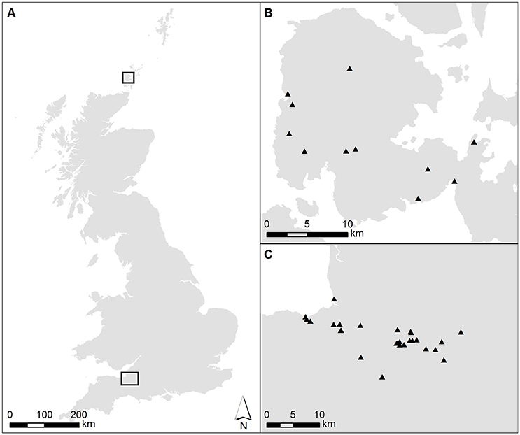
Figure 2. (A) Map of the UK, showing the location of the two case study areas, with insets outlining the study areas at a larger scale. (B) Orkney Mainland [upper box in part (A)]. (C) The Somerset Levels and Moors. Gray shading shows present-day dry land, white shows sea. Solid symbols show the locations of pollen records included in the MSA reconstructions (see Bunting et al., unpublished; Farrell et al., unpublished for more detail).
In contrast to the Somerset Moors and Levels, the landscape of Orkney is generally understood to have been largely or entirely treeless during the Neolithic (e.g., Davidson and Jones, 1985), though paleoenvironmental work suggests that occasional stands of woodland were present into the Bronze Age (Farrell et al., 2014). The wealth of Neolithic archaeological remains in Orkney also contrasts with the Somerset case study, with well-preserved settlements, tombs and monuments still dominating the landscape in many places even today. Recently developed chronologies for Neolithic archaeology (Griffiths, 2016; Bayliss et al., 2017) can be compared with land-cover reconstructions which were made for 200-year “timeslices” over the period 4200–2200 cal BC.
The Physical Environment
For both case studies, a DEM of modern surface elevations derived from Ordnance Survey PANORAMA DTM NTF geospatial data supplied by EDINA Digimap at a scale of 1:50,000 was used as a starting point for land-cover modelling. The NTF data were clipped to the spatial extent of the study area and converted to IDRISI format using the GridIn application (Middleton, unpublished). Surficial geology grids were prepared based on British Geological Survey SHAPE geospatial data provided by EDINA Digimap at a scale of 1:50,000 for Somerset and at a scale of 1:625,000 for Orkney. A simplified classification was created in ArcGIS 10.3.1 and converted to IDRISI format using the GridIn application (Middleton, unpublished). The basic grids had 50 × 50 m pixels, and covered 36 × 49 km for the Somerset Moors and Levels case study and 32 × 30 km for the Orkney case study (see Figure 2).
Both areas have been affected by sea-level change in the early and mid-Holocene, but paleogeographical reconstructions at suitable resolution are not available. In the Somerset Levels and Moors, published paleogeographic maps of Bridgwater Bay show profound changes during the early and mid-Holocene (Kidson and Heyworth, 1976; Long et al., 2002), but by the start of the Neolithic, most of the area of interest was free from marine influence, and current understanding suggests that the paleogeography was broadly the same as at present from around 4200 cal BC. We therefore used the present-day surficial geology maps (showing the distribution of peat, alluvium, and coastal sediments) as the main guide for the distribution of wetland communities. The position of the Orcadian coastline has changed significantly during the Holocene due to rising sea-levels, with its present position having been reached at c. 2000 cal BC (Wickham-Jones et al., 2016, 2017). Current understanding of Holocene sea-level change in Orkney largely relies on general models produced for North-West Europe (e.g., Sturt et al., 2013). Local sea-level data for Orkney is currently being produced (Dawson and Wickham-Jones, 2007; Bates et al., 2013), but at present chronological resolution is too coarse to allow for estimation of sea-level in 200-year timeslices, therefore in this study modern coastline position was used for all timeslices.
The Vegetation Communities and Their Distribution
The main pollen types found in diagrams from each region were used as the basis for simplified plant community definition based on literature and understanding of the ecology of each case study area (summarized in Table 1).
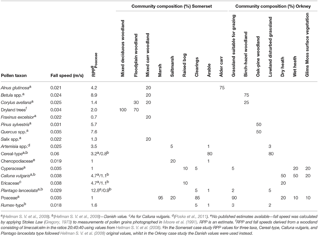
Table 1. Pollen dispersal and deposition model parameters and vegetation community compositions used in the pollen dispersal and deposition modelling.
In the Somerset Levels and Moors case study, placement of communities within the landscape assumed that vegetation could be divided into wetland and dryland areas, with saltmarsh, reed swamp and mudflats present in the western Levels where tidal influences dominated, floodplain and carr wet woodlands in the eastern Moors, and mixed deciduous woodland on the surrounding dryland and on raised burtle islands within the wetlands. Distribution of wetland communities is based on the modern surficial geology in all timeslices. Where peat is mapped as present, wet woodland was placed, and floodplain woodland was placed on areas of alluvium. In areas mapped as Holocene tidal sediment, beach deposits or sand, pixels were allocated to either bare mud, marsh or saltmarsh with a probability distribution of 0.2:0.4:0.4. All other land areas above 3 m asl were modelled as supporting mixed deciduous woodland. In the Orkney case study the landscape was modelled as a mosaic of birch-hazel woodland and grassland suitable for grazing animals. Areas of disturbed grassland, which could either occur naturally, for example in response to storm deposits of sand and/or salt, or due to anthropogenic activity, were placed below 30 m asl, and given a single community composition including low pollen production cereals, some bare ground and some high-pollen-producing weeds associated with disturbance (Artemisia-type, P. lanceolata and Rumex-type). Stands of pine and oak woodland were placed in sheltered, well-drained situations (slope >5°, altitude < 100 m, aspect E, SE, or S). The amount of woodland present was varied independently between “upland” (defined following Lamb, 1989 as land above 60 m asl) and “lowland” areas, since it is possible that anthropogenic clearance might have been greater in the lowlands, and edaphic processes and exposure might contribute more to woodland loss in the uplands. Local wetland vegetation at each coring site was inferred from the published records. Where data were insufficient to allow this multiple possibilities were tested during the early “scoping runs” (see section Pollen Assemblage and Radiocarbon Age Estimate Data below).
Pollen Assemblages and Chronologies
All available radiocarbon dated pollen records were collected, and new age-depth models constructed to ensure a common chronological framework. The age of each sample was determined as the median of the Highest Probability Density Interval and pollen data for all samples falling within a particular timeslice were summed and averaged to produce a single pollen assemblage at each location during each 200-year timeslice as the targets for reconstruction. Not all pollen sequences contained samples dating from every timeslice, so each timeslice uses a slightly different set of pollen records.
Scripts and Scripting/Workflow
For each landscape, initial scoping runs explored a wide range of possible levels of woodland cover and variations in local wetland structure, then more focused runs were carried out using a narrower range of vegetation options, which allowed for a larger number of repeats of each scenario and therefore better incorporation of random placement effects in outputs. For example, in the Somerset Levels and Moors, the scoping run assessed the fit for landscapes with clearings occurring in either just the dry land woodland or in all types of woodland, with the proportion of clearings in each woodland type ranging from 0 to 100% in 10% increments, and in addition at each coring point, local wetland vegetation was modelled as either marsh or raised bog within wet woodland, and marsh or raised bog with a surrounding ring of alder carr of varying width. The radius of the bog or marsh was varied in 50 m increments from 50 to 800 m, and the width of the surrounding alder carr was also varied from 50 to 750 m. In combination, this gave 512 different configurations for the local wetland vegetation and 22 woodland clearing configurations, generating 11,264 possible scenarios for each timeslice. For the Orkney case study, the first scoping run considered a very broad range of scenarios from a 100% open landscape to a 100% wooded landscape, along with different proportions of heathland, oak-pine woodland and disturbed ground. Later runs varied the structure of vegetation as well as the proportion of cover (e.g., whether woodland occurred as discrete patches or scattered pixels). The vegetation placement constraints used in the final scripts are described in section The Vegetation Communities and Their Distribution above, and multiple replicates of each scenario were run, since vegetation patches were placed randomly and pollen records are known to be sensitive to vegetation patterning as well as overall vegetation composition (Bunting et al., 2004).
Model Uncertainties
No model is a perfect reconstruction of a natural process, and the complexities of the pollen-vegetation relationship mean that the models used here are likely to be highly imperfect. Both the LRA and the MSA rely on the assumption that the dispersal and deposition model chosen is appropriate to the system being studied, and that the p.e. type properties of Relative Pollen Productivity and fall speed (see Supplementary Material) can be treated as constants for a given study location. Empirical measurements of these variables suggest that this is not a good assumption, and research is ongoing to improve understanding of the range of and controls on these variables (reviewed in detail elsewhere e.g., Mazier et al., 2012; Bunting et al., 2013) and the size of the errors introduced by variation.
Unlike the LRA, which treats all p.e. taxa individually, the MSA includes the option to group taxa into communities. Since the MSA produces a grid output rather than numerical, the pixel size of the grid acts as a limitation on the variability possible in the landscape. The landscape is conceived as a mosaic of communities, although p.e. taxa can be components of multiple communities. This is partly driven by concern over pixel size. Assigning each pixel to a single taxon allows each taxon to have different specified environmental constraints, and communities should emerge from the co-occurrence of types with similar ecological requirements at particular locations. However, this is only reasonable if the pixel size is comparable to the size of a vegetation unit, e.g., an individual tree or heather bush, or a grass tussock. Pixel size is determined by three factors: the available resolution of input data (although resampling can change the resolution of a grid, finer sampling risks introducing rounding errors), computer processing capacity and time available for analysis (more pixels means more calculation steps for each simulated pollen sample therefore longer run times for software), and thirdly the overall size of the landscape grid, since the HUMPOL approach of calculating values for each pixel and summing them across the landscape requires at least some rounding of values for holding in the computer memory, and the larger the grid, the greater the risk of introducing errors. Grid size in turn is determined by the spatial properties of pollen dispersal and deposition, since the MSA approach requires that the landscape considered includes most of the pollen source area of the sites sampled. There are many definitions of pollen source area, multiple factors that affect the value for different combinations of taxa, landscapes, site types, and pollen dispersal and deposition models chosen, and many estimates of its value, but there is general agreement that grids need to be large (at least 10 s of km) to capture some of the background component of the pollen rain. The 50 m pixel size chosen for these case studies was a compromise between these different factors, is larger than most individual trees, and can contain hundreds of thousands of individuals of herbaceous taxa.
For these case studies, we chose to assign each pixel to a community, which would allow us to explore the behavior of “indicator taxa” in the pollen record (distinctive p.e. taxa associated strongly with particular land uses or communities, but rarely present in great abundance). We defined community composition from field observation, evidence from regional pollen diagrams and ecological understanding; clearly the assumptions here are extensive and introduce uncertainties which are difficult to quantify (e.g., dryland woodland composition in Somerset will have been far more varied at multiple scales than was modelled here). One possible future approach might be to use REVEALS to reconstruct the proportion of each p.e. type in the entire landscape, and use those values to define the community compositions. These choices can also be refined by drawing on multiple lines of evidence (e.g., woodland composition could be estimated from trackway construction materials in the Somerset Levels), although these bring their own uncertainties into the analysis.
Over-complex models are not better models, and a balance between multiplying assumptions and achieving outputs of use to the intended research community needs to be struck. Clearly specifying the choices made, so that the user of model outputs can critically evaluate the results, is essential. Limiting the number of taxa to a very small group, where each taxon is representative of and largely confined to a distinctive land cover element, may be a viable alternative strategy, as shown by Nielsen and Odgaard's (2005) study of historic land cover in Denmark using four taxa, Poaceae (pasture), Calluna (heath), tree pollen (a composite taxon; woodland), and Cerealia (arable cultivation). Definition and quantification of uncertainties associated with MSA reconstructions is a challenging task for the future; in this paper, we focus on outputs expressed as trends and estimates of the extent of change, and use of output grids as hypotheses to be tested by designed collection of palaeoecological or other data.
Results
Results in the form of single best-fit land cover grids and summary landscape characters for each time slice were extracted as described above. Standardized overall fit scores (overall fit for the grid as a whole, divided by the number of sites included) for all these grids lie mainly between 20 and 30 (overall possible range of 0–200), mostly at the lower end, which modern sample comparison suggests is within the range of typical values when comparing modern pollen samples collected within the same broad vegetation communities (e.g., Lytle and Wahl, 2005). Standardized overall fit generally lies within the standard error of the mean of the individual site best fits, suggesting that the two different methods of summarizing land cover described in the methods (section Handling Output Data) are based on comparably good (or bad) reconstructions.
Reconstruction results are shown in Figures 3–6. Examples of good-fit land-cover maps for each timeslice from Orkney are given in Figure 3 and landcover proportion trends are plotted in Figure 4. Figures 5, 6 show the same data for Somerset.
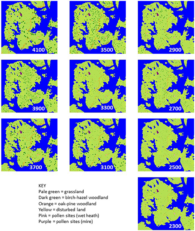
Figure 3. Example best-fit grids of land cover for Orkney case study in 200 year timeslices between 4200–2200 cal BC (age shown is midpoint of timeslice).
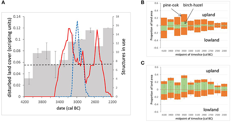
Figure 4. Trends in land cover extracted from MSA reconstructions for Neolithic Mainland, Orkney (axis labels in modelling units—see text for details). (A) Variation in disturbed land community presence below 30 m a.s.l. (dashed line marks baseline from timeslice pre-dating first substantial archaeological dating evidence in the studied area). Solid red line shows radiocarbon-derived activity estimates in the “peripheral” area, blue dashed line shows radiocarbon-derived activity estimates in the “core” area (see Farrell et al., unpublished for more information). (B) Tree cover modelled as discrete woodland stands—trends in the upland and lowland areas of the modelled landscape (above and below 60 m asl). (C) Tree cover modelled as scattered trees or small copses—trends in the upland and lowland areas of the modelled landscape (above and below 60 m asl).
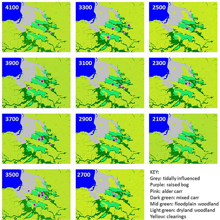
Figure 5. Example best-fit grids of land cover for the Somerset case study in 200 year timeslices between 4200 and 2000 cal BC (age shown is midpoint of timeslice).
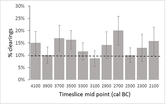
Figure 6. Changing proportion of clearings in the Somerset case study landscape in 200 year timeslices between 4200 and 2000 cal BC based on mean of the five best fit reconstructions identified through the MSA. Dashed line represents pre-Neolithic base-line conditions (see text for details).
Discussion
Here we consider what MSA reconstructions offer in terms of understanding the Neolithisation of the contrasting case study landscapes, then briefly discuss issues arising from this first full application of the MSA as a reconstruction tool and explore possible remedies, before evaluating the potential place of the approach within main-stream palynological research.
Landscapes of Neolithisation
Orkney: Neolithisation in a Largely Treeless Landscape
In the Orkney case study, pollen records came from discrete wetlands scattered across the landscape. Some sites consistently yielded lower fit scores than others, at least partly due to uncertainty about the nature of the local wetland vegetation at the pollen sites. The characteristics of some study sites (e.g., Hobbister—Farrell, 2015) were clearly changing during the study period, and full investigation and mapping of the stratigraphic units and hence former sedimentary environments to support better reconstruction is not always possible (e.g., due to active peat extraction at Hobbister).
“Plausible” (sensu Caseldine and Fyfe, 2006) mapped land-cover reconstructions for all 10 timeslices across the period 4200–2200 cal BC are shown in Figure 3 and land-cover trends plotted in Figure 4, compared with the intensity of settlement activity in “core” and “peripheral” areas across Orkney derived from the number of dated structures in use on individual sites (Figure 4A; Bayliss et al., 2017). A baseline for disturbed grassland communities in the pre-Neolithic landscape (communities with higher proportions of anthropogenic indicator taxa than the “natural” grassland) can be taken from the timeslice 4200–4000 cal BC. At this point c. 12% of the landscape was wooded, mainly birch-hazel. Less than 1% of the study area was made up of the “disturbed grassland” community.
The first dated archaeological evidence of settlement in Mainland Orkney is recorded during the 3600–3400 cal BC timeslice (Bayliss et al., 2017). The increase in dated settlement activity, particularly in the “core” Brodgar-Stenness area, over the period 3200–2800 cal BC is associated with a significant increase in inferred landscape disturbance. The subsequent decline in dated structures in both “core” and “peripheral” areas of Mainland is not associated with a reduction in cover of the disturbed grassland community, which actually increases in the 2800–2600 cal BC timeslice, following abandonment of the “core” area of Neolithic activity, and the 2400–2200 cal BC timeslice, following abandonment of settlements in the “peripheral” area of Mainland.
Established Neolithic activity on Mainland Orkney probably began in the thirty-fifth century cal BC (Bayliss et al., 2017; Bunting et al., unpublished), about 300 years later than elsewhere in Britain and Ireland (Whittle et al., 2011), implying that Neolithic people were slow to establish themselves on Mainland. The MSA reconstructions support this relatively late start date. Prior to any dated Neolithic activity, the landscape was dominated by grassland suitable for pasture. This natural prevalence of grassland may help to explain the rapid expansion of Neolithic settlement on Mainland, since the Neolithic Orcadian economy probably relied heavily on cattle (see Mainland et al., 2014; Card et al., 2017) and extensive clearance would not have been necessary to provide land for grazing. Inferred variations in the amount of “disturbed ground” above the baseline from the 4000 to 3800 cal BC timeslice onwards may hint at earlier anthropogenic disturbance by either late hunter-gatherers or farming pioneers; Sharples (1992) has suggested that the comparatively heavy soils on Mainland Orkney were exploited later than other islands.
A distinct shift in land-cover is reconstructed between 3400 and 3000 cal BC (see Figure 4), the period that covers the first sustained tomb building, the shift from timber to stone houses, and the concentration of settlement in the “core” Brodgar-Stenness area of Mainland (Bayliss et al., 2017; Bunting et al., unpublished). There is an increase in coverage of the “disturbed ground” community and a reduction in woodland cover, but woodland does not disappear from the landscape entirely. Woodland would have been a valuable resource for Neolithic Orcadians (Farrell et al., 2014), and was already scarce (Figures 3, 4) at the time of the first dated settlement activity (3600–3400 cal BC timeslice), and falls by around 50% between the 3400–3200 cal BC timeslice and the 3200–3000 cal BC one, suggesting that some loss of woodland occurred with the first dated Neolithic activity in the area. The clear coincidence between changes in land cover and settlement occupation, dated using the same age model construction approach but independent sets of radiocarbon dates, suggests that land cover reconstruction using the MSA may provide a proxy for settlement activity even in landscapes where impacts are expected to have been small scale.
A decline in settlement activity in the Stenness-Brodgar “core” area in the 2800–2600 cal BC timeslice does not coincide with any reduction in potentially cultivated “disturbed ground” or with woodland regeneration in the MSA reconstructions; human population may have become dispersed into smaller settlement units, away from the socially unsustainable concentrations of people in the major Neolithic complexes of the Stenness-Brodgar peninsula, rather than actually reducing in size. A further decline in woodland coverage is seen in the last two time-slices, coinciding with the time activity was re-established in the “core” area in the twenty-sixth century cal BC. These MSA reconstructions also contribute to understanding the end of the Neolithic in Orkney. Several possible reasons for the decline of the Grooved Ware culture have been proposed (see Clarke et al., 2018, for a review), including environmental stress and climatic deterioration (cf. Meller et al., 2015). The reconstructions presented here do not show the changes in land-cover which might be expected to accompany a climatic downturn (e.g., spread of acid heathland), nor do they provide evidence for abandonment. This suggests continuity of land-use, and it seems more likely that the cause of the Grooved Ware decline has its root in social factors rather than environmental deterioration (Farrell, 2009; Bunting et al., unpublished). This interpretation supports Downes (2005) suggestion that the apparent scarcity of Bronze Age settlements in Orkney is probably the result of failure to identify them rather than a true lack of occupation.
Even at the time of most intensive dated settlement activity in the 3200–3000 cal BC timeslice, the “disturbed” community accounts for only around 4% of available land (from the landscape-scale reconstruction: see section Handling Output Data above), although anthropogenic activity is also the most likely cause of the observed woodland cover decline. Many classic anthropogenic indicator plants were already present as part of the grassland community, and would also have existed in naturally disturbed habitats close to the coast; consequently increases in these indicator taxa and changes in composition of open vegetation communities have a much more subtle palynological signal compared with reductions in tree pollen. Figure 4 shows how the quantification of changes made possible by applying the MSA allows us to draw out this relatively subtle signal and compare it with the archaeological record.
Differences in woodland coverage in Orkney above and below the 60 m asl limit of prehistoric cereal cultivation are illustrated in Figure 4B (tree cover modelled as woodland patches) and Figure 4C (tree cover modelled as scattered trees). The results clearly illustrate the equifinality associated with MSA reconstructions. Where trees are modelled as patches of woodland (Figure 4B), woodland cover is generally similar in both upland and lowland areas, and the more diverse woodland incorporating oak and pine tends to be more abundant than the pure birch-hazel “scrub” community. Where scattered trees are modelled (Figure 4C), the upland areas tend to contain more woodland than the lowlands, and the more diverse woodland is more abundant in the lowlands. This second option is perhaps more realistic from an ecological point, but the two sets of scenarios cannot be distinguished on the basis of the existing pollen records.
These outputs can be used to identify pollen sites for future studies designed to test these two contrasting hypotheses for former woodland distribution, by taking pollen records from small basins whose pollen source area lies above or below the 60 m asl limit and comparing pollen assemblages across the study period at an appropriate sampling interval (e.g., 100–200 years, comparable with the reconstruction) to determine whether there is a systematic difference in woodland coverage or not. The modelling approach used here assumes that all pollen at the target sites originates from within the modelled area of Mainland. Certainly for pine, a long-distance component from Hoy and Northern Scotland will also have formed part of the target pollen assemblages, although simple “thought experiment” modelling suggests that non-Orcadian sources contribute < 20% of the total pine pollen recorded. This component may partly explain the apparent stability of oak-pine woodland coverage in comparison with the variation in coverage of the birch-hazel community. A relatively small number of target pollen sites are included in any single timeslice, and the differences in which sites are included in each timeslice are also likely to contribute to the variability seen in the reconstructed land-cover, but the overall patterns provide some more detail on the likely location of woodland in Neolithic Orkney.
Somerset: Neolithisation of a Densely Wooded Landscape
Examples of good-fit land-cover maps for each timeslice in the Somerset case study area are given in Figure 5 and landcover proportion trends are plotted in Figure 6. The start of the Neolithic in this area occurs during the 3800–3600 cal BC timeslice (see Farrell et al., unpublished) and the 4000–3800 cal BC timeslice is used to define the pre-Neolithic landscape. The initial openness level of c. 10% is presumably due to natural processes such as wind-throw, lightning strikes and grazing by wild herbivores (Brown, 1997). The higher level of clearings implied for the earlier 4200–4000 cal BC timeslice is assumed to reflect the response of land cover to the end of a phase of falling relative sea-level, as the lower-lying parts of the Levels and Moors become wooded. The proportion of woodland clearings within the timeslices 3800–3600 and 3600–3400 cal BC rises, which is interpreted as anthropogenic clearance of woodland in the wider landscape. Between 3400 and 2800 cal BC, the standard errors of estimated clearance overlap with the baseline clearance level, which is interpreted as a reduction in the extent of human-related woodland openings; in two of these three timeslices the mean is still above the 10% baseline. For 2800–2600 cal BC, clearings increase to c. 20% of the potential woodland area, interpreted as an increase in landscape modifying human activity. The proportion of cleared land then falls back to approximate baseline between 2600 and 2200 cal BC, and rises to around 16% in the final timeslice (2200–2000 cal BC).
MSA land-cover reconstruction shows that at times the proportion of cleared land increases to 50–100% above the pre-Neolithic baseline, which is interpreted as reflecting additional disturbance of the woodland due to anthropogenic clearance. Some of these clearances may result from woodland management, since coppiced wood was used in the construction of Neolithic trackways in the region (Coles and Coles, 1986, 1992), and others may be associated with agricultural activity on the dryland such as small-scale cultivation or management of grazing animals. These results may be taken as a kind of proxy settlement record in an archaeological landscape that currently lacks evidence for occupation sites, allowing some preliminary comparisons and contrasts to be drawn with neighboring regions. The suggestion of initial activity in the thirty-ninth century cal BC conforms with the wider picture for the beginning of the Neolithic proposed by Whittle et al. (2011), and increased woodland clearance between 3800 and 3400 cal BC corresponds with the scale of monument construction seen in southern Britain during this time. The reduction in clearance seen in the 3200–3000 cal BC timeslice is also of interest, given recent debate about possible discontinuity of cereal cultivation in the later fourth millennium cal BC (Stevens and Fuller, 2012). Decreased activity in the 2600–2400 cal BC timeslice serves as a valuable reminder of regional variation at a time when major constructions and cultural changes were taking place in the Stonehenge area.
Future modelling-supported research questions to be explored in the Somerset area include investigating the location of early human activity in this landscape complex. In this analysis, woodland disturbance could occur anywhere with equal probability, but prehistoric human populations are known to use different parts of landscapes differently. Modelling could be used to determine whether it is possible to separate a pollen signal from human activity focused around the Levels and Moors on one or more wetland margin settings, river margins, or burtle islands and the Polden Hills from activity spread more widely in the landscape, using archaeological understandings of Neolithic landscape utilisation to inform the “rules” which control possible location of clearings, and to explore the effects of different models of landscape utilisation on the pollen signal (through different lengths of cropping, fallow/grazing, and woodland successional phases). In future archaeological research programmes, the reconstructions presented can be used as a starting point for identifying the coring locations most likely to produce pollen records which include archaeological sites of interest within their source areas, and thereby improve the integration of the two methodologies.
Evaluation of the Reconstruction Approach
The studies reported here are the first full implementation of the MSA for reconstruction of past land cover from pollen records, therefore it has brought both strengths and weaknesses into clear focus. Discussion is organized around the stages of reconstruction.
Input Data
The MSA incorporates landscape characteristics overtly in the reconstruction of past land cover, which improves the plausibility and usefulness of the output, but depends on being able to clearly define these characters. Topographical (DEMs) and geological data are readily available in mapped forms for the UK, and at the temporal and spatial scales used can be considered invariant. Palaeogeography proved more challenging, as sea level and the distribution of water bodies are known to have changed during the Holocene substantially enough to affect the reconstructions. In both case studies, after consulting all available evidence, we decided to assume the coastline was in its modern position, and in Orkney it was also assumed that extant lochs were in the same size and position, and that no loss of water bodies through drainage or hydroseral succession had occurred. These assumptions are clearly wrong, but how to improve them without introducing additional sources of uncertainty was not obvious.
Reconstructing paleo sea level, paleo coastal geomorphology and paleo landscape hydrology is a non-trivial exercise. For the Somerset case study, we were able to access a reconstruction of paleogeography which used a basemap derived from Sturt et al. (2016; see SI3 in Farrell et al., unpublished for details). However, translating this into pre-Neolithic coastline position and identifying areas subject to marine influence would also require reconstruction of sediment infilling across this landscape from coastal, fluvial, and hydroseral processes, and whilst sediment stratigraphy and dating evidence do exist for much of the area which could form the basis for such an exercise, it was beyond the scope of the present study. By allowing for a wide range of local wetland conditions at the coring points (combinations of mire, marsh and alder carr in Somerset, and of mire and marsh in Orkney) in the scoping runs the MSA was able to incorporate some of the variation in wetland conditions that would have resulted from changing sea level and paleogeography in both case studies and therefore reduce the impact of incomplete knowledge of past coastline. Some sites used as targets in both case study areas are in locations where paleogeographical changes could have made a large difference to the landcover within a few hundred metres of the basin edge, and where such sites are identified they could be downweighted when identifying the quality of fit of the overall reconstruction. In both our case studies, reconstructed land cover from such sites was close to that from sites without such influences, showing that all sites were picking up a comparable regional pollen signal and such down weighting would not change the outcomes substantially.
An unanticipated problem was the difficulty of accessing data for published pollen records, and in some cases values had to be “read” from published diagrams rather than using original counts, showing the challenges of maintaining access to data over the longer term.
Specification of Land Cover Units
After identifying the main pollen taxa (palynological equivalent types, as discussed in section Model Uncertainties above), the next step is to decide what land cover units will be used in the reconstruction. For these case studies, 50 × 50 m pixels were used and land cover was specified as communities (see section Model Uncertainties above). Using communities as land cover classes does enable us to include the pollen signal from “indicator taxa” such as P. lanceolata in the analysis, but the problem of defining past community composition is particularly apparent in the Orkney case study. A single disturbed ground community was used, including low pollen production cereals, some bare ground and some high-pollen-producing weeds associated with disturbance (Artemisia-type, P. lanceolata and Rumex-type). Future work should clearly use at least two disturbance communities, with and without cereals present, but the run time available in the project reported here did not allow us to start again once this became apparent—adding an extra community to the analysis increases the run time for analysis almost two-fold. All the taxa involved are present at low abundance in the target pollen signal, so the results of re-analysis are not expected to change the interpretations presented here.
Over-complex models are not better models, and a balance between multiplying assumptions and achieving outputs of use to the intended research community needs to be struck. One approach for future testing may be to reduce the number of taxa to a very small group, where each taxon is representative of and largely confined to a distinctive land cover element, as shown by Nielsen and Odgaard's (2005) study of historic land cover in Denmark using four taxa, Poaceae (pasture), Calluna (heath), tree pollen (a composite taxon; woodland), and Cerealia (arable cultivation).
A strength of the MSA over other reconstruction approaches is that it is possible to overtly include local wetland vegetation in the reconstructions. Identifying the pollen rain component sourced from “local” or “extra-local” vegetation (sensu Janssen, 1984) is a common concern in pollen record interpretation. One approach is to select sites where such vegetation can easily be identified and excluded (e.g., lakes—obligate aquatic plant pollen can be excluded—or ombrotrophic Sphagnum mires with minimal vascular plant vegetation). However, nature rarely obliges in the availability and distribution of such sites, and especially in lowland areas wetlands of many types are the main or only sources of pollen data. On-site vegetation contributes to the pollen signal in multiple ways (Bunting, 2008), which can obscure the signal of the upland landscape. Some scientists, especially for studies where data from multiple paleoecological proxies are available, take considerable pains to first reconstruct the wetland vegetation and then consider the surrounding dry land, whereas in other cases and in most multi-site synthesis studies local vegetation contributions are treated as “noise” or otherwise ignored. Interest in the variety and complexity of sedimentary systems which preserve pollen records was one of the incentives to develop the MSA. In the LRA, wetland vegetation must be removed or ignored (by either removing possible wetland taxa such as Cyperaceae, or assuming that the contribution of on-site taxa to the pollen record is negligible) which can restrict the selection of sites to those where the assumption of negligible input is most reasonable, e.g., lakes or pure Sphagnum mires. For the many landscapes where lake sites or ombrotrophic mires which are effectively pure Sphagnum lawns are not available to act as sources of pollen records, this ability to not just consider but address the potential concerns is a clear strength of the MSA over other reconstruction methods.
Both case studies demonstrate how the MSA can overtly address the issues of local site vegetation. Including variation in the size and type of on-site vegetation was an important part of the scoping stage for both case studies. In the Somerset case, pre-existing data about site stratigraphy which might inform interpretation was not easily available, so a strategy of very wide scoping of options was used. This allowed us to identify a single range of conditions which led to the lowest best fit scores, which we assumed for efficiency represented a reasonable reconstruction of the local wetland conditions, and then used in further analysis. In the Orkney case, determining local vegetation was more straightforward since sites were discrete entities and a combination of geomorphological limits with published stratigraphic data and site reconstructions allowed us to assign broad community types to each wetland. In some cases multiple good-fit sets of conditions were identified during scoping. Figure 7 shows an example from Somerset, where site WLT has two possible wetland configurations producing good fits, a moderate-sized mire with no alder carr fringe in a landscape with levels of clearing between 0 and 40% or a mire of variable size with an alder carr fringe 500–550 m wide in a landscape with about 20% clearings during the scoping process. For expediency, the set with the overall lowest fit score was used in further analysis, but a fuller study would either explore other data to test which was the more plausible alternative (sensu Caseldine et al., 2008) or run the further analyses with both options to avoid cutting off possible solutions. Hydroseres are spatially as well as temporally variable and the complexity of surface arrangement of palynologically distinct wetland communities in extensive peatlands can be considerable (Waller et al., 2005, 2017). Reconstructing this complexity in the past is challenging, requiring extensive coring work for robust results, but is increasingly included in new studies of hydroserally complex sedimentary sequences.
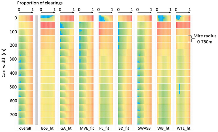
Figure 7. Example of equifinality in Multiple Scenario Approach outputs: Somerset case study scoping run for the 4400–4200 cal BC timeslice (not presented in Figure 5). Comparison of fit scores summed across the landscape (overall) and for eight individual sites (see Farrell et al., unpublished for details) for scenarios where each coring point is modelled as an area of mire surrounded by an alder carr belt, and mire size, carr width and proportion of clearings in the wider landscape are all varied. Colour shows relative fit score value for each dataset (single column, 2,816 scores), where green is low and red is high. The lowest 2% of values (identifying the scenarios which produce simulated pollen assemblages most similar to the actual pollen recorded) are highlighted with blue overlay.
Future Developments
Four main strengths of the approach are identified. First, the MSA allows the analyst to overtly incorporate wetland vegetation (discussed in Specification of Land Cover Units above) and changing wetland conditions into the reconstruction, rather than avoiding or ignoring the potential complications. Secondly, the MSA is suitable for reconstruction of land cover where the assumption of uniform vegetation within the “region” (e.g., within 50–100 km radius of the studied sites), required by the LRA for reconstruction of vegetation detail at a 1–2 km level from small pollen sites, is clearly problematic. This opens up many more landscapes to possible reconstruction, including much of the UK. Thirdly, the MSA package makes landscape specific “thought experiment” type approaches which incorporate known landscape constraints relatively easy to carry out (e.g., Caseldine et al., 2007). Finally, the MSA also encourages the analyst, and potential end users of paleoecological data who may not have the detailed understanding of the complexities, limitations, and uncertainties of analysis outputs, to be more aware of equifinality. Paleoecological data offer a “muddy time machine,” an invaluable insight into past ecologies and landscapes, but the view out of the window is obscured and fragmentary. Identification of a range of possible reconstructions moderates the tendency to tell a good story as if it is the only possible reconstruction of a landscape, and creates natural hypotheses for future testing, thus contributing to the ongoing challenge of improving the level of scientific reasoning in paleoecological circles.
There remains considerable challenge in communicating uncertainty in a visual way. One option might be to add together all the grids satisfying the fit threshold and create maps of the probability of a land cover type being present at a given pixel across all the grids. We expect that greater confidence in reconstruction would be found close to sites, within the zone which is sensitively recorded by the pollen assemblages, and lesser confidence with increasing distance from the sites. It is important that results are communicated to end users in ways which emphasise that these are hypotheses, and the use of the models to identify ranges of probable past land cover characters (e.g., Gillson and Duffin, 2007), rather than a single “correct” reconstruction.
Direct outputs from LandPolFlow are in the form of a.csv file of simulated pollen loadings, model parameters, and fit scores, and in the form of grids showing mapped land cover. In this paper we have presented sample grids and summaries based on model parameters which produced the best fit scores, but there are multiple other ways of presenting the output, and developing strategies for effective communication of results is an important area of model development for future attention.
Maps are visually appealing and striking, and the ease of choosing a single best-fit map as the reconstruction makes it a tempting solution, but one which doesn't make full use of the information provided by the MSA. For these case studies we mostly worked with a small number of scenarios with the lowest scores, largely due to resource restrictions, but for future projects analysis should logically take into account all scenarios with fits below a pre-defined threshold. That will require the analyst to set a threshold (using e.g., consideration of the sampling effects within count data, or criteria derived from modern studies of samples from different communities such as Lytle and Wahl, 2005). In some runs a large number of scenarios may produce fits below the threshold, but this diversity could be reduced by using model parameters to identify which families (groups of scenarios with the same environmental constraints repeated so that probabilistic elements such as patch placement vary), and how many members of each family, are present. Each family may represent an equifinal reconstruction option.
A method of further choosing amongst possible reconstructions is to consider their plausibility. Caseldine et al. (2008) argued that to be considered a reconstruction, a scenario should not just be capable of producing a simulated pollen signal which is statistically similar to the actual data, but should also be capable of being linked temporally with landcover arrangements (maps) which pre-date and post-date it, through reasonable ecological processes and patterns of change. Within this study, an example of a reconstruction which was a good fit but not plausible was obtained for the Orkney 2800–2600 cal BC timeslice, when several of the best-fit grids were from scenario families with 10% of the area above 60 m asl supporting heathland. Reconstructions for timeslices both before and after did not include any options with heathland present, and development of heathlands in the uplands is usually a progressive process. Therefore we deemed the reconstruction implausible, and used the land cover grid with the best fit and no heathland for the reconstruction sequence. In this case, we believe that the implausible scenario was reflecting variation in the on-site vegetation in one or more of the sites included for that timeslice.
In the case studies presented here, each time slice was treated individually, in order that a problem in one time slice would not be propagated into others, and could more easily be detected as an anomaly. An alternative way to use the MSA is to work on timeslices sequentially, beginning each timeslice with one or more grids from the best-fit family for the previous timeslice, and modifying the vegetation until suitable reconstructions are identified. This would ensure a plausible sequence, but would need to be carefully planned and carried out to avoid missing out on equifinal solutions along the way.
As an alternative to maps, results can be presented quantitatively, as landscape metrics. Examples here showed metrics taken from the output file, based on the model parameters of the best fit scenarios (e.g., the mean and standard deviation of the probability that a pixel in a defined landscape setting could be occupied by oak-pine woodland), which are not the same as land cover metrics (due to the random nature of land cover map creation). The trends they show can be interpreted with confidence, but the absolute values will not be accurate. Values of area of landscape occupied by a given community can be extracted directly from the land cover grids, and are a more attractive metric for end users, but at present are also far more labor-intensive to obtain. Improving the extraction of information from grids is a development priority for the MSA.
The MSA and the Palynological Workflow
Whilst the LandPolFlow package is complete and documented, the use of the MSA is in its infancy and not all package features are considered here. A suggested workflow for future studies is shown in Figure 8 based on our experience with these case studies, and Figure 9 shows how the methods could be built into palynological studies more generally. For these case studies we used R to speed up the manipulation of output files, and see considerable potential to use automation to increase the capacity of the method. More detailed validation of the MSA using modern pollen and vegetation datasets, currently under way, will also help understand its capacity and limitations better, and improve its deployment.
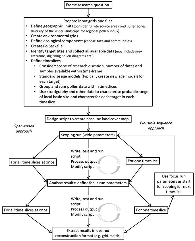
Figure 8. Recommended workflow for reconstruction of past land cover using the Multiple Scenario Approach (MSA).
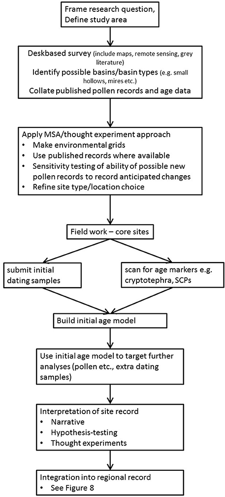
Figure 9. Recommended workflow for pollen analysis based investigation of past vegetation dynamics integrating the Multiple Scenario Approach (MSA).
As more sets of pollen dispersal and deposition parameters are published for different taxa and geographic areas, and as increasing processor speed reduces the time and computational resource needed to run LandPolFlow, we believe that modelling approaches should become a routine part of the pollen analysts' tool kit, as zonation using a constrained clustering approach such as CONISS rather than merely visual inspection has become routine since its introduction (Grimm, 1987).
Conclusion
Modelling approaches such as the MSA offer a clear route to getting more information from existing published pollen records, which represent a huge investment of time and money. This paper presents two case studies of the MSA in use at a landscape level, filling the gap between the regional land cover reconstructions offered by REVEALS (Sugita, 2007a; 100 × 100 km squares in e.g., Trondman et al., 2015) and the single-site reconstruction of distance-weighted plant abundance made possible by LOVE (Sugita, 2007b; distance of c. 500 m−2.5 km depending on site-specific Relevant Source Area of Pollen), and generating reconstructions in forms which are both transparent and useful for a wide range of end users, whether paleoecologists, environmental archaeologists, conservation biologists, neoecologists, or science communicators. The land cover hypotheses produced by the MSA can serve as the starting point for more structured, hypothesis-testing uses of paleoecology and environmental archaeology methods, including not only pollen analysis but also other techniques recording different aspects of land cover.
Our reconstructions of Neolithisation in both a heavily wooded and a largely treeless landscape show that, although the extent of land cover modification was limited and did not alter the essential character of each landscape, it was persistent. In Orkney, the timing of land cover change occurred at the same time as the start of settlement use as determined from an independent set of radiocarbon dates from archaeological sites, strongly supporting our interpretation of land cover change as a proxy for human activity in the wider landscape in the Somerset case study where archaeological evidence for Neolithic settlement is minimal. Increased levels of clearance or disturbance in both locations persisted even when archaeological evidence implied a reduction in intensity of landscape use and occupation, suggesting a significant transition in landscape character and ecology occurred with Neolithisisation. Modelling, and its ability to support targeted selection of sites for pollen analysis in specific environmental contexts and to address specific archaeological questions, clearly has a useful role to play in improving our understanding of landscape impacts and development, and in fostering better collaboration between paleoecologists and other disciplines concerned with past landscapes.
We argue that the MSA deserves a place within the pollen analyst's standard tool kit (Figure 9). There is still work to do in improving the use of the approach and the communication of outputs, and as with all models, outputs are dependent on assumptions and calibration and therefore “wrong” in an absolute sense. The case studies presented here show how LandPolFlow makes environmentally informed reconstruction of land cover accessible to pollen analysts, and therefore has the capacity to improve research design, prompt more overt, and thoughtful exploration of assumptions and site taphonomy, and improve communication between subject specialists and with wider stake holders.
Author Contributions
MB and MF: worked together on designing model strategy, iterative analysis of output of each run, interpretation of findings, and led the authoring of paper. MF: prepared input GIS grids, collated pollen targets, and carried out most model runs. PM: collated datasets and modelled radiocarbon chronologies for allocation of samples to timeslices with AB. PM, AB, and AW: selected sites in light of archaeological relevance and contributed to hypothesis development and output interpretation and representation.
Funding
This study was supported as part of The Times of Their Lives project (www.totl.eu), funded by the European Research Council (Advanced Investigator Grant 295412) and led by AW and AB.
Conflict of Interest Statement
The authors declare that the research was conducted in the absence of any commercial or financial relationships that could be construed as a potential conflict of interest.
Acknowledgments
First and most significantly, we wish to acknowledge the work of Richard Middleton. Now retired and busy with other projects (e.g., as Vice County Recorder of Botany for VC 61), he did not choose to be a co-author of this manuscript, but without his talent, enthusiasm, and willingness to explore unfamiliar intellectual territory this paper, and the wider MSA project, would never have come to fruition. We next acknowledge the many researchers who contributed pollen count data to the Somerset case study. We also wish to acknowledge the many members of the PolLandCal and LandClim networks, and of the PAGES Landcover 6k Working Group, for fruitful discussion of land cover reconstruction. We consider this work to be in part a contribution to the work of the PAGES Landcover 6k Working Group (http://www.pages-igbp.org/ini/wg/landcover6k/intro), included as part of the Past Global Changes (PAGES) project, which in turn received support from the US National Science Foundation and the Swiss Academy of Sciences. We thank two reviewers for comments on an earlier version of the manuscript.
Supplementary Material
The Supplementary Material for this article can be found online at: https://www.frontiersin.org/articles/10.3389/fevo.2018.00036/full#supplementary-material
Footnotes
1. ^ Plant species organized into groups on the basis of identifiability of their pollen grains; some types can be identified to species level e.g., Plantago lanceolata, whilst others can only be identified to genus e.g., Betula or family e.g., Brassicaceae, and some pollen types do not map neatly onto plant taxonomic groups (see e.g., Bennett K. D., 2007).
References
Bates, M. R., Nayling, N., Bates, R., Dawson, S., Huws, D., and Wickham-Jones, C. (2013). A multi-disciplinary approach to the archaeological investigation of a bedrock-dominated shallow marine landscape: an example from the Bay of Firth, Orkney, U. K. Int. J. Nautical Archaeol. 42, 24–43. doi: 10.1111/j.1095-9270.2012.00360.x
Bayliss, A., Marshall, P., Richards, C., and Whittle, A. (2017). Islands of history: the late neolithic timescape of Orkney. Antiquity 91, 1171–1188. doi: 10.15184/aqy.2017.140
Beckett, S. C., and Hibbert, F. A. (1978). The influence of man on the vegetation of the Somerset Levels - a summary. Somerset Levels Pap. 4, 86–89.
Bennett K. D. (2007). Catalogue of Pollen Types. Available online at: http://chrono.qub.ac.uk/pollen/pc-intro.html#introduction (Accessed November 17, 2017).
Bishop, R. R., Church, M. J., and Rowley-Conwy, P. A. (2015). Firewood, food and human niche contruction: the potential role of Mesolithic hunter-gatherers in actively structuring Scotland's woodlands. Quat. Sci. Rev. 108, 51–75. doi: 10.1016/j.quascirev.2014.11.004
Brown, A. (1997). Clearances and clearings: deforestation in mesolithic/neolithic Britain. Oxf. J. Archaeol. 16, 133–146. doi: 10.1111/1468-0092.00030
Bunting, M. J. (2008). Pollen in wetlands: using simulations of pollen dispersal and deposition to better interpret the pollen signal. Biodivers. Conserv. 17, 2079–2096. doi: 10.1007/s10531-007-9219-x
Bunting, M. J., and Farrell, M. (2017). Seeing the wood for the trees: recent advances in the reconstruction of woodland in archaeological landscapes using pollen data. Environ. Archaeol. doi: 10.1080/14614103.2017.1377405. [Epub ahead of print].
Bunting, M. J., Farrell, M., Broström, A., Hjelle, K. L., Mazier, F., Middleton, R., et al. (2013). Palynological perspectives on vegetation survey: a critical step for model-based reconstruction of quaternary land cover. Quat. Sci. Rev. 82, 41–55. doi: 10.1016/j.quascirev.2013.10.006
Bunting, M. J., Gaillard, M.-J., Sugita, S., Middleton, R., and Broström, A. (2004). Vegetation structure and pollen source area. Holocene 14, 651–660. doi: 10.1191/0959683604hl744rp
Bunting, M. J., and Middleton, D. (2005). Modelling pollen dispersal and deposition using HUMPOL software, including simulating windroses and irregular lakes. Rev. Palaeobot. Palynol. 134, 185–196. doi: 10.1016/j.revpalbo.2004.12.009
Bunting, M. J., and Middleton, R. (2009). Equifinality and uncertainty in the interpretation of pollen data: the multiple scenario approach to reconstruction of past vegetation mosaics. Holocene 19, 799–803. doi: 10.1177/0959683609105304
Card, N., Mainland, I., Timpany, S., Towers, R., Batt, C., Bronk Ramsey, C., et al. (2017). To cut a long story short: formal chronological modelling for the Late Neolithic site of Ness of Brodgar, Orkney. Eur. J. Archaeol. doi: 10.1017/eaa.2016.29. [Epub ahead of print].
Caseldine, C., and Fyfe, R. (2006). A modelling approach to locating and characterising elm decline/landnam landscapes. Quat. Sci. Rev. 25, 632–644. doi: 10.1016/j.quascirev.2005.07.015
Caseldine, C., Fyfe, R., and Hjelle, K. (2008). Pollen modelling, palaeocology and archaeology: virtualisation and/or visualisation of the past? Veg. Hist. Archaeobot. 17, 543–549. doi: 10.1007/s00334-007-0093-y
Caseldine, C., Fyfe, R., Langdon, C., and Thompson, G. (2007). Simulating the nature of vegetation communities at the opening of the Neolithic on Achill Island, Co. Mayo, Ireland — the potential role of models of pollen dispersal and deposition. Rev. Palaeobot. Palynol. 144, 135–144. doi: 10.1016/j.revpalbo.2006.07.002
Clarke, D. V., Sheridan, A., Shepherd, A. N., Sharples, N. M., Armour-Chelu, M. J., Hamlet, L., et al. (2018).“The end of the world, or just ‘Goodbye to all that'? Contextualising the late 3rd-millennium cal BC deer heap at Links of Noltland, Westray, Orkney,” in Proceedings of the Society of Antiquaries of Scotland, Vol. 146, 57–89. doi: 10.9750/PSAS.146.1226
Coles, B., and Coles, J. (1986). Sweet Track to Glastonbury. The Somerset Levels in Prehistory. New York, NY: Thames and Hudson.
Davidson, D. A., and Jones, R. L. (1985). “The environment of Orkney,” in The Prehistory of Orkney, ed C. Renfrew (Edinburgh: Edinburgh University Press), 10–35.
Dawson, S., and Wickham-Jones, C. R. (2007). Sea-level change and the prehistory of Orkney. Antiquity 81:312.
Downes, J. (2005). Cremation Practice in Bronze Age Orkney. Unpublished Ph.D. thesis, University of Sheffield.
Edwards, K. J., Fyfe, R. M., and Jackson, S. T. (2017). The first 100 years of pollen analysis. Nature Plants 3, 1–4. doi: 10.1038/nplants.2017.1
Eklöf, M., Broström, A., Gaillard, M.-J., and Pilesjö, P. (2004). Openland3: a computer program to estimate plant abundance around pollen sampling sites from vegetation maps: a necessary step for calculation of pollen productivity estimates. Rev. Palaeobot. Palynol. 132, 67–77. doi: 10.1016/j.revpalbo.2004.04.005
Farrell, M. (2009). The Environmental Context of Later Prehistoric Human Activity in Orkney, Scotland. Unpublished Ph.D. thesis, University of Hull.
Farrell, M. (2015). Later prehistoric vegetation dynamics and Bronze Age agriculture at Hobbister, Orkney, Scotland. Veg. Hist. Archaeobot. 24, 467–486. doi: 10.1007/s00334-014-0507-6
Farrell, M., Bunting, M. J., Lee, D. H. J., and Thomas, A. (2014). Neolithic settlement at the woodland's edge: palynological data and timber architecture in Orkney, Scotland. J. Archaeol. Sci. 51, 225–236. doi: 10.1016/j.jas.2012.05.042
Gaillard, M.-J., Sugita, S., Bunting, M. J., Middleton, R., Broström, A., Caseldine, C., et al. (2008). The use of modelling and simulation approach in reconstructing past landscapes from fossil pollen data: a review and results from the pollandcal network. Veg. Hist. Archaeobot. 17, 419–443. doi: 10.1007/s00334-008-0169-3
Gaillard, M.-J., Sugita, S., Mazier, F., Trondman, A.-K., Broström, A., Hickler, T., et al. (2010). Holocene land-cover reconstructions for studies on land cover-climate feedbacks. Clim. Past 6, 483–499. doi: 10.5194/cp-6-483-2010
Gillson, L., and Duffin, K. I. (2007). Thresholds of potential concern as benchmarks in the management of African savannahs. Philos. Trans. R. Soc. B 362, 309–319. doi: 10.1098/rstb.2006.1988
Griffiths, S. (2016). “Beside the ocean of time: a chronology of neolithic burial monuments and houses in Orkney,” in The Development of Neolithic house Societies in Orkney, eds C. Richards and R. Jones (Oxford: Windgather Press), 254–302.
Grimm, E. C. (1987). CONISS: a FORTRAN 77 program for stratigraphically constrained cluster analysis by the method of incremental sum of squares. Comput. Geosci. 13, 13–35. doi: 10.1016/0098-3004(87)90022-7
Hellman, S., Bunting, M. J., and Gaillard, M.-J. (2009a). Relevant Source Area of Pollen in patchy cultural landscapes and signals of anthropogenic landscape disturbance in the pollen record: a simulation approach. Rev. Palaeobot. Palynol. 153, 245–258. doi: 10.1016/j.revpalbo.2008.08.006
Hellman, S., Gaillard, M.-J., Broström, A., and Sugita, S. (2008). The REVEALS model, a new tool to estimate past regional plant abundance from pollen data in large lakes: validation in southern Sweden. J. Quat. Sci. 23, 21–42. doi: 10.1002/jqs.1126
Hellman, S., Gaillard, M.-J., Bunting, J. M., and Mazier, F. (2009b). Estimating the relevant source area of pollen in the past cultural landscapes of southern Sweden — a forward modelling approach. Rev. Palaeobot. Palynol. 153, 259–271. doi: 10.1016/j.revpalbo.2008.08.008
Hellman, S. V., Gaillard, M.-J., Broström, A., and Sugita, S. (2008). Effects of the sampling design and selection of parameter values on pollen-based quantitative reconstructions of regional vegetation: a case study in southern Sweden using the REVEALS model. Veg. Hist. Archaeobot. 17, 445–459. doi: 10.1007/s00334-008-0149-7
Innes, J. B., Blackford, J. J., and Rowley-Conwy, P. A. (2013). Late Mesolithic and early Neolithic forest disturbance: a high resolution palaeoecological test of human impact hypotheses. Quat. Sci. Rev. 77, 80–100. doi: 10.1016/j.quascirev.2013.07.012
Innes, J., Blackford, J., and Simmons, I. (2010). Woodland disturbance and possible land-use regimes during the Late Mesolithic in the English uplands: pollen, charcoal and non-pollen palynomorph evidence from Bluewath Beck, North York Moors, UK. Veg. Hist. Archaeobot. 19, 439–452. doi: 10.1007/s00334-010-0266-y
Jacomet, S., Ebersbach, R., Akeret, Ö., Antol,í, F., Baum, T., Bogaard, A., et al. (2016). On-site data casts doubt on the hypothesis of shifting cultivation in the late Neolithic (c. 4300–2400 cal. BC): landscape management as an alternative paradigm. Holocene 26, 1858–1874. doi: 10.1177/0959683616645941
Janssen, C. R. (1984). Modern pollen assemblages and vegetation in the Myrtle Lake peatland. Minn. Ecol. Monogr. 54, 213–252. doi: 10.2307/1942662
Kidson, C., and Heyworth, A. (1976). The Quaternary deposits of the somerset levels. Q. J. Eng. Geol. 9, 217–235. doi: 10.1144/GSL.QJEG.1976.009.03.05
Lamb, R. G. (1989). The Archaeological Sites and Monuments of Scotland 29: Hoy and Waas. Edinburgh: RCAHMS.
Long, A. J., Kirby, R., Lloyd-Jones, D., Roberts, D. H., Croudace, I. W., et al. (2002). The Holocene and Recent Evolution of Bridgwater Bay and the Somerset Levels. Unpublished Report, University of Durham.
Lytle, D. E., and Wahl, E. R. (2005). Palaeoenvironmental reconstructions using the modern analogue technique: the effects of sample size and decision rules. Holocene 15, 554–566. doi: 10.1191/0959683605hl830rp
Mainland, I., Card, N., Saunders, M. K., Webster, C., Isaksen, L., Downes, J., et al. (2014). ‘Smartfauna': a microscale GIS-based multi-dimensional approach to faunal deposition at the Ness of Brodgar, Orkney. J. Archaeol. Sci. 41, 868–878. doi: 10.1016/j.jas.2013.10.019
Mazier, F., Gaillard, M.-J., Kune,š, P., Sugita, S., Trondman, A.-K., and Broström, A. (2012). Testing the effect of site selection and parameter setting on REVEALS-model estimates of plant abundance using the Czech quaternary palynological database. Rev. Palaeobot. Palynol. 187, 38–49. doi: 10.1016/j.revpalbo.2012.07.017
Mellars, P., and Dark, P. (1998). Star Carr in Context. Cambridge: McDonald Institute for Archaeological Research.
Meller, H., Arz, H. E., Jung, R., and Risch, R. (2015). 2200 BC – A Climatic Breakdown as a Cause for the Collapse of the Old World? Halle: Landesamt für Denkmalpflege und Archäologie Sachsen-Anhalt, Landesmuseum für Vorgeschichte.
Middleton, R., and Bunting, M. J. (2004). Mosaic v1.1: landscape scenario creation software for simulation of pollen dispersal and deposition. Rev. Palaeobot. Palynol. 132, 61–66. doi: 10.1016/j.revpalbo.2004.04.004
Moore, P. D., Collinson, M., and Webb, J. A. (1991). Pollen Analysis, 2nd Edn. Oxford: Blackwell Scientific.
Nielsen, A. B., and Odgaard, B. V. (2005). Reconstructing land cover from pollen assemblages from small lakes in Denmark. Rev. Palaeobot. Palynol. 133, 1–21. doi: 10.1016/j.revpalbo.2004.08.002
Overpeck, J. T., Webb, T. III., and Prentice, I. C. (1985). Quantitative interpretation of fossil pollen spectra: dissimilarity coefficients and the method of modern analogs. Q. Res. 23, 87–108. doi: 10.1016/0033-5894(85)90074-2
PAGES (2017). LandCover6k. Available online at: http://www.pages-igbp.org/ini/wg/landcover6k/intro (Accessed November 17, 2017).
Pirzamanbein, B., Lindström, J., Poska, A., Sugita, S., Trondman, A.-K., Fyfe, R., et al. (2014). Creating spatially continuous maps of past land cover from point estimates: a new statistical approach applied to pollen data. Ecol. Complex. 20, 127–141. doi: 10.1016/j.ecocom.2014.09.005
Poska, A., Meltsov, V., Sugita, S., and Vassiljev, J. (2011). Relative pollen productivity estimates of major anemophilous taxa and relevant source area of pollen in a cultural landscape of the hemi-boreal forest zone (Estonia). Rev. Palaeobot. Palynol. 167, 30–39. doi: 10.1016/j.revpalbo.2011.07.001
Prentice, C., Guiot, J., Huntley, B., Jolly, D., and Cheddadi, R. (1996). Reconstructing biomes from palaeoecological data: a general method and its application to European Pollen data at 0 and 6 ka. Clim. Dyn. 12, 185–194. doi: 10.1007/BF00211617
Rösch, M., Biester, H., Bogenrieder, A., Eckmeier, E., Ehrmann, O., Gerlach, R., et al. (2017). Late neolithic agriculture in temperate europe—a long-term experimental approach. Land 6, 11–28. doi: 10.3390/land6010011
Ryan, P. A., and Blackford, J. J. (2010). Late Mesolithic environmental change at Black Heath, south Pennines, UK: a test of Mesolithic woodland management models using pollen, charcoal and non-pollen palynomorph data. Veg. Hist. Archaeobot. 19, 545–558. doi: 10.1007/s00334-010-0263-1
Schier, W. (2009). Extensiver Brandfeldbau und die Ausbreitung der neolithischen Wirtschaftweise in Mitteleuropa und Südskandinavien am Ende der 5. Jt. v. Chr. Prähistor. Z. 84, 15–43. doi: 10.1515/pz.2009.002
Sharples, N. (1992). “Aspects of regionalisation in the Scottish Neolithic,” in Vessels for the Ancestors: Essays on the Neolithic of Britain and Ireland in Honour of Audrey Henshall, eds N. Sharples and J. A. Sheridan (Edinburgh: Edinburgh University Press), 322–331.
Stevens, C. J., and Fuller, D. Q. (2012). Did neolithic farming fail? The case for a bronze age agricultural revolution in the British Isles. Antiquity 86, 707–722. doi: 10.1017/S0003598X00047864
Sturt, F. D., Garrow, D., and Bardley, S. (2013). New models of North West European Holocene palaeogeography and inundation. J. Archaeol. Sci. 40, 3963–3976. doi: 10.1016/j.jas.2013.05.023
Sturt, F., Standen, T., Grant, M., and Dix, J. (2016). Determining Potential: Onshore/Offshore Prehistory Project 6918. Unpublished Report, University of Southampton.
Sugita, S. (2007a). Theory of quantitative reconstruction of vegetation I: pollen from large sites REVEALS regional vegetation composition. Holocene 17, 229–241. doi: 10.1177/0959683607075837
Sugita, S. (2007b). Theory of quantitative reconstruction of vegetation II: all you need is LOVE. Holocene 17, 243–257. doi: 10.1177/0959683607075838
Trondman, A. K., Gaillard, M. J., Mazier, F., Sugita, S., Fyfe, R., Nielsen, A. B., et al. (2015). Pollen-based quantitative reconstructions of Holocene regional vegetation cover (plant-functional types and land-cover types) in Europe suitable for climate modelling. Glob. Chang. Biol. 21, 676–697. doi: 10.1111/gcb.12737
Von Post, L. (1918). “Skogsträdpollen i sydsvenska torvmosselagerföljder,” in Forhandlinger ved de Skandinaviske Naturforskeres 16. Møte i Kristiania den 10–15. Juli 1916 (Kristiania: Skandinaviska Naturforskaremöten), 432–465.
Waller, M., Carvalho, F., Grant, M. J., Bunting, M. J., and Brown, K. (2017). Disentangling the pollen signal from fen systems: modern and holocene studies from southern and eastern England. Rev. Palaeobot. Palynol. 238, 15–33. doi: 10.1016/j.revpalbo.2016.11.007
Waller, M. P., Binney, H. A., Bunting, M. J., and Armitage, R. A. (2005). The interpretation of fen carr pollen diagrams: pollen–vegetation relationships within the fen carr. Rev. Palaeobot. Palynol. 133, 179–202. doi: 10.1016/j.revpalbo.2004.10.001
Whittle, A., Healy, F., and Bayliss, A. (2011). Gathering Time: Dating the Early Neolithic Enclosures of Southern Britain and Ireland. Oxford: Oxbow.
Wickham-Jones, C. R., Bates, C. R., Dawson, S., Dawson, A. G., and Bates, M. R. (2017). “The changing landscape of prehistoric Orkney,” in Early Settlement in North-Western Europe: Climate, Human Ecology and Subsistence, eds P. Persson, F. Riede, B. Skar, H. M. Breivik, and L. Jonsson (Sheffield: Equinox), 393–413.
Keywords: archaeology, Neolithic, paleoecology, palynology, pollen dispersal and deposition modelling, pollen analysis, vegetation reconstruction
Citation: Bunting MJ, Farrell M, Bayliss A, Marshall P and Whittle A (2018) Maps From Mud—Using the Multiple Scenario Approach to Reconstruct Land Cover Dynamics From Pollen Records: A Case Study of Two Neolithic Landscapes. Front. Ecol. Evol. 6:36. doi: 10.3389/fevo.2018.00036
Received: 20 November 2017; Accepted: 20 March 2018;
Published: 13 April 2018.
Edited by:
Valentí Rull, Instituto de Ciencias de la Tierra Jaume Almera (CSIC), SpainReviewed by:
Chris J. Caseldine, University of Exeter, United KingdomPetr Kuneš, Charles University, Czechia
Copyright © 2018 Bunting, Farrell, Bayliss, Marshall and Whittle. This is an open-access article distributed under the terms of the Creative Commons Attribution License (CC BY). The use, distribution or reproduction in other forums is permitted, provided the original author(s) and the copyright owner are credited and that the original publication in this journal is cited, in accordance with accepted academic practice. No use, distribution or reproduction is permitted which does not comply with these terms.
*Correspondence: M. Jane Bunting, m.j.bunting@hull.ac.uk