Making climate reanalysis and CMIP6 data processing easy: two “point-and-click” cloud based user interfaces for environmental and ecological studies

1 Introduction

Climate reanalysis and climate projection data underpins a substantial proportion of biological, environmental and social science research, educational efforts to instruct the next-generation of researchers, information to policymakers and industry on weather and climate impacts, and contribute to public engagement activities (Tadesse et al., 2015; Adeyeye et al., 2019; Toreti et al., 2019; IPCC, 2021). However, significant barriers to access exist for these data. These include (but are not limited to): where and how to obtain data; how to process them; being limited in the volume of data that can be reasonably stored by an individual locally; and/or possessing insufficient processing power to work with (up to) terabyte scale datasets. These factors combined mean that environmental reanalysis data are significantly under-utilised compared to their potential within environmental, biological and social science research, education, and non-academic impact.

Recent efforts have been made to improve ease of data access by those who generate the simulations and by the wider research community (e.g., Kusch and Davy, 2022). However, these often still make assumptions of users relating to: knowledge of the suitability of data products for a user’s needs; familiarity with output data file formats; access to computers with specific operating systems (e.g., Linux); file storage and processing capacity; and/or a user’s ability to code in specific programming languages (e.g., Python/R/Matlab).

To address these issues for researchers, students and instructors, we present the Google Earth Engine Climate Tool (GEEClimT) and Google Earth Engine CMIP6 Explorer (GEECE), providing simple “point-and-click” graphical user interfaces (GUIs) for rapidly processing and accessing reanalysis and climate projection data (respectively) within the Google Earth Engine (GEE) cloud computing platform (Gorelick et al., 2017). Both tools provide users with the ability to rapidly obtain pre-formatted comma separated value (CSV) spreadsheets or GeoTIFF raster grids for user-defined locations and areas. The tools are intended to provide access to targeted regions that are of interest to users (e.g., from point locations to continental scale), and not for obtaining global scale data. Use of GEEClimT and GEECE is for educational and research purposes only. For any other uses (e.g., media, industry, policy, etc.), users should contact the authors.

Data processed within GEEClimT and GEECE are exported to a user’s Google Drive, allowing easy access for subsequent analysis in commonly used spreadsheet software (e.g., Microsoft Office, Libre Office) and/or programming environments (e.g., R, Python, Matlab). In providing data in these commonly used formats, we aim to improve access to environmental reanalysis and climate projection data for researchers and students across multiple disciplines.

To illustrate the utility of GEEClimT and GEECE for a wide range of research and educational purposes, we provide a series of case studies where the tool has been tested in a research context within crop science, species distribution modelling, hydrology, and data exploration. As part of GEEClimT, we also present a dataset of bioclimatic variables at annual timescales and for World Meteorological Organisation climate baselines comparable to WorldClim that have been derived from the hourly resolution ERA5-Land reanalysis data product (Muñoz-Sabater et al., 2021) for 1951-2022.

1.1 Tool 1: GEEClimT - accessing environmental reanalysis data

Reanalysis data products offer a significant resource for understanding climate impacts from the recent past (approximately 1950-present, though start and end dates of datasets vary). These data represent the results of models driven by observational data to generate up to global-scale time series of multiple environmental variables. In doing so they provide substantial volumes of temporally and spatially continuous data that are physically consistent, making them extremely useful for a variety of research and educational purposes. Different data products are provided at different spatial resolutions, with each point within the datasets not being reliant on simple spatial interpolation of observations, but rather a combination of observations and the physics and parameterisations of the underlying reanalysis model (e.g., Cucci et al., 2020; Muñoz-Sabater et al., 2021).

GEEClimT provides users with a simple “point-and-click” interface to rapidly extract custom time series from given locations/areas from environmental reanalysis data products. There are currently 24 different reanalysis data products that are accessible through GEEClimT that provide results of up to 150 different variables with global coverage at a range of different spatial and temporal resolutions (Table 1). Users are strongly advised to read references and documentation that accompany the data products before use, and note the units and/or any conversions or offsets that need to be accounted for before any output from GEEClimT are used for further analysis. The data in GEEClimT (and GEECE) are provided as given, and no bias correction is performed to allow users flexibility in determining what (if any) post-processing steps may be appropriate for their specific applications.

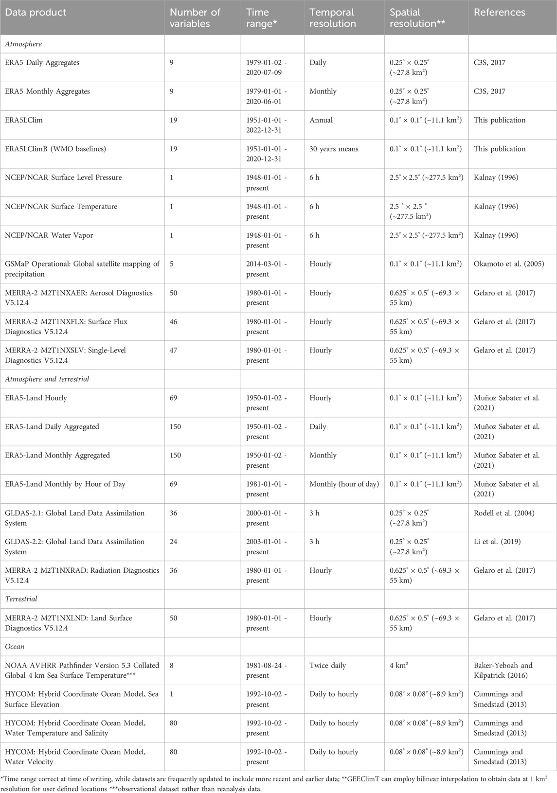
TABLE 1. Description of data products that are currently available in GEEClimT. New datasets can be easily added only if they are available within the Google Earth Engine Data Catalog or within a Google Cloud data bucket that is compatible with Google Earth Engine.

GEEClimT has also been constructed in a manner that allows new datasets to be added as they become available. However, users should note that only data products that exist within the GEE Data Catalog or within Google Cloud data buckets can currently be added to GEEClimT. Requests to add data products to GEEClimT that currently exist in the GEE Data Catalog can be directed to the authors, though requests to add data products that do not currently exist in the GEE Data Catalog should be directed to Google.

1.1.1 ERA5-Land-Climatic (ERALClim) data

GEEClimT also provides access to our new ERA5-Land-Climatic (ERALClim) dataset, providing data for 19 variables (Table 2) at annual resolution (for 1951–2022), and for World Meteorological Organisation (WMO) climate baseline periods (1951-1980; 1961-1990; 1971-2000; 1981-2010; and 1991–2020). These variables are equivalent to the bioclimatic variables of WorldClim (Fick and Hijmans, 2017), though have potentially much broader applications within the environmental and social sciences beyond ecological and biological data where they are traditionally applied. To maintain consistency with WorldClim, the naming of variables is kept the same (i.e., retaining the bio prefix), so that pre-existing workflows that use WorldClim data can be easily adapted to use ERALClim data.

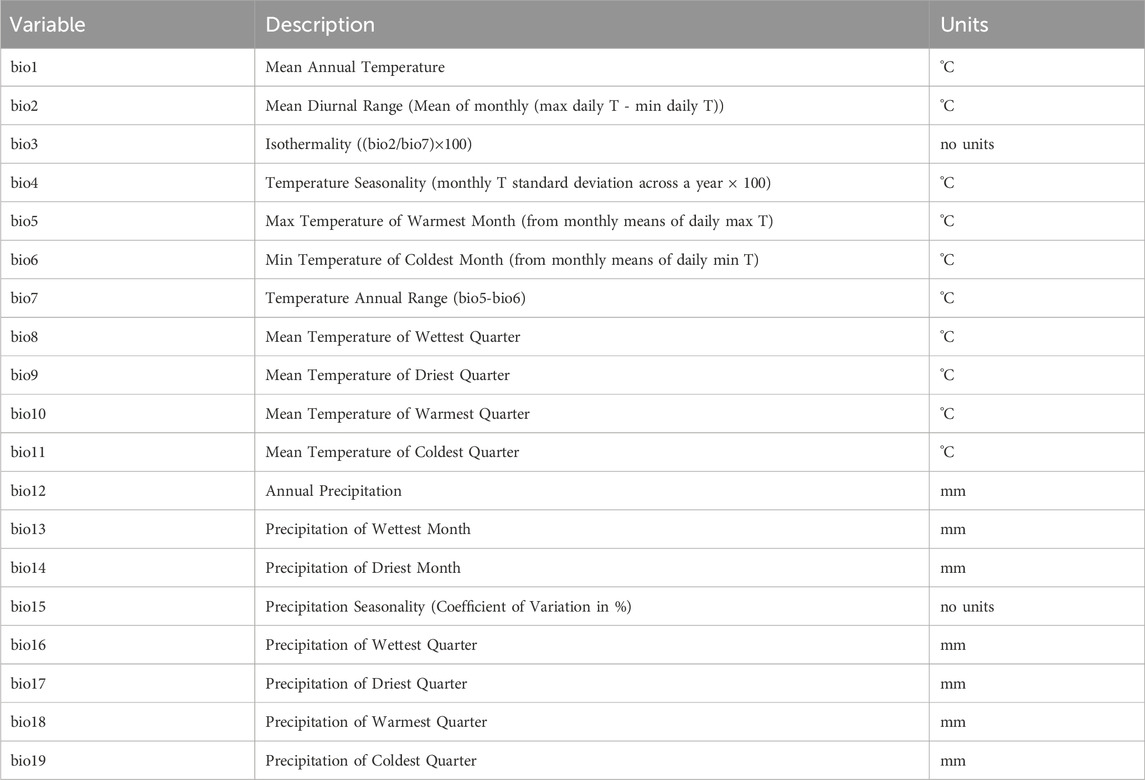
TABLE 2. List of ERALClim variables, description, and units. These variables are comparable to those of WorldClim.

The ERA5-Land Daily Aggregated and Monthly Aggregated data products (Muñoz-Sabater et al., 2021) were used to calculate ERALClim within GEE, and the baseline data are calculated as the average of the resulting annual ERALClim data (access to the annual and baseline datasets are provided through: GEEClimT; GEE; and can also be downloaded as GeoTIFFs outside of GEEClimT as annual data (https://doi.org/10.5281/zenodo.8120646) and climate baseline data (https://doi.org/10.5281/zenodo.8124385)).

The ERALClim data are provided at a spatial resolution of 0.1 × 0.1° (∼11.1 km²), which is equivalent to the spatial resolution of the ERA5-Land reanalysis model inputs. While it would be possible to provide ERALClim data at a finer scale through simply changing the posting level of the output, this is intentionally not done so as to: 1) preserve the original model resolution that the data have been calculated at; and 2) avoid giving users a potentially false impression of the data product’s spatial resolution. Comparisons of ERALClim to WorldClim data for the WorldClim baseline period (1970–2000) where the latter have been regridded from 1 km² to 0.1 × 0.1° spatial resolution are provided in Supplementary Material S1. GEEClimT does optionally provide functionality to obtain data at sub-grid resolution through bilinear interpolation of data to 1 km², but will otherwise return values from the nearest grid point (see below).

Differences between ERALClim and WorldClim are most likely to occur in regions where there is a low spatial or temporal density of meteorological observations. The reason for this is that WorldClim produces spatially continuous data fields through interpolation of observations, while the ERA5-Land data (on which ERALClim are based) physically models conditions based upon a combination of meteorological observations that have been assimilated into the model and the model’s climate physics (Muñoz-Sabater et al., 2021). This in itself does not suggest that one dataset is better than the other in all cases, but highlights that differences between each dataset will arise due to the different methodologies used in the processing of the underlying data.

1.1.2 Using GEEClimT

The following represents a brief description of how to use GEEClimT and its functionality, though a full walkthrough of how to use the tool is provided at the following https://github.com/jmlea16/GEEClimT. A graphical representation of the tool’s workflow is shown in Figure 1.

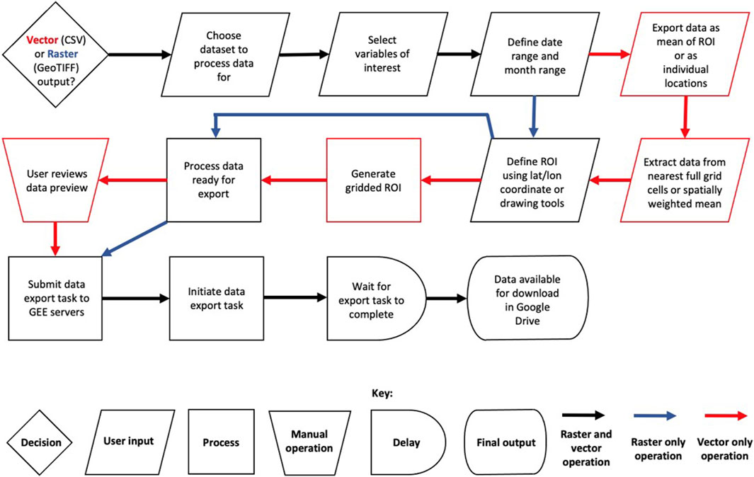
FIGURE 1. GEEClimT workflow diagram.

Users can access a link to the latest version of GEEClimT at the GitHub link above, and access the tool after signing up for a GEE account. No software download is required, and the tool runs entirely in a user’s internet connected browser. Once the GUI has loaded, users can minimise the code editor section of the page that contains GEEClimT’s underlying code. To use GEEClimT users can take the following steps:

1) Select whether data should be output as a CSV or GeoTIFF.

2) Select a reanalysis data product to be queried. GEEClimT will automatically update the temporal range of data that is available in the date text boxes and display a sample data map representing the first time slice that is available for that data product.

3) Select the variables of interest contained within the data product.

4) If needed, edit the date range boxes (strictly in YYYY-MM-DD format) and month range drop down menus to temporally limit the data to be queried.

Where data will be output in CSV format:

5) Select how GEEClimT should handle the data when generating output, either as: a) a single time series representing the mean values of all points that overlap with a user’s region of interest (ROI); or b) multiple time series representing the full record of each grid cell that overlaps with the ROI.

6) Select whether GEEClimT provides output data representing either: a) results from the closest grid cell; or b) use bilinear interpolation to provide data representative of a given location (for a point ROI) or fraction of a grid cell (for a polygon ROI) at 1 km² resolution.

7) Define up to 50 points or one polygon area of interest, by either: a) manually drawing points or a polygon representing regions of interest directly onto the map; or b) defining point locations or a single polygon from comma separated lists of latitude and longitude coordinates expressed in decimal degrees (WGS84 ellipsoid; EPSG: 4,326 projection).

8) Create the gridded ROI, which will show the areas where GEEClimT will extract data for on the map.

9) Extract data using the options and ROI defined previously. The time this will take will depend on the area or number of data points that have been queried. This normally takes a few seconds, though for large datasets may take several minutes. Once data extraction has completed, a new panel will appear on the screen with a preview of the first 1,000 observations (note that if the query contains >1,000 observations, these data have been extracted but are not shown).

10) Initiate export task for all variables selected and all sites queried. Output data are formatted with each column representing a different variable, and each row representing a date and time for a given location/grid cell. To facilitate easy data processing, the central latitude and longitude of each data point is also appended as a data column along with a site name unique to each site.

Reanalysis data in CSV format can therefore be extracted for: individual point locations; all grid point observations that fall within a polygon; mean values across multiple points; or the mean of all grid point observations that fall within a polygon.

If data are to be exported in GeoTIFF format:

1. Define a single polygon (at least three vertices) by importing a list of comma separated latitude and longitude coordinates and clicking the “import polygon” button, or by manually defining a polygon using the drawing tools in the top left corner of the map.

2. Clicking the “Create Export Task” button that will generate export tasks that can be viewed in the “Tasks” tab next to the code editor.

3. Clicking the blue “Run” button for each new export task. For GeoTIFF data, two export tasks are created containing 1) a multilayer GeoTIFF file containing the gridded data; and 2) a CSV file with metadata corresponding to each GeoTIFF layer to aid in post-processing. Note that if the export task contains more than 5,000 layers then GEEClimT will split the request into multiple export tasks.

Exported CSV or GeoTIFF data can be accessed for download to a user’s local machine via the Google Drive account that is associated with their Google Earth Engine account.

1.2 GEECE - CMIP6 climate projection data

Climate projection data provide global, spatially and temporally continuous model output for historical and different potential shared socioeconomic pathway (SSP) scenarios. The sixth Coupled Model Intercomparison Project (CMIP6; Thrasher et al., 2012) undertaken for the sixth Intergovernmental Panel on Climate Change (IPCC) Assessment Report (2021) provide results from multiple climate models projecting future climate for different SSPs. The GEE Data Catalog currently allows access to the results of 34 different model simulations for historical, SSP2-4.5, and SSP5-8.5 scenarios, representing simulations of recent past climate (1950–2015), and future climates (2015–2100) under middling and high emission scenarios respectively.

Data for each scenario are posted at 0.25° spatial resolution and daily temporal resolution, with the majority of simulations providing output for nine variables. A list of these variables and notes on their availability within different simulations are provided in Table 3. Users should note that daily, minimum and maximum temperatures are provided in degrees Kelvin, meaning that conversion to degrees Celsius requires 273.15 to be subtracted from results. Precipitation is also provided as a daily rate with units of kg m⁻² s⁻¹, meaning that daily precipitation totals in millimetres can be obtained by multiplying results by the number of seconds in a day (86,400). Similarly, if data are output at monthly or annual resolution, precipitation values can be converted to monthly or annual totals by multiplying by the number of seconds in the given time unit. Special care should be taken when analysing datasets that are aggregated over specific time intervals, and users should note the units that data are provided in before any conversion is attempted. This information is available through links given in the GEECE interface.

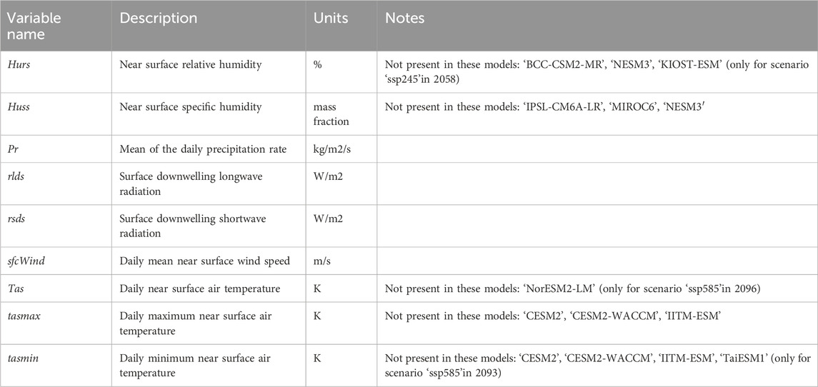
TABLE 3. List and description of variables available for CMIP6 simulations within GEECE.

Users should also note that monthly increments are given in calendar months (i.e. 28 days in February (29 in leap years); 30 days for April, June, September and November; and 31 days for January, March, July, August, October, November and December) rather than equal length months. For annual resolution output, leap years will also be made up of data for 366 days, with non-leap years made up of data for 365 days. Users should also check information within the GEE Data Catalog for how model simulations that have been run to provide 360 days of output per year (‘HadGEM3-GC31-LL’, ‘HadGEM3-GC31-MM’, ‘KACE-1-0-G′, and ‘UKESM1-0-LL’) or 364 days of output per year (‘IITM-ESM’) deal with providing output at 365 or 366 days per year.

GEECE follows a similar workflow to GEEClimT, and while much of the underlying code for the tools is shared, different processing pathways necessitate two separate tools. A full walkthrough of how to use the tool is provided at the following https://github.com/jmlea16/GEECE. A graphical representation of the GEECE’s workflow is shown in Figure 2.

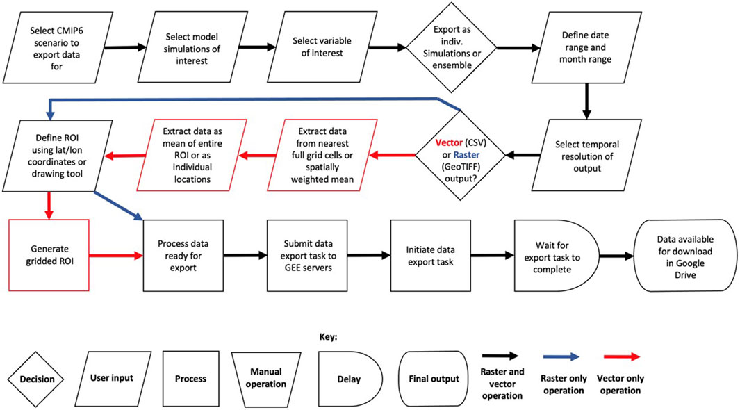
FIGURE 2. GEECE workflow diagram.

GEECE also provides users with options to extract data in CSV or GeoTIFF format, though also allows users to create their own custom simulation ensembles (optionally with their associated standard deviation). When selecting simulations to include in ensembles, it should be noted that some CMIP6 simulations are considered to perform better than others for different variables and geographic regions. Consequently, users may wish to first undertake evaluations of the performance of individual ensemble members before deciding on its final make-up.

Point and raster data for individual simulations or ensembles can be obtained from GEECE by taking the following steps:

1. Select whether output should be from historical, SSP2-4.5 or SSP5-8.5 scenarios

2. Select the simulations to generate output for. Note that the simulations highlighted in blue text in the user interface do not contain output for all variables listed in Table 3. Users should therefore check whether the desired variable(s) to be output are included in the model simulation(s) selected before running the tool. Failure to do so may result in the tool failing to provide output.

3. Select the variables that output should be provided for.

4. Select whether output should be provided for: 1) every simulation selected individually; 2) an ensemble mean of all simulations selected; or 3) an ensemble mean of all simulations selected and the associated ensemble standard deviation.

5. If needed, edit the date range boxes (strictly in YYYY-MM-DD format) and month range drop down menus to temporally limit the data to be queried.

6. Select the timestep of the output either as: 1) daily; 2) monthly; 3) annual; or 4) the mean of the time period selected.

7. Select whether data should be output in CSV or GeoTIFF format.

For outputting in CSV format:

8. Define up to 50 points or one polygon area of interest, by either: a) manually drawing points or a polygon representing regions of interest directly onto the map; or b) defining point locations or a single polygon from comma separated lists of latitude and longitude coordinates expressed in decimal degrees (WGS84 ellipsoid; EPSG: 4,326 projection).

9. Create the gridded ROI, which will show the areas where GEEClimT will extract data for on the map.

10. Extract data using the options and ROI defined previously.

For outputting in GeoTIFF format:

8. Define a single polygon (at least three vertices) by importing a list of comma separated latitude and longitude coordinates and clicking the “import polygon” button, or by manually defining a polygon using the drawing tools in the top left corner of the map.

9. Clicking the “Create Export Task” button that will generate export tasks that can be viewed in the “Tasks” tab next to the code editor.

1.3 Performance of GEEClimT and GEECE

The time that it takes for GEEClimT and GEECE to process, extract and export data will be a function of the volume of data that need to be processed and extracted. Consequently, for a given time period of interest, exporting data from an hourly resolution data product will likely take longer than exporting data for the same time period for a monthly resolution data product. Similarly, exporting data from multiple locations or a region will take longer than for a single point location.

The time that the tools take to execute tasks will also be impacted by how busy the GEE servers are at any given time, and which servers a task is allocated to. GEE users have no control over these aspects when they run any operation within the API, making it challenging to define an expected execution time for any given task. However, GEE does provide an indication of the amount of computational power required to complete each export task in the form of Earth Engine Compute Unit-seconds (EECU-s). While EECU-s do not translate to CPU-seconds due to the way in which the GEE server service is provided, they give an indication of the amount of processing power required to perform each export task.

1.4 Example applications of GEEClimT and GEECE

The following show some simple applications of how data extracted from GEEClimT and GEECE can be used, and aim to highlight some aspects of working with reanalysis data that may be useful for new users. These examples are by no means comprehensive in terms of potential applications or issues that users may encounter, and focus primarily on how data extracted from the tools can facilitate easy analysis in environmental and ecological applications.

1.4.1 Case study 1: comparing observations, reanalysis data, and future climate projections in Greenland

Within glaciology reanalysis and projection data have significant potential for informing investigations into the past, present and future of the Greenland Ice Sheet (GrIS). The low density of meteorological stations across the ice sheet and significant climate gradients from non-glaciated coastal regions to the ice sheet interior mean that observations at one location can differ substantially from conditions experienced a short distance (<10 s km) away. Reanalysis and projection data that are generated by physically based climate models can therefore provide data that are likely to be more representative of a particular locality where weather station data are unavailable. However, reanalysis data can also be subject to spatially varying biases related to the underlying model physics and density of observations (e.g., Cucchi et al., 2020), while the spatial resolution over which both reanalysis and projections are conducted is frequently incapable of resolving local topographic effects and sub-grid resolution weather variability.

In this example, we highlight these effects by comparing ERA5-Land data for Greenland’s capital city Nuuk (64.2000⁰ N 51.6833⁰ W; Jensen et al., 2022), and the on-ice PROMICE weather station KAN_U (67.0007⁰ N 47.0243⁰ W; Fausto et al., 2021; How et al., 2022). These sites are chosen given that Nuuk is a coastal city with significant surrounding topography that is also frequently affected by local conditions off-shore (e.g., sea fog), while KAN_U is located toward the ice sheet interior with little topographic variability and is influenced by general synoptic conditions. Both Nuuk and KAN_U weather stations provide data at hourly resolution, with the analysis below using all data where corresponding ERA5-Land reanalysis data were available (1 November 2000 to 31 December 2021; and 4 April 2009 to 27 March 2023 respectively). It should be noted that while ERA5-Land atmospheric data variables have higher spatial resolution than ERA5 data, these represent lapse-rate corrected regridding of ERA5 data (Muñoz Sabater et al., 2019; https://cds.climate.copernicus.eu/cdsapp#!/dataset/10.24381/cds. e2161bac?tab=overview; accessed: 26/6/2023).

Comparison of observations to reanalysis data were performed at hourly, daily and monthly temporal resolution, with an ensemble of 24 CMIP6 models used to obtain data for historical (1950–2015), and SSP2-4.5 and SSP5-8.5 projection scenarios (2015–2,100) at annual resolution (Figure 3; Bentsen et al., 2019; Byun et al., 2019; Dix et al., 2019; EC-Earth Consortium, 2019a; EC-Earth Consortium, 2019a; Guo et al., 2018; Hajima et al., 2019; Jungclaus et al., 2019; Krasting et al., 2018; Li, 2019; Lovato et al., 2021; Lovato and Peano, 2020; NASA Goddard Institute for Space Studies, 2018; Ridley et al., 2018; Ridley et al., 2019; Volodin et al., 2019a; 2019b; Wieners et al., 2019; Yukimoto et al., 2019; Ziehn et al., 2019). The CMIP6 ensemble excludes simulations available in GEECE where there are any missing data (Boucher et al., 2018; Tatebe and Wanatabe, 2018; Xin et al., 2018; Danabasoglu, 2019a; Danabasoglu, 2019b; Cao and Wang, 2019; Kim et al., 2019; Lee and Liang, 2019; Panickal et al., 2019; Seland et al., 2019).

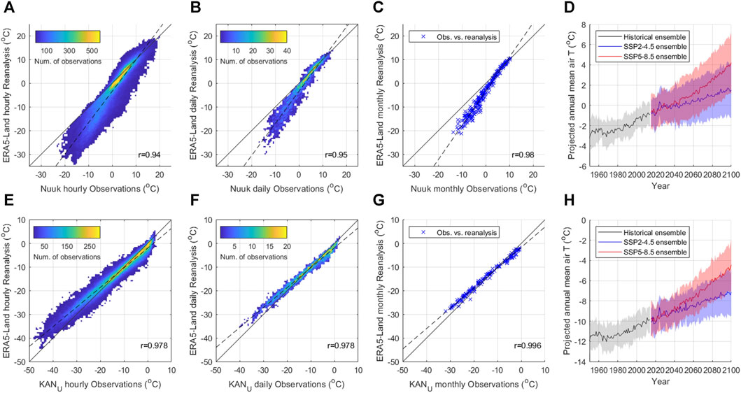
FIGURE 3. Results of 2 m air temperature weather station observations compared to ERA5-Land reanalysis data products for Nuuk (A–C), and KAN_U (E–G) obtained from GEEClimT. Results showing the annual mean and standard deviation of a 24 member ensemble of CMIP6 model simulations for historical, SSP2-4.5 and SSP5-8.5 scenarios processed using GEECE are also shown for Nuuk (D) and KAN_U (H). Note that panels (A, B, E, F) show the density of data points within 0.5°C intervals.

To enable comparison with observations, ERA5-Land 2 m air temperature data (Muñoz-Sabater et al., 2021) were extracted using GEEClimT from Hourly, Daily Aggregated and Monthly Aggregated data products, while GEECE was used to define the CMIP6 model ensemble, process input data from daily to annual resolution, and calculate respective ensemble means and standard deviations for the time series. Within the tools we take advantage of GEEClimT and GEECE’s functionality for extracting to a CSV file data from given point locations where values are interpolated from the nearest four grid cells, though users should note the different spatial resolutions of the climate projection data (0.25 × 0.25°) and ERA5-Land reanalysis data (0.1 × 0.1°). Through using the point interpolation option in the tools we aim to mitigate the effects of the topography around Nuuk, though the differing spatial resolutions of the underlying data place limits on direct comparison. Observational data for each site were resampled to the corresponding ERA5-Land data product time interval by taking the mean of available observations. Time periods where observation data were missing within each timestep were discarded from the analysis.

Results show strong correlations exist at all temporal intervals between observations and ERA5-Land reanalysis data products for both Nuuk and KAN_U locations. However, ERA5-Land data for Nuuk show evidence for a cold bias that increases with more negative temperatures. This bias is replicated at hourly, daily and monthly temporal intervals, though the correlation between observations and reanalysis is observed to strengthen with longer temporal intervals (Figures 3A–C). At KAN_U, less bias is observed between reanalysis and observational data compared to Nuuk, though ERA5-Land data do exhibit a warm bias at the coldest temperatures (Figures 3E–G). Stronger correlations between observations and ERA5-Land data are found at KAN_U than at Nuuk for all temporal intervals analysed. Results from the CMIP6 ensemble show that Nuuk and KAN_U are projected to experience similar magnitudes of warming for SSP2-4.5 and SSP5-8.5 by 2,100, with divergence between the two projection scenarios beginning in approximately 2040 for both locations (Figures 3D, H).

Differences in the strength and bias of relationships observed at Nuuk and KAN_U likely reflect a combination of inherent model bias, regridding effects associated with ERA5-Land using downscaled data from ERA5 output, the inability of the reanalysis model to resolve the effects of sub-grid topographic variability (i.e., high variability at Nuuk resulting in weaker correlations compared to low variability at KAN_U), and sub-grid scale variability in weather conditions (also higher at Nuuk than at KAN_U). The warm bias of reanalysis data at KAN_U at lower temperatures may also be partly explained by winter snow accumulation partially burying the weather station, effectively raising the land surface meaning that the temperature sensor height may be < 2 m.

The above example aims to highlight that while reanalysis data will likely be strongly correlated to reality, biases may exist; outliers become more likely at shorter time intervals; sub-grid scale topography and local weather variability will impact the accuracy of reanalysis data; and how the observational data have been acquired all need to be considered before taking results of reanalysis data at face value.

1.4.2 Case study 2: species distribution modelling - red eyed damselfly (Erythromma najas)

A key approach within biology, ecology and evolution is to correlate biological data with the abiotic environment (e.g., climate, topography) to establish mechanistic links between the environment and species distributions, with this approach broadly being referred to as biogeography (Lomolino et al., 2017). Such biogeography studies can be used to inform on population characteristics, demography, species distributions, biodiversity and responses to climate change (Fitt and Lancaster, 2017; Lomolino et al., 2017). The ability to access high quality, geolocated abiotic environmental data therefore holds huge importance. Here, we demonstrate the utility of GEEClimT for such studies, demonstrating its application in species distribution modelling (SDM) of a native British damselfly, Erythromma najas.

Within this case study, results from SDM’s will be compared between models where climate variables were obtained from ERALClim dataset within GEEClimT, and models where WorldClim V2 (Fick and Hijmans, 2017) environmental variables were used. In this case study GEEClimT is used to extract a raster grid of ERALClim data of the British Isles from a user drawn polygon and download equivalent WorldClim V2 data that are both clipped to the United Kingdom borders in post processing. WorldClim V2 represents the environmental dataset most widely used for this application (Title and Bemmels, 2018), while ERALClim represents a new dataset developed in this study that is comparable to WorldClim, derived from ERA5-Land data (Munoz-Sabater et al., 2021).

Bioclimatic variables were assessed for co-linearity, and variables with a correlation score greater than 0.8 were removed, leaving Bio1, 2, 3, 4, 5, 8, 9, 10, 15, and 18. For ERALClim and WorldClim inputs, species distributions were modelled using maximum entropy habitat suitability model implemented in MaxEnt, version 3.4.3 (Phillips et al., 2006) using the Dismo package for R (Hijmans et al., 2019). Species’ presence points were downloaded from the Global Biodiversity Information Facility (http://www.gbif.org; https://doi.org/10.15468/dl.hdeere), with duplicate records and records which did not fall within both a ERALClim and WorldClim raster cell being removed, leaving 9,485 presence points (Figure 4A).

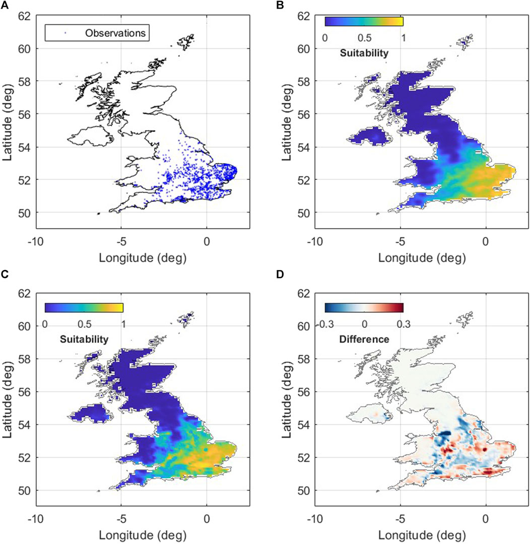
FIGURE 4. Plots showing (A) location of observations of Erythromma najas (n = 9,485) across the United Kingdom used as input for (B) species distribution model constrained by ERALClim data, and (C) species distribution model constrained by WorldClim v2 data. The difference in suitability scores between ERALClim and WorldClim v2 species distribution models is shown in panel (D) where positive values indicate higher suitability scores for ERALClim and negative values indicate higher suitability scores for WorldClim.

The MaxEnt models were run five times using default parameters, withholding a separate 20% of presence points for model testing on each model run. The final niche model for each species represented the average habitat suitability calculated across the five model runs. Model fit was also assessed by estimating the area under the Receiver Operating Characteristic (ROC) curve (AUC), with both models having an AUC greater than 0.8.

Results highlight limited agreement in model results between the WorldClim and ERALClim datasets, where Bio10 has the both the highest contribution and permutation importance when the data is modelled with ERALClim data, while Bio5 is the most important and has highest contribution when modelled with WorldClim (Table 4). Likewise, when comparing suitability maps, while there is general agreement in the projected suitability (Figures 4B, C), there are distinct differences (Figure 4D). These differences within this case study, can have profound impact of the interpretation of results, given that SDM’s are often used to inform conservation decision making, such as species reintroduction (Barlow et al., 2021), or making predictions of range shifts under climate change (Jarvie and Svenning, 2018).

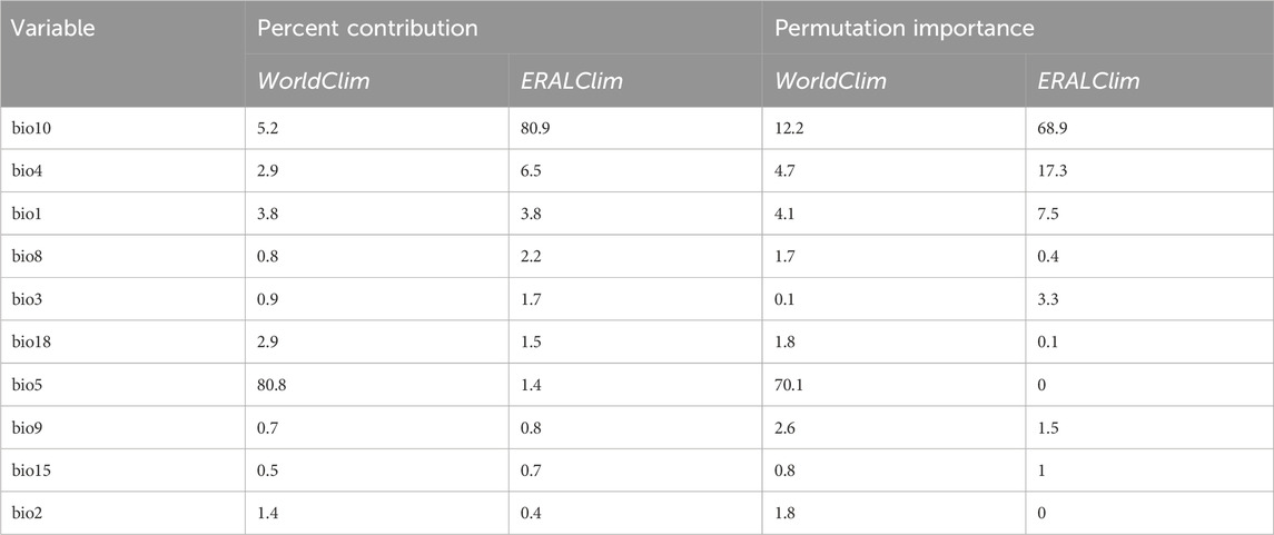
TABLE 4. Percentage contribution and permutation importance for species distribution models that are constrained by WorldClim and ERALClim for Erythromma najas.

While this case study does not have the power to suggest that one dataset performs better than another, results here do highlight the importance of climate dataset choice when conducting biogeographical studies. As demonstrated here, results can vary significantly, and can have meaningful impact on the interpretation of results. It is therefore important to have access to a wide range of environmental data to enable accurate studies of the relationship between the environment and biological systems.

1.4.3 Case study 3: estimating crop yields - miscanthus

Within the disciplines of Biology, Ecology and Evolution, it is commonplace to correlate biological data with abiotic environmental data so that mechanistic links and genotype by environment associations can be derived. Here, we demonstrate with a simple example the utility of this dataset for applications in ecological and biological studies. Miscanthus is a perennial C4 grass that is used as a biofuel primarily for combustion and occasionally for anaerobic digestion, with approx. 20,000 ha commercially grown in the EU and some 8,286 ha grown in the United Kingdom (EU CORDIS, 2016; DEFRA, 2021).

Originating from Asia, Miscanthus has now been bred to produce a range of varieties that are more suitable for European and United Kingdom climates (Clifton-Brown et al., 2004; Heaton et al., 2010; Brown et al., 2013). Within the United Kingdom, yields of Miscanthus can vary markedly as a result of several environmental factors, of which, temperature is a key abiotic driver of yield (Purdy et al., 2013; Awty-Carroll et al., 2023). Using ERA5-Land data obtained from GEEClimT we have correlated Miscanthus yields across 8 sites within the United Kingdom. All available yield data that was geolocated were included, providing 44 data points from 8 sites. Using the same interpolation approach employed in case study 1 the latitude and longitude were extracted from these points and placed into GEEClimT, extracting all data available from the ERA5-Land data product for the period 1990 and 2022. These data were downloaded as a. csv file, and read into R v 4.2.2 for further analysis (R Core Team, 2021).

The data for mean annual soil temperature and for mean volumetric soil water (MVSW), was selected to investigate these key abiotic drivers in relation to Miscanthus harvestable yield. For each site, the average was calculated for the period spanning when the Miscanthus rhizomes were planted to when they were harvested, and for the 12 months preceding harvest. Correlations were then obtained between yield and the abiotic environmental data sets calculated using linear models. Results demonstrated that yield decreased with increasing mean soil temperature, in the 12 months preceding harvest (Effect = 66.88 ± 16.48, df = 39.52, t = 4.06, p < 0.001, Figure 5B). Conversely, yield increased with increasing MVSW (Effect = −2.14 ± 0.87, df = 38.47, t = −2.45, p = 0.019, Figure 5A). This aligns with our understanding that Miscanthus is adapted to a cool and moist climate (Beale et al., 1996; Purdy et al., 2013).

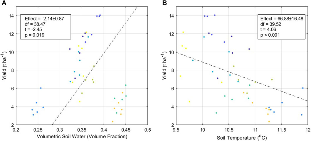
FIGURE 5. Results of linear modelling of (A) volumetric soil moisture values obtained from ERA5-Land data using GEEClimT versus Miscanthus yield per hectare; and (B) soil temperature values obtained from ERA5-Land data using GEEClimT versus Miscanthus yield per hectare. Colour of points indicate different site locations.

This analysis acts as a working example of how climate derived data from GEEClimT can be used to forecast yields and could be utilised as a tool for identifying suitable locations for Miscanthus crop production, or optimal locations for other crop species. At a local level, farmers and growers can increase their localised species-specific productivity by identifying species that are best adapted within their local environmental mosaic. Not only does this highlight the suitability for reanalysis climate data to be used to biological studies but illustrates the potential accessibility that GEEClimT allows for ease of access, opening up a wider range of data to biologists without the need for technical knowledge or specialist software skills.

1.4.4 Case study 4: comparison of NCEP/NCAR reanalysis data with ERA5-Land along a latitudinal gradient

Multiple reanalysis products provide data output that represent similar variables. However, for each data product, results will likely differ depending on (amongst other factors): the underlying physics of the model used to generate the output; the observations used to drive the model; the data assimilation schemes used to incorporate data into the model; and the spatial resolution that the simulations are conducted at. In this example, we compare results of 2 m air temperature output from the 2.5⁰ resolution NCEP/NCAR Reanalysis dataset (Kalnay, 1996), and the 0.1⁰ resolution ERA5-Land Monthly Aggregated dataset (Muñoz-Sabater et al., 2021) for the period 1951-2022 at annual temporal resolution. To illustrate how these results can vary along a latitudinal gradient, data were extracted using GEEClimT for every 10th degree of latitude from 80⁰S to 80⁰N along the 20⁰W line of longitude by directly defining latitude and longitude within the tool. This line of longitude was chosen to maximise data availability for the ERA5-Land dataset, given that it does not provide output over oceans. NCEP/NCAR Reanalysis Data are provided at 6 hourly intervals, while we take advantage of the ERA5-Land Monthly Aggregated product to minimise GEEClimT processing and post-processing times. For this scenario, GEEClimT took approximately 3 h to extract the NCEP/NCAR data (providing data for 17 locations, and a total of 1,874,760 data values), and less than 1 minute to extract the ERA5-Land data (providing data for 10 locations, and a total of 8,800 data values). Output data were subsequently imported into MatlabⓇ and to allow calculation of annual means for each latitude for each reanalysis product.

Results from both reanalysis products capture expected temperature variability with latitude (Figures 6A, C), and display late 20th century/early 21st century warming trends (Figures 6B, D). However, differences between the data products are observed in both the absolute temperatures provided for each location (Figure 6C) and in the magnitude of the temperature anomalies compared to the 1961–1990 mean baseline temperatures (Figures 6D–F).

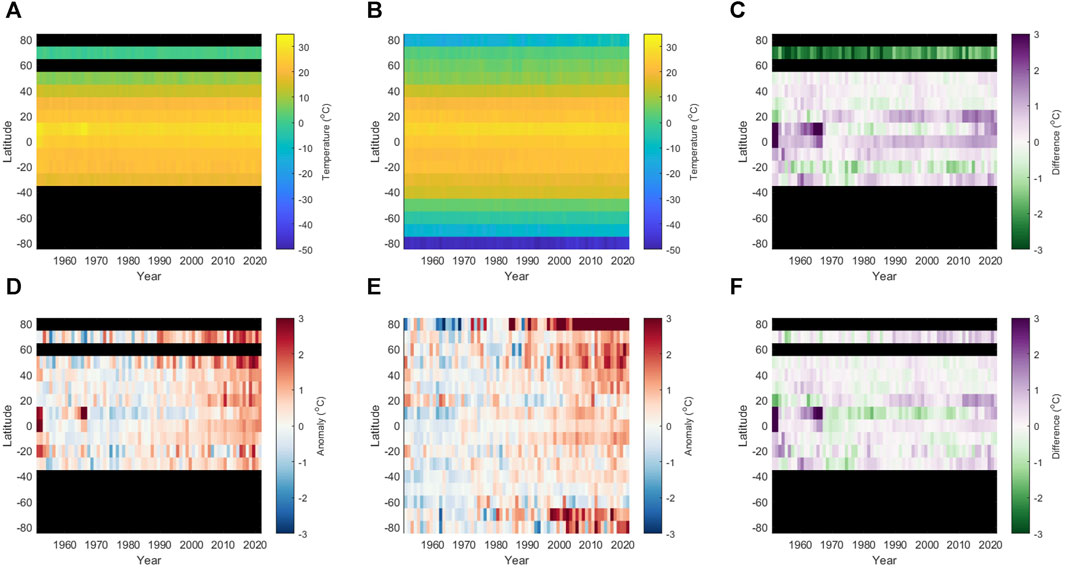
FIGURE 6. Annual mean 2 m air temperature data output for ERA5-Land and NCEP/NCAR Reanalysis data products for 1951–2022 by latitude along 20⁰W line of longitude, showing: (A) absolute temperatures obtained from ERA5-Land, and (B) from NCEP/NCAR Reanalysis; (C) the difference between ERA5-Land and NCEP/NCAR; (D) the 2 m air temperature anomaly for ERA5-Land data using a baseline mean value from 1961 to 1990 calculated for each latitude; (E) as (D) but for NCEP/NCAR Reanalysis data; and (F) the difference in 2 m air temperature anomalies between ERA5-Land and NCEP/NCAR Reanalysis. All locations where no data are available or no comparison was possible are shown in black.

In addition to previously mentioned influences on the values provided by reanalysis data, at least part of the differences observed between these two datasets can be accounted for due to the differing spatial resolutions of the reanalysis output, and the manner in which GEEClimT extracts data from them (i.e., using bilinear interpolation of the nearest grid cells to obtain values for a given location). GEEClimT output from coarser spatial resolution data (e.g., NCEP/NCAR) will therefore be influenced by grid values that cover larger areas than finer resolution datasets (e.g., ERA5-Land). It is also worth reiterating at this point that ERA5-Land output at 0.1⁰ resolution is equivalent to lapse-rate corrected data from ERA5 simulations performed at 0.25⁰ resolution.

1.4.5 Case study 5 - identifying periods of drought and flood risk using standardised precipitation index (SPI)

Hydrological extremes such as floods and droughts are major climate related hazards with methods that allow estimations of their probability of occurrence and magnitude being of much use. One such measure is the Standardised Precipitation index (SPI) (Mckee et al., 1993), one of the World Meteorological Organisation’s key drought indexes used in drought prediction and assessment.

The SPI requires only precipitation as an input data source which can be useful in data sparse environments. Use of reanalysis data (that provide data averaged over a grid cell or region), can be a useful addition to this in providing an indication of conditions over an area, rather than just at an individual point. The SPI is based on the probability of precipitation within a chosen time interval and is outputted as a monthly value. This is achieved through first fitting precipitation input data to a gamma distribution that are then transformed to a normal distribution. SPI values are computed over running time intervals (Mckee et al., 1993), with traditional intervals of 3, 6, and 12–48-month timescales being representative of meteorological, ecological, and longer-term hydrological drought (affecting groundwater and reservoir reserves) respectively. The monthly SPI value calculated represents the deviation from the recent long-term mean (i.e., the time interval), with negative numbers representing relatively dry periods and positive relatively wet periods–the more extreme the value, the more extreme the period. In addition to drought, the ability to identify periods of extreme precipitation provides a means to assess the meteorological conditions preceding flooding.

Here, we provide examples of the use of both GEEClimT and GEECE to obtain precipitation data (from ERA5 (Muñoz Sabater et al., 2019) and a 24 model CMIP ensemble respectively) in the investigation of recent hydrometeorological extremes and investigate the potential impacts of climate change on droughts in areas previously determined to be at risk. CSV files of data for each location were obtained through copy and pasting the polygon coordinates of each area of interest directly into GEEClimT and GEECE.

First, we focussed on the California (United States) drought of 2012–2016, focussing on El Dorado Forest where drought conditions were so severe tree mortality reached almost 50% (Fettig et al., 2019). SPI was computed for a 12-month interval (SPI-12) representing hydrological drought from 1980–2021 (Figure 7A). In this example SPI clearly identifies the 2012 to 2016 drought as the most intense (most negative SPI) of the study period, second only to the drought in the early 2000s.

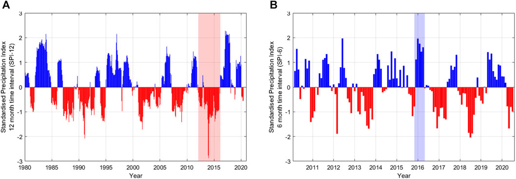
FIGURE 7. SPI indices for (A) 1980 - 2021 for a 12-month interval (SPI-12) for El Dorado Forest in CA, United States, with drought period mentioned in the text highlighted by red shading; and (B) a 6-month interval (SPI-6) for Aberdeenshire, United Kingdom, with wet period mentioned in the text highlighted by blue shading.

ERA5 Monthly Aggregated precipitation data extracted from GEEClimT was then used to investigate a wetter period for a different location, with the late December 2015–January 2016 floods in Aberdeenshire, Scotland chosen (Figure 7B). For this example, an interval of 6 months was chosen (SPI-6) as it represents soil water stores, and the flooding was linked to an ongoing wet period and lack of soil water storage capacity (Soulsby et al., 2017). Here while the late December 2015–January 2016 wet period is clearly visible; it was not the most intense event (second to March-July 2012). The SPI index does however clearly show the large magnitude of the wet period, as all bars between December 2015 to April 2016 exceed an SPI of +1.

Finally, we applied the SPI technique to CMIP6 ensemble data obtained via GEECE. ERA5-Land, CMIP6 historical scenario data, SSP2-4.5 and SSP5-8.5 data were downloaded for Dorset, United Kingdom, which has been identified as being susceptible to drought with projected changes in climate (Arnell et al., 2021). A mean of the 24 member model ensemble was used at a monthly time step to calculate SPI over a 24-month interval (SPI-24), representative of long-term hydrological drought. The historical period (defined here as 1955–2005), and future projections using SSP2-4.5 (medium emissions) and SSP5-8.5 (high emissions) scenarios for 2020-2050 were then compared to identify changes in drought duration (months of negative SPI), magnitude (sum of all SPIs within the drought), and intensity (maximum SPI during drought) (Table 5)).

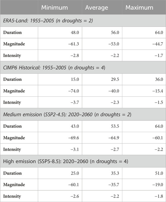
TABLE 5. Comparison of the minimum, average, and maximum values for the duration, magnitude, and intensity of long term (SPI-24) droughts in Dorset between: the 1955–2005 ERA5-Land data, the 1955–2005 historical scenario data, and 2020–2060 projected data for both medium (SSP4.5 and high (SSP8.5) emission scenarios.

While caution should be applied as this analysis only considers precipitation and no other variables associated with other elements of climate change, the analysis suggests that under medium emissions scenarios that the intensity of long-term extreme (<-1.5 intensity) hydrological drought remains similar to the historical period, though there will likely be increases in the duration, intensity and magnitude of these hydrometeorological hazards in the future. Mismatch between the ERA5 and the CMIP6 historical scenario may result from using the ensemble mean values as input for the SPI, which will dampen monthly variability that may be captured by individual simulations. Similar caveats apply to results driven by the SSP2-4.5 and SSP5-8.5 ensemble means, highlighting that users should carefully consider how or if the assumptions made in datasets extracted from GEEClimT and GEECE may impact the results of subsequent analysis.

The data used within this analysis was identified and processed for download in <15 min before being used in the relatively simple SPI analysis. This highlights the use of the tool in accessing data from anywhere on the planet - something traditionally difficult and time consuming–and applying it to real world, beneficial analyses enabling assessment of conditions before, during, and after extreme hydrometeorological events, as well as understanding potential future scenarios.

2 Summary

GEEClimT and GEECE offer the potential to dramatically improve the ease of access to reanalysis and climate projection data, broadening its user base amongst researchers, students and instructors. The tools are free to use for research and educational purposes, though can also be used for commercial applications (strictly only through direct correspondence with the authors).

The new annual resolution ERALClim dataset included within GEEClimT also represents a significant extension of the WorldClim (BioClim) data product, providing global scale bioclimatic variables for 1951-2022 and climate baseline summaries for five different WMO climate baselines from 1951 to present. Derivation of ERALClim from ERA5-Land Hourly data ensures that results provided are based on a combination of climate physics and assimilated observations rather than spatial interpolation of observations alone.

Through the point-and-click interfaces of GEEClimT and GEECE, they provide a single location to access 24 different reanalysis data products, and three climate scenarios for 34 different model simulations respectively. In doing so, GEEClimT and GEECE address multiple existing barriers to accessing these data through: 1) not requiring any coding experience to process and obtain full time series of data from user defined regions of interest; 2) by limiting analysis to a user’s ROI, they remove the requirement to download substantial volumes of potentially superfluous data (compared to where data products can only be downloaded as full global model domains); 3) removing potentially laborious post-processing steps through provision of output data in commonly used spreadsheet or raster data formats (rather than specialist netCDF or GRIB formats); and 4) processing and analysing data in a cloud computing environment, meaning that users are not limited by the processing power or storage capacity of their local machines. The case studies presented of how data obtained through GEEClimT and GEECE can be applied to environmental and biological problems, though illustrate only a small range of its potential applications.

Together, GEEClimT and GEECE therefore provide a means to ensure that the significant potential of reanalysis data across environmental, biological and social sciences can be more easily realised by a wider range of researchers and students across multiple disciplines.

Data availability statement

The datasets presented in this study can be found in online repositories. The names of the repository/repositories and accession number(s) can be found in the article/Supplementary Material.

Author contributions

JL: Conceptualization, Data curation, Formal Analysis, Funding acquisition, Investigation, Methodology, Resources, Software, Supervision, Validation, Visualization, Writing–original draft, Writing–review and editing. RF: Conceptualization, Formal Analysis, Methodology, Validation, Writing–original draft, Writing–review and editing. SB: Formal Analysis, Investigation, Methodology, Supervision, Validation, Writing–original draft, Writing–review and editing. GC: Methodology, Resources, Validation, Writing–original draft, Writing–review and editing. JD: Formal Analysis, Investigation, Methodology, Validation, Writing–original draft, Writing–review and editing. NJ: Methodology, Resources, Validation, Writing–original draft, Writing–review and editing. RW: Formal Analysis, Investigation, Methodology, Validation, Writing–original draft, Writing–review and editing.

Funding

The author(s) declare financial support was received for the research, authorship, and/or publication of this article. JL’s contribution to this work was supported by their UKRI Future Leaders Fellowship (MR/S017232/1 and MR/X02346X/1).

Acknowledgments

We acknowledge the World Climate Research Programme, which, through its Working Group on Coupled Modelling, coordinated and promoted CMIP6. We thank the climate modelling groups for producing and making available their model output, the Earth System Grid Federation (ESGF) for archiving the data, and the multiple funding agencies who support CMIP6 and ESGF. Anonymised Miscanthus yield data used in case study 3 was provided by Terravesta Assured Energy Crops Ltd. The authors wish to acknowledge Prof. Ed Hawkins (University of Reading, United Kingdom) for inspiring the “warming stripes” colour scheme for Figures 6D, E.

Conflict of interest

The authors declare that the research was conducted in the absence of any commercial or financial relationships that could be construed as a potential conflict of interest.

Publisher’s note

All claims expressed in this article are solely those of the authors and do not necessarily represent those of their affiliated organizations, or those of the publisher, the editors and the reviewers. Any product that may be evaluated in this article, or claim that may be made by its manufacturer, is not guaranteed or endorsed by the publisher.

Supplementary material

The Supplementary Material for this article can be found online at: https://www.frontiersin.org/articles/10.3389/fenvs.2024.1294446/full#supplementary-material

Supplementary Presentation 1 | Maps comparing results of each variable of ERALClim averaged for the period 1970–2000 to those of WorldClim.

References

Adeyeye, T. E., Insaf, T. Z., Al-Hamdan, M. Z., Nayak, S. G., Stuart, N., DiRienzo, S., et al. (2019). Estimating policy-relevant health effects of ambient heat exposures using spatially contiguous reanalysis data. Environ. health 18 (1), 35–13. doi:10.1186/s12940-019-0467-5
Arnell, N. W., Kay, A. L., Freeman, A., Rudd, A. C., and Lowe, J. A. (2021). Changing climate risk in the UK: a multi-sectoral analysis using policy-relevant indicators. Clim. Risk Manag. 31, 100265. doi:10.1016/j.crm.2020.100265
Awty-Carroll, D., Magenau, E., Al Hassan, M., Martani, E., Kontek, M., van der Pluijm, P., et al. (2023). Yield performance of 14 novel inter- and intra-species Miscanthus hybrids across Europe. GCB Bioenergy 15 (4), 399–423. doi:10.1111/GCBB.13026
Baker-Yeboah, S., and Kilpatrick, K. A. (2016). Pathfinder version 5.3 AVHRR sea surface temperature climate data record. AGU Fall Meet. Abstr. 2016, OS43A–2005.
Barlow, M. M., Johnson, C. N., McDowell, M. C., Fielding, M. W., Amin, R. J., and Brewster, R. (2021). Species distribution models for conservation: identifying translocation sites for eastern quolls under climate change. Glob. Ecol. Conservation 29, e01735. doi:10.1016/j.gecco.2021.e01735
Beale, C. V., Bint, D. A., and Long, S. P. (1996). Leaf photosynthesis in the C4-grass Miscanthus x giganteus, growing in the cool temperate climate of southern England. J. Exp. Bot. 47 (295), 267–273. doi:10.1093/jxb/47.2.267
Bentsen, M., et al. (2019). NCC NorESM2-MM model output prepared for CMIP6 CMIP. Earth Syst. Grid Fed. doi:10.22033/ESGF/CMIP6.506
Boucher, O., et al. (2018). IPSL IPSL-CM6A-LR model output prepared for CMIP6 CMIP. Earth Syst. Grid Fed. doi:10.22033/ESGF/CMIP6.1534
Brown, J. C., Robson, P., Davey, C., Farrar, K., Hayes, C., Huang, L., et al. (2013). “Breeding Miscanthus for bioenergy,” in Bioenergy feedstocks: breeding and genetics (China: Wiley). doi:10.1002/9781118609477.ch5
Byun, Y.-H., et al. (2019). NIMS-KMA KACE1.0-G model output prepared for CMIP6 CMIP. Earth Syst. Grid Fed. doi:10.22033/ESGF/CMIP6.2241
Cao, J., and Wang, B. (2019). NUIST NESMv3 model output prepared for CMIP6 CMIP. Earth Syst. Grid Fed. doi:10.22033/ESGF/CMIP6.2021
Clifton-Brown, J. C., Stampfl, P. F., and Jones, M. B. (2004). Miscanthus biomass production for energy in Europe and its potential contribution to decreasing fossil fuel carbon emissions. Glob. Change Biol. 10 (4), 509–518. doi:10.1111/j.1529-8817.2003.00749.x
Cucchi, M., Weedon, G. P., Amici, A., Bellouin, N., Lange, S., Müller Schmied, H., et al. (2020). WFDE5: bias-adjusted ERA5 reanalysis data for impact studies. Earth Syst. Sci. Data 12, 2097–2120. doi:10.5194/essd-12-2097-2020
Cummings, J. A., and Smedstad, O. M. (2013). Variational data assimilation for the global ocean. Data assimilation for atmospheric, oceanic and hydrologic applications vol II. Berlin, Heidelberg: Springer, 303–343. chapter 13.
Danabasoglu, G. (2019a). NCAR CESM2 model output prepared for CMIP6 CMIP. Earth Syst. Grid Fed. doi:10.22033/ESGF/CMIP6.2185
Danabasoglu, G. (2019b). NCAR CESM2-WACCM model output prepared for CMIP6 CMIP. Earth Syst. Grid Fed. doi:10.22033/ESGF/CMIP6.10024
DEFRA (2021). Official Statistics: section 2: plant biomass: miscanthus, short rotation coppice and straw. Available at: https://www.gov.uk/government/statistics/area-of-crops-grown-for-bioenergy-in-england-and-the-uk-2008-2020/section-2-plant-biomass-miscanthus-short-rotation-coppice-and-straw.
Dix, M., et al. (2019). CSIRO-ARCCSS ACCESS-CM2 model output prepared for CMIP6 CMIP. Earth Syst. Grid Fed. doi:10.22033/ESGF/CMIP6.2281
EC-Earth Consortium (EC-Earth) (2019a). EC-Earth-Consortium EC-Earth3 model output prepared for CMIP6 CMIP. Earth Syst. Grid Fed. doi:10.22033/ESGF/CMIP6.181
EU CORDIS (2016). Optimizing miscanthus biomass production. Available at: https://cordis.europa.eu/project/id/289159/reporting.
Fausto, R. S., van As, D., Mankoff, K. D., Vandecrux, B., Citterio, M., Ahlstrøm, A. P., et al. (2021). Programme for Monitoring of the Greenland Ice Sheet (PROMICE) automatic weather station data. Earth Syst. Sci. Data 13, 3819–3845. doi:10.5194/essd-13-3819-2021
Fettig, C. J., Mortenson, L. A., Bulaon, B. M., and Foulk, P. B. (2019). Tree mortality following drought in the central and southern Sierra Nevada, California, US. For. Ecol. Manag. 432, 164–178. doi:10.1016/j.foreco.2018.09.006
Fick, S. E., and Hijmans, R. J. (2017). WorldClim 2: new 1-km spatial resolution climate surfaces for global land areas. Int. J. Climatol. 37 (12), 4302–4315. doi:10.1002/joc.5086
Fitt, R. N. L., and Lancaster, L. T. (2017). Range shifting species reduce phylogenetic diversity in high latitude communities via competition. Jounral Animal Ecol. 86 (3), 543–555. doi:10.1111/1365-2656.12655
Gelaro, R., McCarty, W., Suárez, M. J., Todling, R., Molod, A., Takacs, L., et al. (2017). The modern-era retrospective analysis for research and applications, version 2 (MERRA-2). J. Clim. 30 (14), 5419–5454. doi:10.1175/jcli-d-16-0758.1
Gorelick, N., Hancher, M., Dixon, M., Ilyushchenko, S., Thau, D., and Moore, R. (2017). Google Earth engine: planetary-scale geospatial analysis for everyone. Remote Sens. Environ. 202, 18–27. doi:10.1016/j.rse.2017.06.031
Guo, H., et al. (2018). NOAA-GFDL GFDL-CM4 model output. Earth Syst. Grid Fed. doi:10.22033/ESGF/CMIP6.1402
Hajima, T., et al. (2019). MIROC MIROC-ES2L model output prepared for CMIP6 CMIP. Earth Syst. Grid Fed. doi:10.22033/ESGF/CMIP6.902
Heaton, E. A., Dohleman, F. G., Miguez, A. F., Juvik, J. A., Lozovaya, V., Widholm, J., et al. (2010). Miscanthus. Adv. Botanical Res. 56 (C), 75–137. doi:10.1016/B978-0-12-381518-7.00003-0
How, P., Abermann, J., Ahlstrøm, A. P., Andersen, S. B., Box, J. E., Citterio, M., et al. (2022). PROMICE and GC-Net automated weather station data in Greenland. GEUS Dataverse V8. doi:10.22008/FK2/IW73UU
IPCC (2021). in Climate change 2021: the physical science basis. Contribution of working group I to the sixth assessment Report of the intergovernmental panel on climate change masson-delmotte. Editors P. Zhai, A. Pirani, S. L. Connors, C. Péan, S. Berger, N. Caudet al. (Cambridge, United Kingdom and New York, NY, USA: Cambridge University Press). doi:10.1017/9781009157896
Jarvie, S., and Svenning, J. C. (2018). Using species distribution modelling to determine opportunities for trophic rewilding under future scenarios of climate change. Trans. R. Soc. B3732017044620170446 373, 20170446. doi:10.1098/rstb.2017.0446
Jensen, C. D., Jørgensen, B. V., Kern-Hansen, C., Laursen, E. V., Cappelen, J., Boas, L., et al. (2022). DMI Report 22-08 weather observations from Greenland 1958- 2021. Dan. Meteorol. Inst.
Jungclaus, J., et al. (2019). MPI-M MPIESM1.2-HR model output prepared for CMIP6 CMIP. Earth Syst. Grid Fed. doi:10.22033/ESGF/CMIP6.741
Kalnay, H., Kanamitsu, M., Kistler, R., Collins, W., Deaven, D., Gandin, L., et al. (1996). The NCEP/NCAR 40-year reanalysis project. Bull. Amer. Meteor. Soc. 77, 437–471. doi:10.1175/1520-0477(1996)077<0437:tnyrp>2.0.co;2
Kim, Y.Ho, et al. (2019). KIOST KIOST-ESM model output prepared for CMIP6 CMIP. Earth Syst. Grid Fed. doi:10.22033/ESGF/CMIP6.1922
Krasting, J. P., et al. (2018). NOAA-GFDL GFDL-ESM4 model output prepared for CMIP6 CMIP. Earth Syst. Grid Fed. doi:10.22033/ESGF/CMIP6.1407
Kusch, E., and Davy, R. (2022). KrigR—a tool for downloading and statistically downscaling climate reanalysis data. Environ. Res. Lett. 17 (2), 024005. doi:10.1088/1748-9326/ac48b3
Lee, W.-L., and Liang, H.-C. (2019). AS-RCEC TaiESM1.0 model output prepared for CMIP6 CMIP. Earth Syst. Grid Fed. doi:10.22033/ESGF/CMIP6.9684
Li, B., Rodell, M., Kumar, S., Beaudoing, H., Getirana, A., Zaitchik, B. F., et al. (2019). Global GRACE data assimilation for groundwater and drought monitoring: advances and challenges. Water Resour. Res. 55, 7564–7586. doi:10.1029/2018wr024618
Li, L. (2019). CAS FGOALS-g3 model output prepared for CMIP6 CMIP. Earth Syst. Grid Fed. doi:10.22033/ESGF/CMIP6.1783
Lomolino, M. V., Riddle, B. R., and Whittaker, R. J. (2017). Biogeography. Sunderland, MA: Oxford University Press.
Lovato, T., et al. (2021). CMCC CMCC-ESM2 model output prepared for CMIP6 CMIP. Earth Syst. Grid Fed. doi:10.22033/ESGF/CMIP6.13164
Lovato, T., and Peano, D. (2020). CMCC CMCC-CM2-SR5 model output prepared for CMIP6 CMIP. Earth Syst. Grid Fed. doi:10.22033/ESGF/CMIP6.1362
McKee, T. B., Doesken, N. J., and Kleist, J. (1993). The relationship of drought frequency and duration to time scales. Proc. 8th Conf. Appl. Climatol. 17 (22), 179–183.
Muñoz Sabater, J. (2019). ERA5-Land hourly data from 1950 to present. Copernicus Climate Change Service (C3S) Climate Data Store (CDS). doi:10.24381/cds.e2161bac
Muñoz-Sabater, J., Dutra, E., Agustí-Panareda, A., Albergel, C., Arduini, G., Balsamo, G., et al. (2021). ERA5-Land: a state-of-the-art global reanalysis dataset for land applications. Earth Syst. Sci. Data 13, 4349–4383. doi:10.5194/essd-13-4349-2021
NASA Goddard Institute for Space Studies (NASA/GISS) (2018). NASA-GISS GISS-E2.1G model output prepared for CMIP6 CMIP. Earth Syst. Grid Fed. doi:10.22033/ESGF/CMIP6.1400
Okamoto, K., Iguchi, T., Takahashi, N., Iwanami, K., and Ushio, T. (2005). The global satellite mapping of precipitation (GSMaP) project. 25th IGARSS Proc., 3414–3416.
Panickal, S., et al. (2019). CCCR-IITM IITM-ESM model output data prepared for CMIP6 CMIP/DECK. Earth Syst. Grid Fed. doi:10.22033/ESGF/CMIP6.44
Phillips, S. J., Anderson, R. P., and Schapire, R. E. (2006). Maximum entropy modeling of species geographic distributions. Ecol. Modell. 190 (3–4), 231–259. doi:10.1016/j.ecolmodel.2005.03.026
Purdy, S. J., Maddison, A. L., Jones, L. E., Webster, R. J., Andralojc, J., Donnison, I., et al. (2013). Characterization of chilling-shock responses in four genotypes of Miscanthus reveals the superior tolerance of M. × giganteus compared with M. sinensis and M. sacchariflorus. Ann. Bot. 111 (5), 999–1013. doi:10.1093/aob/mct059
R Core Team (2021). R: a language and environment for statistical computing. Vienna, Austria: R Foundation for Statistical Computing. Available at: https://www.R-project.org/.
Ridley, J., et al. (2018). MOHC HadGEM3-GC31-LL model output prepared for CMIP6 CMIP. Earth Syst. Grid Fed. doi:10.22033/ESGF/CMIP6.419
Ridley, J., et al. (2019). MOHC HadGEM3-GC31-MM model output prepared for CMIP6 CMIP. Earth Syst. Grid Fed. doi:10.22033/ESGF/CMIP6.420
Rodell, M., Houser, P. R., Jambor, U., Gottschalck, J., Mitchell, K., Meng, C.-J., et al. (2004). The global land data assimilation system. Bull. Amer. Meteor. Soc. 85 (3), 381–394. doi:10.1175/bams-85-3-381
Seland, Ø., et al. (2019). NCC NorESM2-LM model output prepared for CMIP6 CMIP. Earth Syst. Grid Fed. doi:10.22033/ESGF/CMIP6.502
Tadesse, M. A., Shiferaw, B. A., and Erenstein, O. (2015). Weather index insurance for managing drought risk in smallholder agriculture: lessons and policy implications for sub-Saharan Africa. Agric. Food Econ. 3, 26. doi:10.1186/s40100-015-0044-3
Tatebe, H., and Watanabe, M. (2018). MIROC MIROC6 model output prepared for CMIP6 CMIP. Earth Syst. Grid Fed. doi:10.22033/ESGF/CMIP6.881
Thrasher, B., Maurer, E. P., McKellar, C., and Duffy, P. B. (2012). Technical Note: bias correcting climate model simulated daily temperature extremes with quantile mapping. Hydrology Earth Syst. Sci. 16 (9), 3309–3314. doi:10.5194/hess-16-3309-2012
Title, P. O., and Bemmels, J. B. (2018). ENVIREM: an expanded set of bioclimatic and topographic variables increases flexibility and improves performance of ecological niche modeling. Ecography 41 (2), 291–307. doi:10.1111/ecog.02880
Toreti, A., Maiorano, A., De Sanctis, G., Webber, H., Ruane, A. C., Fumagalli, D., et al. (2019). Using reanalysis in crop monitoring and forecasting systems. Agric. Syst. 168, 144–153. doi:10.1016/j.agsy.2018.07.001
Volodin, E., et al. (2019a). INM INM-CM4-8 model output prepared for CMIP6 CMIP. Earth Syst. Grid Fed. doi:10.22033/ESGF/CMIP6.1422
Volodin, E., et al. (2019b). INM INM-CM5-0 model output prepared for CMIP6 CMIP. Earth Syst. Grid Fed. doi:10.22033/ESGF/CMIP6.1423
Wieners, K.-H., et al. (2019). MPI-M MPIESM1.2-LR model output prepared for CMIP6 CMIP. Earth Syst. Grid Fed. doi:10.22033/ESGF/CMIP6.742
Xin, X., et al. (2018). BCC BCC-CSM2MR model output prepared for CMIP6 CMIP. Earth Syst. Grid Fed. doi:10.22033/ESGF/CMIP6.1725
Yukimoto, S., et al. (2019). MRI MRI-ESM2.0 model output prepared for CMIP6 CMIP. Earth Syst. Grid Fed. doi:10.22033/ESGF/CMIP6.621
Keywords: environmental science, ecology, climate reanalysis data, climate projection data, google earth engine
Citation: Lea JM, Fitt RNL, Brough S, Carr G, Dick J, Jones N and Webster RJ (2024) Making climate reanalysis and CMIP6 data processing easy: two “point-and-click” cloud based user interfaces for environmental and ecological studies. Front. Environ. Sci. 12:1294446. doi: 10.3389/fenvs.2024.1294446
Received: 14 September 2023; Accepted: 22 January 2024;
Published: 13 February 2024.
Edited by:
Tomas Halenka, Charles University, CzechiaReviewed by:
Ruopu Li, Southern Illinois University Carbondale, United StatesRutger Dankers, Wageningen University and Research, Netherlands
Copyright © 2024 Lea, Fitt, Brough, Carr, Dick, Jones and Webster. This is an open-access article distributed under the terms of the Creative Commons Attribution License (CC BY). The use, distribution or reproduction in other forums is permitted, provided the original author(s) and the copyright owner(s) are credited and that the original publication in this journal is cited, in accordance with accepted academic practice. No use, distribution or reproduction is permitted which does not comply with these terms.
*Correspondence: James M. Lea, j.lea@liverpool.ac.uk
†These authors share senior authorship