Precipitation explains GRACE water storage variability over large endorheic basins in the 21st century

1 Introduction

Endorheic basins, also known as closed or terminal basins, are landforms characterized by their lack of an outflow to the ocean or a major river. They are often found in semi-arid and arid regions, where there is low precipitation and high potential evapotranspiration (Yapiyev et al., 2017). These characteristics make them extremely sensitive to both climate change and anthropogenic activities (Huang et al., 2016).

Over recent decades, we have seen a decline in global endorheic water storage (Pavelsky, 2018). This decline is most evident in regions such as the Aral Sea, which has significantly reduced in size since the 1960s due to water withdrawal for land irrigation (Gaybullaev et al., 2012). The Caspian Sea level has also undergone a recent decline, which Chen et al. (2017) attributed primarily to an increase in the evaporation rate. Furthermore, under intermediate greenhouse gas emission scenarios (SPP2-4.5), the Caspian Sea level could be further reduced by up to 20 m by 2100 (Koriche et al., 2021). Globally, endorheic basins continue to be vulnerable to storage depletion. Studying the hydrology of these basins is essential to better understand how climate change may affect their water resources and help us develop strategies to adapt to these changes and manage resources sustainably.

The Gravity Recovery and Climate Experiment (GRACE) is a satellite mission launched in March 2002; it can provide accurate estimates of water storage anomalies based on measurements of changes in the Earth’s gravity field (Tapley et al., 2004). GRACE has played a critical role in advancing our understanding of water resources and has been used frequently in previous literature to quantify terrestrial water storage trends (Rodell et al., 2018). Vishwakarma et al. (2021) highlighted that the GRACE data have a relatively short time series which is likely to be dominated by natural variability. To account for this, the study used a trend-to-variability ratio to identify trends that emerge above any natural variability. Zhao and Li (2016) used GRACE to estimate terrestrial water storage variations in the Tarim River Basin, the largest endorheic basin in China, and found a slightly decreasing trend over the study period 2002–2015. They found that GRACE storage anomalies were consistent with regional precipitation anomalies, showing synchronous occurrence of peak and trough events. However, there was no overall trend in precipitation, and they showed that interannual variations of a detrended GRACE product agreed much better with precipitation. Wang et al. (2018) used GRACE to determine mass changes in terrestrial water storage in the global endorheic basins and the potential impact on sea level rise. The study reported that during 2002–2016, the global endorheic system experienced a widespread water loss of about 106.3 Gt yr⁻¹. Despite these global trends, some regions have seen an increase in storage. Zhang et al. (2017) examined the hydrology of the Tibetan Plateau, which is home to several large endorheic basins, and found that terrestrial water storage has been increasing in recent years, primarily as a result of increased net precipitation. Attributing the drivers of these past water storage trends is essential for predicting future changes in water availability in these regions.

GRACE has also proven to be a valuable tool in the characterization of extreme hydrological events, particularly across arid regions. Mohamed et al. (2022b) used GRACE to derive the terrestrial water storage deficit index in order to assess the intensity and variability of drought events over Senegal from 2002 to 2021. The study had a particular focus on groundwater storage and found there was an increasing trend over the study period. Othman et al. (2022) employed GRACE data to address water shortages across Iraq and highlighted a notable groundwater loss from 2002 to 2020. They concluded that GRACE can be used to provide a reliable calculation of the water budget in arid environments. Mohamed et al. (2022a) also came to similar conclusions in their study of Saudi Arabia, where water shortage is of serious concern following the drought and heavy groundwater extraction that began in 2007. GRACE played an important role in providing a more precise assessment of water mass fluctuations.

For a closed endorheic basin, hydrological losses come only from evapotranspiration, and so, the difference between incoming precipitation P) and evapotranspiration E) is equivalent to the water storage changes (dS) in the basin. Hence, the hydrological budget for an endorheic basin can be expressed as

Equation 1 has been used as a tool in previous literature studies to evaluate hydrological changes in various inland basins. Liu (2022a) simulated monthly actual evaporation (AET) in 16 different Eurasian inland basins using the hydrological budget method. The study looked for causes of changes in AET and terrestrial water storage (TWS) and concluded that in most basins, there were significant decreasing trends in TWS mainly caused by increasing trends in AET. However, in some basins, they found that changes in precipitation were the driving factor of TWS changes. Liu et al. (2022) also simulated AET based on precipitation and water storage observations. They performed an attribution analysis of TWS across the Chinese inland basins. The study used a rank-based non-parametric Mann–Kendall test to detect trends and magnitudes of each component in the hydrological budget. Results showed increases in both P and AET, and they noted a significant decrease in storage due to an increase in AET. These studies, however, do not use an independent evaporation product for their attribution analysis. Rodell et al. (2004) also produced estimates of evapotranspiration by combining the water balance approach with the GRACE data and other observations over the exorheic Mississippi River Basin. When compared with several modeling systems, they found their results are intermediate and hold potential for evaluating modeled evapotranspiration.

Rather than estimating evaporation using the hydrological budget, closed budgets can also be achieved using optimization techniques. Such techniques can take observations from independent data sources and adjust them according to their relative uncertainties in order to achieve balanced estimates. This is beneficial as it allows for multiple datasets to constrain one another, which can help improve the accuracy of the estimates. Several different water budget closure methods are seen across previous literature studies, such as Kalman filters (Pan et al., 2012; Zhang et al., 2018), post-filtering (Aires, 2014; Munier et al., 2014), and variational methods (Rodell et al., 2015; Hobeichi et al., 2020). Additionally, budget closure in an endorheic basin can be more effective than in an exorheic basin, as no adjustments for runoff are required, and so the problem has fewer degrees of freedom.

Liu (2022b) evaluated remotely sensed evapotranspiration data across 19 major endorheic basins, making a comparison with E estimated using the water balance technique. They found most products were able to capture the spatial distribution of E in inland basins, although there was a tendency to underestimate E. Although E observations tend to be more uncertain than the other two components in Eq. 1, they may still contain useful information. In this study, we are interested to see what we can learn from both P and E observations before optimization to bring estimates into consistency with GRACE.

The energy cycle is closely linked to the hydrological cycle through evaporation (Trenberth and Fasullo, 2013), and therefore it can be beneficial to study the two cycles simultaneously. The surface energy budget describes the balance between the incoming energy from downwelling shortwave and longwave radiation (DSR and DLR, respectively), the outgoing energy from the longwave flux (ULW), reflected shortwave flux (USW), and the turbulent heat fluxes latent and sensible heat (LE and SH, respectively), written as

where NET is the total energy absorbed by the surface. Over recent decades, remote sensing technology has revolutionized our understanding of Earth’s radiative balance (L’Ecuyer et al., 2015), yet satellite-derived estimates typically show large global mean biases in this NET flux (Mayer et al., 2022). Here, we look to balance NET each year through optimization while coupling with the water budget through latent heating. This allows for observations from the two cycles to constrain one another, as first seen in the NASA Energy and Water cycle Study (NEWS) (L’Ecuyer et al., 2015; Rodell et al., 2015). Hobeichi et al. (2020) also built on these ideas and developed the Conserving Land–Atmosphere Synthesis Suite (CLASS), which solves monthly water and energy budgets at a 0.5° grid scale from 2003 to 2009. Like the CLASS product, we also produce monthly estimates, but we avoid any monthly constraint on the energy budget and rather focus on longer timescales. Due to the lack of availability of surface energy storage data, the primary focus of this paper is on the water budget. A similar approach to handling the energy budget was used by Petch et al. (2023), who introduced a coupled water and energy optimization model which focused on improving interannual and long-term water budgets over large basins.

In this study, we aim to investigate storage variations observed by GRACE and whether these variations can be explained by the precipitation and evapotranspiration observations according to budget considerations (Eq. 1). We address the following questions 1) How balanced is P − E in long-term mean and interannual storage variability? 2) How well does P − E reproduce seasonal storage variability? 3) How well does P − E reproduce interannual storage variability and can this be attributed to P or E? It is often the case that P and E observations do not reproduce the GRACE storage variations well, making it difficult to attribute features to P or E. Subsequently, we also aim to produce new optimized estimates based on the observations that are consistent with GRACE on all timescales. Additionally, we aim to look at the long-term energy storage implied from observations and attempt to attribute prime drivers of the variability. We also aim to balance the energy budget each year through our optimization, producing coupled estimates for each of the water and energy budget components on a monthly timescale.

2 Data

We chose the following datasets because they have been derived from satellite data. This paper aimed to see what we can learn from the specific datasets chosen for this study; hence, we use a single product for each budget component rather than an ensemble of different products, which could provide more accurate estimates. We also test the ability of our budget closure method to bring these independent products into consistency, which again does not depend on the accuracy of the initial product. Each of the datasets has a monthly resolution and has been interpolated at a 0.5° spatial resolution. Data for each selected basin were separated using a mask and then spatially averaged.

2.1 GRACE

We use data from the Gravity Recovery and Climate Experiment (GRACE) which provides estimates of total water storage anomaly (TWSA). GRACE is a NASA satellite mission that was launched in March 2002 to map the Earth’s gravity field with a spatial resolution of 400 km to 40,000 km every 30 days (Tapley et al., 2004). The mission involves two identical satellites orbiting the Earth in tandem, separated by a distance of about 220 km. By precisely measuring the distance between the two satellites, GRACE can detect changes in the gravitational field caused by variations in the distribution of mass on the planet, such as changes in the amount of water stored in the oceans, ice caps, and groundwater. The mission ended in November 2017, but its legacy continues through the GRACE Follow-On mission, which was launched in May 2018. Unlike many remote sensing datasets, the processing does allow reliably calibrated continuity between missions (Chen et al., 2022). The version of data used here is the MASCON JPL RL06v2, which uses a coastline resolution improvement filter applied to separate the land and ocean portions of mass within each land/ocean mascon in a post-processing step. The JPL GRACE data were downloaded for January 2002 to January 2020. Some months with missing data were observed after 2012 and were filled with monthly climatology plus temporal interpolation of monthly storage anomalies. The full length of this dataset was used as the prime period for our study. Other GRACE MASCON solutions are available, such as from the Center for Space Research (CSR) (Save et al., 2016) and the NASA Goddard Space Flight Center (GSFC) (Rowlands et al., 2010) solutions. These different versions generally show very good agreement (Scanlon et al., 2016), except where different gap filling methods have been used. While the chosen version in our study is widely used, the specific choice of the MASCON product would not have a significant impact on the key results.

2.2 GPCP

Precipitation data are taken from the Global Precipitation Climatology Project version 2.3 (GPCP v2.3). This dataset combines satellite- and gauge- based precipitation data, along with atmospheric reanalysis and numerical modeling, to produce monthly and daily precipitation estimates at a spatial resolution of 2.5° global grids (Adler et al., 2003). GPCP v2.3 uses precipitation estimates from polar-orbit passive microwave satellites (SSMI and SSMIS), polar-orbit IR sounders (TOVS and AIRS), and geostationary infrared satellites (GOES, Meteosat, GMS, and MTSAT). Later versions of GPCP, e.g., v3.2, have started to use GRACE data for snowfall and gauge corrections, but they have not been used in this version. The precipitation data were downloaded for the period January 2002 to December 2019 for this study.

2.3 FLUXCOM

Over land, latent and sensible heat data are taken from FLUXCOM. FLUXCOM integrates data from multiple sources, including remote sensing, meteorological modeling data, and FLUXNET eddy covariance towers, to estimate global gridded net radiation and latent and sensible heat fluxes using machine learning methods. Here, we only take the latent and sensible heat flux products using the RS-METEO setup which makes use of meteorological conditions and mean seasonal cycles using only satellite-derived input (Jung et al., 2019). The data are provided on a 0.5° global grid and cover the period from 1982 to 2013. It has been validated against ground-based measurements and other independent datasets. Uncertainties arise from empirical upscaling, the choice of the machine learning algorithm, and the predictor variables.

However, because the current version of FLUXCOM ended in 2013 and the interannual variability in the turbulent flux data was small in comparison to product uncertainties, we extended this dataset to 2020 by using the mean seasonal cycle of latent and sensible heating to fill the months between January 2014 and December 2019. This allows longer comparisons of the precipitation and GRACE datasets.

2.4 OAFlux

As FLUXCOM does not provide data over water bodies, we have used the 3rd release of the Objectively Analyzed air–sea Fluxes (OAFlux) product over the Caspian Sea (Yu et al., 2008). The OAFlux dataset provides estimates of air–sea turbulent heat and momentum fluxes, including latent heat (evaporation), sensible heat, and momentum, at a global scale. It is based on a combination of satellite remote sensing data and atmospheric reanalysis products and is provided on 1° global grids. Data were downloaded for all months from January 2002 to December 2019.

2.5 CERES

The radiative flux observations are taken from CERES-EBAF v4.1 (the Clouds and Earth’s Radiant Energy Systems Energy Balanced and Filled data product Edition 4.1) (Kato et al., 2018). These data are generated using measurements made by the CERES instruments on board multiple satellites, including Terra, Aqua, and S-NPP. Each CERES instrument has three channels, namely, a shortwave channel to measure reflected sunlight, a longwave channel to measure Earth-emitted thermal radiation in the 8–12-µm window region, and a total channel to measure all wavelengths of radiation (Wielicki et al., 1996). The EBAF-surface data product is produced using an algorithm that adjusts surface, cloud, and atmospheric properties to ensure that the computed top-of-atmosphere (TOA) irradiances match with the measured TOA irradiances. The CERES-EBAF v4.1 product is an improvement over previous versions, with updated calibration and retrieval algorithms, longer time series, and improved accuracy in shortwave flux measurements. Data are provided on 1° global grids, and we make use of the monthly product.

2.6 Uncertainties

The size and shape of a basin can impact the accuracy of GRACE measurements and can influence the uncertainty in the estimated changes in mass. Additionally, for gridded TWS GRACE data, knowledge of covariances is required. Here, GRACE errors have been taken from Boergens et al. (2022), who applied a spatial covariance model for TWS data to produce uncertainty estimates for mean TWS time series for arbitrary regions such as river basins. We have also performed our analysis with ±10% of these uncertainty estimates and found this had little or no impact on our results.

To quantify flux uncertainties, we have taken the continental scale uncertainty estimates from the NEWS papers (Rodell et al., 2015; L’Ecuyer et al., 2015) and downscaled them to achieve uncertainties for our selected regions. We assume that errors are uncorrelated between river basin scales and continental scales. This leads to the following relationship between basin-scale and continental-scale flux uncertainties (Petch et al., 2023):

where σ_f is the basin-scale uncertainty on flux f over the basin area a, and Σ_F is the continental-scale uncertainty on flux F over the continental area A. For the 2014–2020 period, the extended FLUXCOM data uncertainties were increased by a factor of 2, which aimed to assign more weight to the P and dS observations where data were available.

2.7 Study areas

Our analysis focuses on six different endorheic basins shown in Figure 1. Some regions are made up of several smaller basins, but we have analyzed these larger contiguous areas which are more accurately resolved by GRACE data. Four of the regions are located in Eurasia, which holds the highest concentration of endorheic basins. We also include a large endorheic basin in South America and Central Australia.

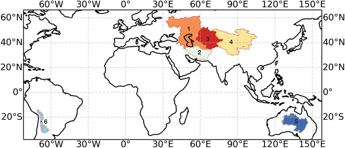
FIGURE 1. Location of selected endorheic basins. (1) Caspian Sea Basin, (2) Asia—west, (3) Aral Sea Basin, (4) Asia—east, (5) Central Australia region, and (6) Altiplano Plateau Basin.

The Caspian Basin covers an area of around 3.4 million km² and is located in Eurasia, bordered by five countries: Russia, Iran, Turkmenistan, Kazakhstan, and Azerbaijan. The basin consists of several sub-basins, including the Caspian Sea itself, which is the largest inland water body in the world. The majority of inflow to the Caspian Sea is derived from the Volga River, accounting for over 80% of the total, while the Kura and Ural rivers also contribute to its water supply (Dumont, 1998). There is a diverse range of climatic conditions across the region, with high precipitation over drainages to the north, but with minimal amounts toward the southeast.

Asia—west is situated below the Caspian Basin and covers large parts of southwestern Afghanistan and southeastern Iran, with a total area of 1,380,822 km². It includes basins such as the Sistan and the Iran inland rivers, which receive water from the Helmand River and are characterized by very low rainfall. The Sistan Basin serves as a crucial source of drinking water and plays a vital role in supporting agricultural activities. However, the basin faces significant challenges due to its low irrigation efficiency, posing a high threat to its sustainability (Mir et al., 2022).

The Aral Sea basin is located in Central Asia, primarily in Kazakhstan and Uzbekistan, covering approximately 1.9 million km². It contains the Aral Sea, Amu Darya River, and Syr Darya River, exhibits a climate that is predominantly continental and features desert and grassland regions (Berdimbetov et al., 2020). The basin contains several aquifers, including alluvial aquifers, in the Amu Darya and Syr Darya basins.

Asia—east lies adjacent to the Aral Sea Basin and comprises sub-basins such as the Tarim River Basin, the largest endorheic basin in China, and also the Mongolia Plateau Basin, Hexi Corridor Basin, Qiantang Plateau Basin, Qaidam Basin, Junggar Basin, Lake Balkhash, and the Turpan Basin. The whole area covers 5,091,542 km². The Tarim River Basin is known for its extensive aquifer systems. The basin contains both shallow and deep aquifers within its sedimentary rock formations. These aquifers play a vital role in sustaining water supplies for agriculture, industry, and human settlements in the region (Xia et al., 2019).

The Australian Basin, with a total area of 1,890,329 km², includes Lake Eyre which covers almost one-sixth of the country. It exhibits distinct rainfall patterns, with the northern and northeastern parts experiencing a summer-dominant rainfall regime, while the southern regions have a winter-dominant rainfall regime. The basin also experiences high potential evaporation rates. It contains two distinct aquifer systems: shallow alluvial aquifers connected to the surface water system and deep artesian aquifers within the Great Artesian Basin (Habeck-Fardy and Nanson, 2014).

The Altiplano Plateau Basin has an area of 537275 km² and lies in the Central Andes, covering parts of Bolivia, Chile, and Peru. It includes the Altiplano Basin, which is the largest endorheic basin in South America encompassing Lake Titicaca, Lake Poopo, and Salar de Uyuni (Canedo et al., 2016). The climate of the region is influenced by its high altitude and mountainous terrain, resulting in cool temperatures and variable precipitation patterns.

3 Methods

3.1 Flux-inferred storage

Petch et al. (2023) developed a method for comparing precipitation and evapotranspiration fluxes with GRACE surface water storage anomalies, defining a flux-inferred storage (FIS) that integrates the fluxes into and out of a region.

This takes the LHS (left hand side) of Eq. 1 and integrates it as follows, using precipitation and evapotranspiration observations,

S [0] is the GRACE total water storage anomaly at the beginning of our study period (January 2002) and is used to initialize the FIS time series. If the observations were in balance, then this FIS would be equivalent to the GRACE TWS time series, but instead, this quantity can highlight imbalances over both short and long timescales.

Figure 2 shows the GRACE storage along with the flux implied storage FIS from the initial precipitation and evapotranspiration based on Eq. 4. It can be seen that in all basins, there is a considerable divergence from the GRACE storage over the whole period. It can also be seen that the seasonal cycle in FIS is also often larger than seen in GRACE, e.g., in both Asia—east and Asia—west basins, indicating that there is insufficient cancellation between seasonal P and E variations. In this paper, we extended these FIS diagnostics to help attribute the variability in water storage detected by GRACE, over both seasonal and interannual timescales, as well as assessing contributions to storage trends over the 20 years of available GRACE data.

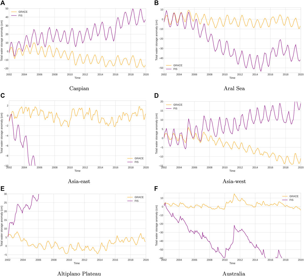
FIGURE 2. GRACE storage compared to the flux-inferred storage (FIS) from observations. (A) Caspian (B) Aral Sea (C) Asia-east (D) Asia-west (E) Altiplano Plateau (F) Australia.

3.2 Isolating storage contributions

In order to attribute the storage variations detected by GRACE to variations in the individual components of the hydrological budget, we produced two contributions to Eq. 4 based on integrating the precipitation and evapotranspiration observations separately. To compare these with the GRACE storage time series, we removed the time mean flux contribution and replaced it with the mean storage change from GRACE. Thus, for precipitation storage variations, we use the following formula:

where $\bar{P}$ is the mean precipitation and $\overline{dS}$ is the mean monthly storage change flux from GRACE. A similar calculation is performed using the evapotranspiration observations to produce FIS_E.

To quantify how much of the interannual variability can be explained by each of the flux contributions, we calculated the correlation between GRACE and the flux-inferred storages. To avoid correlation from the trend-matching, we forced the overall trend to be 0 for both GRACE and the FIS. Additionally, to avoid correlation signals from the seasonal cycle, we deseasonalized the storage by removing the monthly mean seasonal cycle. We also compared these mean seasonal cycles in a seperate analysis.

To assess trends in the fluxes, we looked at the annual mean P and dS based on the observations. Linear regression was used to quantify trends, with statistical significance assessed using a p-value of 0.05. Additionally, we calculated the total storage change over 18 years, resulting from these apparent trends, which were then compared with the total storage changes observed by GRACE over this period. Trends in E were not analyzed here due to the limited variations in E observations from year to year.

3.3 Energy

Following Petch et al. (2023), in the absence of surface energy storage data, we define the total energy storage anomaly constraint based on the flux observations according to Eq. 2. We first annually detrend NET so there is no gain or loss of energy over each year and then integrate over our time period initializing at 0. This generates a storage anomaly without any NET bias from the observations each year, which removes the interannual variability but still allows some variability in the seasonal storage cycle. This is then used as a total energy storage observation within F_obs in the budget closure calculation, described below. As this is only imposed as a weak constraint, the final closed budget solution can still retain some interannual energy storage variability, for example, imposed from the radiation variability or through variations from the coupled water cycle.

3.4 Closing budgets

To compare full consistency with the GRACE storage data, we can take the observed fluxes and adjust them to satisfy Eq. 1, accounting for the uncertainties of each component. The budget balancing was performed in a way that ensures consistency with GRACE on both short and long timescales (Petch et al., 2023). We also solved the energy budget simultaneously and coupled the two cycles through a shared latent heating term. To do this, we set up a cost function:

where F_obs is a vector of the observed fluxes, both water and energy, for month k and F is a vector of the budget-adjusted fluxes we seek. Uncertainties are contained in the error covariance matrix S_obs, which is a diagonal matrix representing the assumption that the errors between fluxes are uncorrelated. The monthly water budget is represented by vector A and imposed as a hard constraint using the Lagrange multiplier λ. The monthly energy budget is similarly represented by vector B, with the Lagrange multiplier μ. The cost function is minimized sequentially each month, which enables the fluxes to be consistent with GRACE water storage anomalies on all timescales. Further details can be found in Petch et al. (2023).

4 Results

4.1 Seasonal cycle

The time mean seasonal cycle of fluxes is defined by first removing the time mean and trend of the P and E fluxes and then calculating the mean seasonal cycle. Comparable mean monthly GRACE fluxes dS are calculated from the detrended GRACE storage. These trends will be compared later.

Figures 3, 4 show, on the left, the seasonal cycles of P, E, P − E and the monthly GRACE fluxes dS for all six endorheic basins we examined. The original data are shown as dashed lines, while the budget-adjusted seasonal cycles using Eq. 6 are shown as solid lines. The right of these figures shows the seasonal storage FIS contributions of P, − E and P − E, now compared directly with GRACE storage seasonal anomalies. These show smoother variations being integrals of the fluxes. It is of note here that the sign of FIS_E is reversed so that the P and E contributions to storage are additive. Again, the dashed lines represent the original data, while the solid lines represent the closed budget analyses using Eq. 6. Figure 3 shows basins with smaller seasonal cycles, and Figure 4 shows those basins with larger seasonal cycles using two different scales.

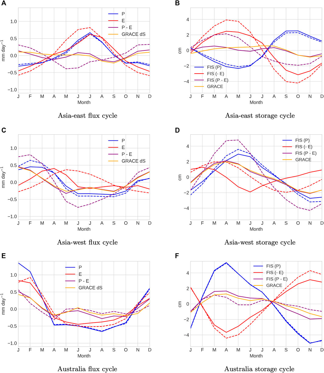
FIGURE 3. Mean seasonal flux cycles (left) and mean seasonal storage cycles (right). Original flux data are shown by dashed lines, and closed budget solutions are shown by solid lines. Includes basins with a smaller seasonal cycle, all using the same scale. (A) Asia-east flux cycle (B) Asia-east storage cycle (C) Asia-west flux cycle (D) Asia-west storage cycle (E) Australia flux cycle (F) Australia storage cycle.

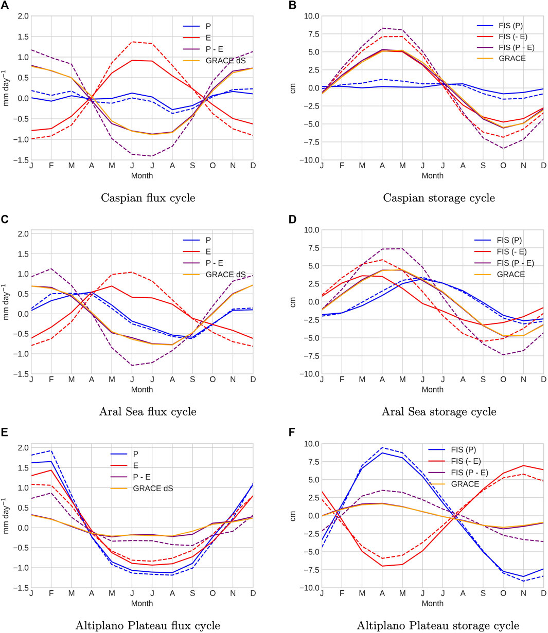
FIGURE 4. Mean seasonal flux cycles (left) and mean seasonal storage cycles (right). Original flux data are shown by dashed lines, and closed budget solutions are shown by solid lines. Includes basins with a larger seasonal cycle, all using the same scale. (A) Caspian flux cycle (B) Caspian storage cycle (C) Aral Sea flux cycle (D) Aral Sea storage cycle (E) Altiplano Plateau flux cycle (F) Altiplano Plateau storage cycle.

In the southern hemisphere Australian (Figures 3E,F) and Altiplano Plateau (Figures 4E,F) basins, the seasonal water storage cycle is clearly driven by P. Precipitation rises more rapidly than evaporation from October–January, Figures 3E, 4E, with the seasonal storage peaking in March–April, Figures 3F, 4F, before increasing evaporation reduces the storage. The P and E cycles are strongly canceling, although with P being larger, leading to a much smaller seasonal cycle in dS and S. The budget closure leads mainly to small adjustments in the evaporation cycles (increasing/decreasing amplitudes in Altiplano Plateau/Australia, respectively) without changing key features of the seasonal budgets.

The Caspian (Figures 4A,B) and Aral Sea (Figures 4C,D) basins exhibit very different seasonal storage variations primarily driven by evapotranspiration. In the Caspian Basin, there is very little variation in precipitation. Seasonal water storage peaks in April–May and declines sharply in June–July when seasonal evaporation reaches a maximum. The Aral Sea does have a seasonal precipitation cycle peaking in April, but this remains smaller than the evaporation cycle, and seasonal water storage shows similar variations to those of the neighboring Caspian, peaking in April–May, Figures 4B, D. The budget adjustments lead to significant weakening of the peak evaporation in both basins, required by the smaller seasonal water storage cycles seen in GRACE data, although the adjusted evaporation variations remain stronger than those of precipitation in controlling seasonal water storage.

The Asia—west basin (Figures 3C,D), covering mainly Iran and Afghanistan to the south of the Caspian and Aral basins, shows some common variability, although with substantially weaker variations in P and E. Precipitation peaks in February, with evaporation peaking later in April–May and water storage reaching a maximum in April. The variations in precipitation-driven storage are clearly larger now than those in the evaporation driven-storage in Figure 3D, which along with the timing of the peaks strongly suggest that the storage cycle is dominantly precipitation-driven, with evaporation playing a dampening role. The budget closure adjustments suggest reduced seasonal P and E amplitudes, an earlier evaporation peak in April with a much sharper decline into June, and no variability from June–January. Overall, these adjustments halve the seasonal water storage variability and bring the peak storage earlier to April, consistent with GRACE.

The Asia—east area to the east of the other Asian basins covers the high plateau of Tibet. Seasonal variations are weak but well-defined, with precipitation and evaporation both peaking in July. In the observations, the evaporation variations are larger, with a water storage peak in April, but after the budget closure adjustments, there is a close cancellation in P and E, leading to very little seasonal variation in water storage, as suggested by GRACE.

The effect of imposing seasonal budget closure against GRACE data mainly leads to evaporation adjustments in all these basins, as the observational uncertainties are larger than for P, and this usually leads to a reduction in the seasonal evaporation amplitudes as the GRACE water storage cycles show smaller variability than implied by the observed P − E; Figure 3; Figures 4B, D, F. The dominant driver of seasonal storage variability does change between basins, with the Caspian and Aral sea basins appearing to be dominated by evaporation variability on a seasonal timescale. We will compare this conclusion with the drivers of interannual storage variability in the next subsection.

4.2 Interannual variability

While P and E together determine the seasonal cycle in water storage in all these basins (apart from the Caspian Basin), the causes of interannual variability in water storage, which is clearly detectable in GRACE, are harder to measure.

To study the interannual variability, we use the FIS_P and FIS_E storage contributions, with the mean seasonal cycle and trends in fluxes removed, and compare these directly with the GRACE storage, also with the mean seasonal cycle and trends removed. These storage measures are less noisy than the flux variability and make attributing the drivers easier, as shown in Figure 5.

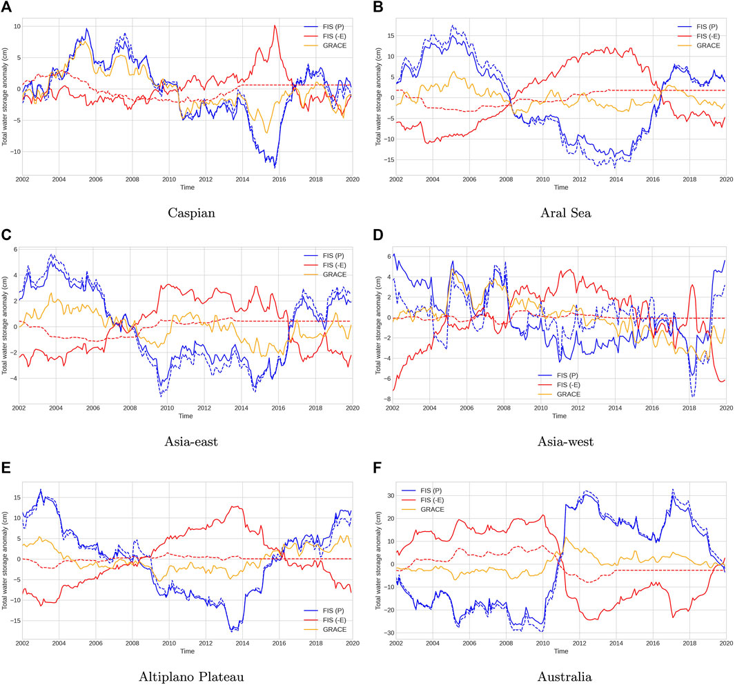
FIGURE 5. GRACE storage (orange), FIS_P (blue), and FIS_–E (red) after trends and mean seasonal cycle are removed. (A) Caspian (B) Aral Sea (C) Asia-east (D) Asia-west (E) Altiplano Plateau (F) Australia.

It is remarkable how much of the interannual storage variability detected by GRACE can be clearly attributed to variations in precipitation detected through the FIS_P metric in all these basins. In contrast, the original evapotranspiration data FIS_E show very little in the way of interannual variability, and wherever there are some FIS_E variations they are generally in a sense to dampen the interannual storage variations. This inability to capture interannual evapotranspiration can be attributed to inadequate observations. However, following budget closure, FIS_E displays greater variability, enhancing its storage dampening role.

To bring out these relationships, from Figure 5, a quantitative metric is obtained by correlating these storage time series, as shown in Table 1. Where there is a strong positive correlation between the observed FIS_P and GRACE storage, this supports precipitation being the key driver of the variability in storage. This correlation is as high as +0.88 in the Caspian Basin, and this is preserved in each basin after budget closure. All basins, apart from the Caspian, show negative FIS_P, FIS_E correlations, with the last column indicating compensating flux impacts on storage. The FIS_P−E correlations with GRACE become almost perfect after budget closure when fluxes fully explain the amplitudes and timings of interannual variability in storage observed by GRACE. It should be noted that, prior to budget closure, correlations with FIS_E only reflect the period 2002–2013 where FLUXCOM data are available.

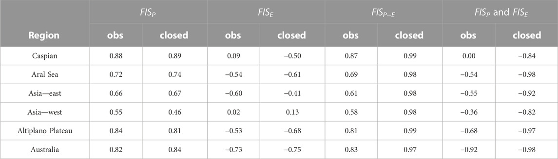
TABLE 1. Correlations between GRACE and flux-inferred water storages after trends and seasonal cycles are removed. Correlations are shown for storages inferred from observations (obs) and from closed budget estimates (closed). The last column shows the correlation between P- and E-driven storage variations. Bold values in Table “obs” and “closed” indicate the correlation with GRACE and the storage inferred from the—observed values (obs)—closed budget estimates (closed) i.e., after observations have been optimised to achieve water budget closure.

In the Asia—east region, during the period between 2004 and 2010, a significant reduction occurred in the FIS_P-driven storage, implying a loss of ∼8 cm (Figure 5C). However, the corresponding decline recorded by GRACE is only ∼4 cm. Although the original FIS_E values show few obvious signs of compensation, the adjusted FIS_E values show a decrease in evaporation during the same period, leading to a smaller total storage decline. Individual years where GRACE storage increases/declines are also seen to be driven by a correspondingly larger increase/decrease in FIS_P, e.g., 2003–2004 or 2009. There is a +0.66 correlation of FIS_P, and a -0.60 correlation of FIS_E, with GRACE prior to budget closure, clearly indicating the driving role of precipitation and the dampening role of evaporation in water storage changes.

In the Aral Sea Basin, the FIS_P reproduces the higher frequency, annual timescale, and variations in the GRACE storage very well in both amplitude and timing. A marker of this is how little annual variability appears in the FIS_E after budget closure. The original FIS_P correlation with GRACE is now +0.72. The impact of the budget closure is primarily on longer, multi-year timescales. The FIS_P reproduces the multi-year variability in GRACE storage but at a considerably higher amplitude, e.g., the 13-cm FIS_P increase from January 2002 to March 2005, compared with the 8.2 cm increase in GRACE (Figure 5B). In addition, on longer timescales from March 2005 to December 2013, FIS_P declines by 30 cm, compared with a 10 cm decline in GRACE. This indicates the strong dampening of storage variability from E variations. There is some evidence in the observed FIS_E, which clearly anti-correlates (−0.54) with FIS_P, but the amplitude changes of ∼5 cm are much too small to explain the FIS_P, GRACE discrepancy. After budget closure, FIS_E shows a much stronger dampening of multi-year FIS_P-driven changes (correlation −0.98), such that the GRACE storage variations are also reproduced at the correct amplitude. The variability of FIS_P also slightly reduces after budget closure. This is similar to what we observe in Asia–east, which is not unexpected due to the close proximity of these regions.

Similar to the Aral Basin, in the Caspian Sea Basin, FIS_P is able to explain both the annual and multi-annual variations in the GRACE storage particularly well, with FIS_P, and GRACE correlations up at +0.88. This is a very clear indication that on annual-to-multi-annual timescales, precipitation is the dominant driver of the storage variability seen in GRACE. This is perhaps particularly surprising for the Caspian and Aral basins because the seasonal variations in water storage are very clearly dominated by E variability, Figure 4. There is minimal dampening from FIS_E on both annual and multi-annual timescales, shown by negligible correlations of FIS_E with GRACE, indicating that both the phase and amplitudes of the Caspian storage variations are mostly very well-explained by precipitation variability, except in 2014–2016 when, after budget closure, the strong decline in precipitation is accompanied by reduced evaporation, partly mitigating the impact on water storage (Figure 5A).

The Asia–west basin seems to display mixed driving of storage changes. There are years with very strong precipitation-driven storage peaks, e.g., 2005 and 2007, and periods when smaller subannual storage peaks appear to be precipitation-driven, 2003, 2014–2017 (Figure 5D). However, there are some multi-year periods when storage seems mainly E-driven, e.g., 2008–2010, and the steady decline from 2012 to 2018. It is notable that this basin also shows more complex seasonal cycle behavior as observed in Figures 3C,D. The FIS_P correlation with GRACE at +0.55 is the lowest of any basin, and after budget closure, this declines, and the FIS_E correlation with GRACE becomes slightly more positive, suggesting that evaporation is indeed responsible for driving at least some of the storage variability.

In Australia, we see a clear pattern in each of the storage contributions as a result of the 2010–2012 La Niña event, which was one of the strongest on record. There is a significant increase in FIS_P, equivalent to over 50 cm excess storage (Figure 5F). This huge event is also captured by the observed FIS_E, with an additional evaporation of approximately 16 cm. However, this insufficiently reduces the FIS_P gain. The budget closure against GRACE enhances the FIS_E dampening of P-driven storage changes, during this large La Niña event as well as in other periods, e.g., dampening the larger annual storage cycles in 2005 and 2008. The precipitation mostly remains unchanged during budget closure, except for slightly reduced maxima and minima storage values. The FIS_P and FIS_E are +0.82 and −0.73 correlated with GRACE storage, respectively.

In the Altiplano Plateau Basin, we also observe some distinctive patterns in FIS_P. There is a large multi-annual decline from 2003 to 2014, followed by a recovery period characterized by an increase until 2020 (Figure 5E). This low-frequency variability is clearly reflected in the GRACE storage, although with considerably smaller changes. Much of the year-to-year variability in FIS_P is also evident in GRACE, e.g., the maximum variability in 2003. Although the observed FIS_E exhibits only small variability, there are indications of reduced evaporation from 2003 to 2013, which aligns with the period of reduced precipitation; however, these changes are much too small to dampen the interannual P-driven storage. Once budget closure constraints are applied, the interannual E variability increases, dampening the impact of P variability and giving close agreement with GRACE storage. The FIS_P and FIS_E are +0.84 and −0.53 correlated with GRACE storage, respectively.

4.3 Trends

Only two of the basins studied show robust downward water storage trends in the GRACE data: the Caspian Basin and the adjacent Asia—west basin, as can be seen in Figure 2. We were careful to remove trending information from the seasonal and interannual variability comparisons described previously. It might be natural to attribute trends to the same drivers as the aforementioned interannual variability, the trend being a sample of longer timescale variations. However, the original precipitation and evaporation flux datasets are fundamentally out of balance, preventing any causal inferences from being obtained from this time mean imbalance. Instead, we can ask if anything has changed during the study period, which might contribute to a storage trend. From Eq. 1, trends in storage changes, dS, must reflect trends in precipitation and/or evaporation. Trends in dS would then indicate a strengthening or dampening of the GRACE S storage trends. Figure 6 shows the annual mean precipitation and GRACE dS values over the 18-year period. The Caspian, Aral, and Asia—west basins show small downward trends in dS (Figures 6A,B,D), while the Altiplano Plateau Basin shows an upward trend (Figure 6E). Only the Caspian and Altiplano Plateau basins have precipitation trends of the same sign, in both cases more than sufficient to explain the dS trends (neglecting evaporation trends which are undetectable in FLUXCOM), although none of these trends is significant given interannual variability. The strong interannual correlations noted in Figure 5 are clearly seen again in Figure 6.

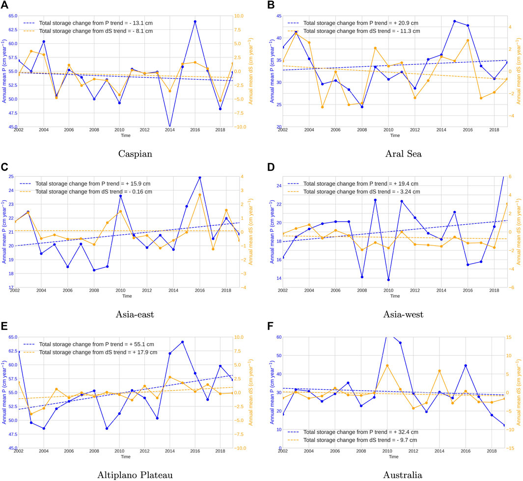
FIGURE 6. Annual mean precipitation (P) and storage changes (dS) over the 18-year period of data (left and right axes, respectively). Trend lines are shown, and the total 18-year storage changes implied by these trends are shown in the inset text. (A) Caspian (B) Aral Sea (C) Asia-east (D) Asia-west (E) Altiplano Plateau (F) Australia.

The inset text Figure 6 give the 18-year storage changes resulting from the assessed trends. For the Caspian, this explains 70% of the 18-year storage changes (−10.7 cm) seen in Figure 2. For Asia—west, the precipitation trend is positive, although again no significance can be attached. It is notable that, unlike the Caspian, the interannual variability in Asia—west storage is only fairly weakly correlated with precipitation, given in Table 1. It has been suggested that groundwater extraction (which would become evaporation) is a major contributor to storage decline here (Nazari et al., 2023), and its intensification over the 2002–2020 period may explain the increasingly negative dS over the period.

4.4 Energy storage

Figure 7 shows the total energy storage anomalies implied from both the raw observations (blue) and the new estimates after budget closure (green). It is clear that the observations initially contain large imbalances, as the blue dashed line diverges very quickly in most basins, caused by a positive bias in the NET flux. The exceptions are the Aral Sea and Australia, where the energy FIS exhibits more interannual variability. In the Aral Sea (Figure 7B), the observations suggest a significant decline in energy storage from 2006–2016, which coincides (although slightly delayed) with the decrease in FIS_P and increase in FIS_E seen in Figure 5B. This would be consistent with dryer surface conditions and a reduced surface heat capacity. In Australia, the observations show an increase in energy storage from 2010–2012 and then a decline from 2012 to 2016, due to the large La Niña event and its aftermath, following a similar pattern to what is seen in water storage. These features are still present, but considerably dampened after budget closure, as the yearly energy budget balance weak constraint is being applied.

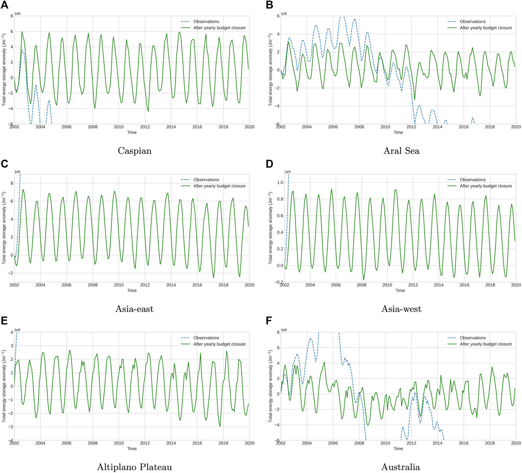
FIGURE 7. Energy storage inferred from optimized estimates (green) and storage inferred from raw observations (blue dashed lines). (A) Caspian (B) Aral Sea (C) Asia-east (D) Asia-west (E) Altiplano Plateau (F) Australia.

Table 2 shows the anomaly correlation between the NET flux and its constituent parts after budget closure. These correlations provide insight into the factors driving the interannual variability in the energy storage anomaly. Radiation is always positively correlated and is the primary driver, while the latent heat, with negative correlations, is usually dampening NET variations. Much of the interannual latent variability is developed through water budget closure, which FIS_E also exhibits a strong negative correlation with GRACE water storage. Further investigation of the energy and water budget interactions should be a topic for further work.

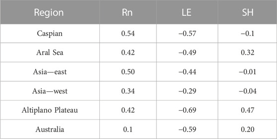
TABLE 2. Flux anomaly correlations with NET surface energy flux after budget closure. The mean seasonal cycles have been removed from each flux. Rn represents the total radiative fluxes.

5 Discussion

The initial time mean imbalance in the water budget calculated from precipitation and evaporation observational data is relatively large in all basins, ranging between 21% and 45% of mean precipitation. These imbalances mean we are unable to sensibly attribute any of the long-term storage trends seen by GRACE. Although P and E are fundamentally out of balance, they are still able to provide some insight into the seasonal and interannual variability of GRACE.

Overall, we find the observations suggest that precipitation is a key control of the interannual storage variability. This is particularly evident in the Caspian Sea Basin, which is consistent with findings from Rodell et al. (2018). The study notes that interannual variations in discharge from the Volga River (which is contained in the Caspian Sea Basin) are driven by changes in precipitation and exhibit a magnitude nearly three times larger than that of the interannual variations in evaporation. Additionally, they find that the annual discharge from the Volga River explains 60% of the variance in the annual mean level of the Caspian Sea compared with only 18% explained by evaporation.

In the Altiplano Plateau Basin, the FIS_P metric clearly highlights a precipitation deficit from 2003 to 2013, which directly contributes to the loss of storage over this period. Wang et al. (2018) discussed the extensive impact of this precipitation deficit in the Dry Andes and Patagonia, which, in conjunction with human activities, has resulted in concurrent losses across multiple water stores. Wang et al. (2018) also note that by the end of their 2002–2016 study period, the storage decline showed signs of slowing down and has partially reversed by 2012. The inclusion of more recent GRACE data enables us to observe a full recovery in storage back to the levels observed in 2002–2004 over the 2014–2020 period, which is largely due to increased precipitation, indicated clearly by the FIS_P.

Over the Aral Sea Basin, Zmijewski and Becker (2014) found a slight increase in precipitation from 2000 to 2010 using Tropical Rainfall Measuring Mission and GPCC data, although they did not claim this as significant. In contrast to this increase in precipitation, they found that dS showed signs of decreasing, which they attributed to increased evaporation resulting from anthropogenic modification, particularly due to inefficient irrigation in the upstream region. Hu et al. (2022) found similar trends over the Aral Sea Basin in the period 2003–2016. They found increasing trends in annual P and E, while the storage anomalies showed a decreasing trend, with values ranging from −0.47 mm/month to −0.29 mm/month.

In arid regions such as the Aral Sea Basin, Wei et al. (2013) demonstrated that irrigation-induced water loss through evapotranspiration is typically significantly greater than the local increase in precipitation caused by irrigation. As a result, the region experiences a net water deficit. Our results in Section 6 also show short-term trends in P and dS over our study period; however, the FIS_P in Figure 5 clearly illustrates that P increases until 2005, but then there is a strong decline through 2010. Comparison with GRACE dS is consistent with both the initial rise and subsequent decrease over this period. This indicates that the precipitation observations are capable of effectively explaining the observed storage variations during this period. This is in agreement with Hu et al. (2022), who conclude that precipitation has a major impact on interannual variations of all terrestrial water cycle components over the Aral Sea Basin, including storage anomalies, groundwater, and soil moisture. Additionally, they state that the effects of evapotranspiration on these components are primarily influenced by the amount of precipitation received. Our results also agree with those of Hu et al. (2021), who found that precipitation has a larger influence over storage variations than evapotranspiration over Central Asia, which includes the Aral Sea Basin and a significant portion of Asia—east.

Throughout the study period from 2002 to 2020, Australia experienced a number of hydroclimatic extremes directly influenced by the El Niño Southern Oscillation (ENSO) and the Indian Ocean Dipole (IOD) (Cai et al., 2011). The endorheic basin investigated here is primarily located within the zone where TWS is mainly driven by ENSO (Xie et al., 2019). From 2002 to 2009 Australia faced severe drought (Yang et al., 2017a); however, from 2010 to 2012, the water storage in most parts of Australia was replenished. Xie et al. (2015) found that this was primarily due to La Niña, with 2 years of significantly higher-than-normal precipitation in 2010 and 2011 (Boening et al., 2012). Our results strongly agree with the importance of precipitation in driving the variability of water storage. In Figure 5F, the FIS_P clearly demonstrates distinct drying and wetting phases, which are correlated with GRACE storage variability but which are also dampened by evaporation variations. Our findings also support the notion from Xie et al. (2019) that across Australia, water resources are characterized by rapid replenishment following wet events, but much more gradual depletion.

The budget closure approach implemented here shares similarities to those of other studies, such as Liu (2022a,b); Liu et al. (2016), which simulate evaporation estimates based on the water balance method, without using any independent evaporation data. To do this, each of these studies uses an ensemble of estimates for both P and dS. Although we only use a single data source as input, the budget closure has the benefit of allowing P and dS observations to adjust according to their relative uncertainties, which take into account the spread of other products.

The effects of budget closure are primarily evident in the adjustments made to E, given the larger uncertainties associated with the observations. In most cases, we see that E closely responds to variations in P, while usually maintaining the overall phase of the seasonal cycle. In the Asia—west region, however, the peak in E shifts from May to April. This phase shift agrees with the simulated evaporation estimates from Liu (2022b), which also show a peak in April for the Helmand River Basin.

The original evaporation data showed limited variability, so a greater emphasis was placed on the GPCP and GRACE observations for this study. Extending the FLUXCOM time series with the mean seasonal cycle allowed us to explore and comprehensively analyze the variations in precipitation and storage that occurred from 2014 to 2020. Given the low interannual variability seen in turbulent energy flux data, we believe the extension of the FLUXCOM time series does not significantly impact the results. During this period, increased uncertainties meant that the E estimates produced after budget closure were more strongly adjusted. While this introduces some limitations to our study, previous research has often simply estimated E as a residual of other observations. A further limitation is the lack of availability of groundwater data representative of our study regions. While it would be useful to compare groundwater withdrawal trends with GRACE observations, the lack of accessible data, along with its unsuitability for large-scale analysis, restricts its inclusion in this study.

Our water budget findings can stand independent of the coupled energy budget, as only minimal energy constraints were imposed which did not significantly impact the water budget components during budget closure. However, we primarily included energy budget analysis in our study because it provides a framework that can be extended in the future with the inclusion of additional data to provide monthly constraints.

6 Conclusion

This paper analyzed water storage variations in several endorheic basins using GRACE data from 2002 to 2020. We investigated seasonal storage variations, interannual variability, and longer-term trends while evaluating the ability of precipitation and evapotranspiration observations to explain these features. The paper considered raw observational data as well as data adjusted through inverse modeling to guarantee closed coupled water and energy budgets on monthly timescales, using methods from Petch et al. (2023), following Hobeichi et al. (2020) and L’Ecuyer et al. (2015). The energy balance allows varying year-to-year seasonal amplitude controlled by different energy flux components, in particular latent heat variations coupled to the water cycle. These could perhaps be verified against reanalysis or land surface temperature data, but we have left a full energetic analysis for future work. This paper focuses primarily on the attribution of GRACE water storage changes to variations in precipitation and evapotranspiration on different timescales.

Most basins show a seasonal cycle in surface water storage that is driven by precipitation; however, the water storage amplitudes are much smaller than those implied by precipitation alone. Generally, evapotranspiration increases and decreases with precipitation to dampen the storage changes, and in some basins, such as Asia—east, this results in virtually no seasonal variations in water storage at the surface. Generally, the seasonal evaporation taken from FLUXCOM is too strong in several basins, and the budget closure then leads to weaker variations in the seasonal evaporation to agree with GRACE.

The Caspian Basin is somewhat unusual in that the seasonal cycle in water storage appears to be driven by evaporation alone, with precipitation showing much smaller seasonal variability. This is partly the result of the large basin size as the seasonal precipitation in the northern and southern portions had some variation in anti-phase.

Most basins show considerable interannual variability in water storage over the 18 years of GRACE data. This study found that the main cause of these variations was nearly always precipitation variability. We attribute these storage changes after a process of deseasonalizing and detrending the data, which was then compared with the GRACE storage and the storage implied by integrating the precipitation and evaporation data into separate interannual time series. It is remarkable how well precipitation variability explains the GRACE storage variability. As mentioned, the variability implied by precipitation alone is usually larger than that detected by GRACE. The interannual variability in evaporation is now generally far too weak to explain this discrepancy, although there are some small indications of a dampening role in the FLUXCOM data. When budget adjustment is used, the evaporation variations become very clearly anti-correlated with precipitation to give a much better fit to the GRACE-measured storage.

The Caspian Basin variability is especially noteworthy. In the Caspian, the independent precipitation-driven storage variations match the GRACE data extremely well (correlating at +0.88 before budget closure), both on year-to-year and multi-year timescales. For example, the decline in GRACE storage between 2007 and 2011 is very well-captured, see Figure 5. This is despite the dominant role of evaporation being responsible for the seasonal changes in the basin. This very clear link between precipitation and multi-annual storage changes in all these basins is the most remarkable result here and perhaps challenges climate model inferences regarding the causes of long-term changes in water availability as being due to evaporation increases in a warmer climate, e.g., Chen et al. (2017). The observations of evaporation do not independently support such low-frequency changes.

We cannot attribute linear trends in GRACE storage, which depend on constant differences between precipitation and evaporation that are typically highly out of balance in the initial data, as seen in Figure 2. However, we have looked for 18-year trends in precipitation, evaporation, and monthly storage changes, which should also be in balance. Over the Caspian, in particular, there is a downward trend in precipitation, which is more than sufficient to explain a downward trend in storage, and without any initial imbalance in P − E this trend is still sufficient to explain 70% of the GRACE total storage loss over 18 years. Although these trends are not statistically significant, given the amplitude of the interannual variability, they are consistent with the conclusion, based on interannual variations, that precipitation is the dominant driver in low-frequency storage changes in the Caspian Basin.

In future work, it would be valuable to better quantify the storage footprint characteristics resulting from rainfall anomalies in different basins, including the proportion of rainfall going into storage and the storage duration timescales. These storage responses differ across basins and may also vary with the temporal duration of the rainfall anomalies. Understanding how much water storage is retained and over what timescales will provide valuable insights into the hydrological dynamics of these basins and be beneficial for water resource management and decision-making, as it can help in assessing the resilience and sustainability of water systems under changing climatic conditions.

Data availability statement

The raw data supporting the conclusion of this article will be made available by the authors, without undue reservation.

Author contributions

This work was carried out by SP as a contribution to their Ph.D. The analyses and figures were generated by SP as were all drafts of the manuscript. KH, TQ, and RK acted as Ph.D. supervisors, BD helped with data acquisition and analysis, and each contributed edits to the manuscript. All authors contributed to the article and approved the submitted version.

Funding

This work was supported by the NERC DTP SCENARIO program and by a CASE award from the UK Met Office for SP. KH, TQ, and BD would also like to acknowledge the support of the NERC NCEO International Program (NE/X006328/1) for their contributions to this work.

Acknowledgments

This work is a contribution to the Ph.D. studies of SP and will be submitted as a contribution to their Ph.D.

Conflict of interest

The authors declare that the research was conducted in the absence of any commercial or financial relationships that could be construed as a potential conflict of interest.

Publisher’s note

All claims expressed in this article are solely those of the authors and do not necessarily represent those of their affiliated organizations, or those of the publisher, the editors and the reviewers. Any product that may be evaluated in this article, or claim that may be made by its manufacturer, is not guaranteed or endorsed by the publisher.

References

Adler, R. F., Huffman, G. J., Chang, A., Ferraro, R., Xie, P., Janowiak, J., et al. (2003). The version-2 global precipitation climatology project (GPCP) monthly precipitation analysis (1979-present). J. Hydrometeor 4, 1147–1167. doi:10.1175/1525-7541(2003)004<1147:tvgpcp>2.0.co;2
Adler, R., Wang, J.-J., Sapiano, M., Huffman, G., Chiu, L., Xie, P. P., et al. (2016). Global precipitation climatology project (gpcp) climate data record (cdr). North Carolina: national centers for environmental information.
Aires, F. (2014). Combining datasets of satellite-retrieved products. part i: Methodology and water budget closure. J. Hydrometeorol. 15, 1677–1691. doi:10.1175/JHM-D-13-0148.1
Berdimbetov, T., Ma, M., Liang, C., and Ilyas, S. (2020). Impact of climate factors and human activities on water resources in the Aral Sea basin. Hydrology 7, 30. doi:10.3390/hydrology7020030
Boening, C., Willis, J. K., Landerer, F. W., Nerem, R. S., and Fasullo, J. (2012). The 2011 La Niña: So strong, the oceans fell. Geophys. Res. Lett. 39, a–n. doi:10.1029/2012GL053055
Boergens, E., Kvas, A., Eicker, A., Dobslaw, H., Schawohl, L., Dahle, C. e. a., et al. (2022). Uncertainties of GRACE-based terrestrial water storage anomalies for arbitrary averaging regions. JGR Solid Earth 127, e2021JB022081. doi:10.1029/2021JB022081
Cai, W., van Rensch, P., Cowan, T., and Hendon, H. (2011). Teleconnection pathways of enso and the iod and the mechanisms for impacts on Australian rainfall. J. Clim. 24, 3910–3923. doi:10.1175/2011JCLI4129.1
Canedo, C., Pillco Zolá, R., and Berndtsson, R. (2016). Role of hydrological studies for the development of the tdps system. Water 8, 144. doi:10.3390/w8040144
Chen, J., Cazenave, A., Dahle, C. e. a., Llovel, W., Panet, I., Pfeffer, J., et al. (2022). Applications and challenges of grace and grace follow-on satellite gravimetry. Surv. Geophys 43, 305–345. doi:10.1007/s10712-021-09685-x
Chen, J. L., Pekker, T., Wilson, C. R., Tapley, B. D., Kostianoy, A. G., Cretaux, J.-F., et al. (2017). Long-term Caspian Sea level change. Geophys. Res. Lett. 44, 6993–7001. doi:10.1002/2017GL073958
Dumont, H. J. (1998). The caspian lake: History, biota, structure, and function. Limnol. Oceanogr. 43, 44–52. doi:10.4319/lo.1998.43.1.0044
Gaybullaev, B., Chen, S., and Gaybullaev, D. (2012). Changes in water volume of the aral sea after 1960. Appl. Water Sci. 2, 285–291. doi:10.1007/s13201-012-0048-z
Habeck-Fardy, A., and Nanson, G. C. (2014). Environmental character and history of the lake eyre basin, one seventh of the Australian continent. Earth-Science Rev. 132, 39–66. doi:10.1016/j.earscirev.2014.02.003
Hobeichi, S., Abramowitz, G., and Evans, J. (2020). Conserving land-atmosphere Synthesis suite (CLASS). J. Clim. 33, 1821–1844. doi:10.1175/jcli-d-19-0036.1
Hu, Z. Y., Chen, X., Zhou, Q. M., Yin, G., and Liu, J. (2022). Dynamical variations of the terrestrial water cycle components and the influences of the climate factors over the aral sea basin through multiple datasets. J. Hydrology 604, 127270. doi:10.1016/j.jhydrol.2021.127270
Hu, Z. Y., Zhang, Z. Z., Sang, Y. F., Qian, J., Feng, W., Chen, X., et al. (2021). Temporal and spatial variations in the terrestrial water storage across central Asia based on multiple satellite datasets and global hydrological models. J. Hydrology 596, 126013. doi:10.1016/j.jhydrol.2021.126013
Huang, J., Yu, H., Guan, X., Wang, G., and Guo, R. (2016). Accelerated dryland expansion under climate change. Nat. Clim. Change 6, 166–171. doi:10.1038/nclimate2837
Jung, M., Koirala, S., Weber, U. e. a., Ichii, K., Gans, F., Camps-Valls, G., et al. (2019). The fluxcom ensemble of global land-atmosphere energy fluxes. Sci. Data 6, 1. doi:10.1038/s41597-019-0076-8
Kato, S., Rose, F. G., Rutan, D. A., Thorsen, T. E., Loeb, N. G., Doelling, D. R., et al. (2018). Surface irradiances of edition 4.0 clouds and the earth's radiant energy system (CERES) energy balanced and filled (EBAF) data product. J. Clim. 31, 4501–4527. doi:10.1175/JCLI-D-17-0523.1
Koriche, S. A., Singarayer, J. S., and Cloke, H. L. (2021). The fate of the caspian sea under projected climate change and water extraction during the 21st century. Environ. Res. Lett. 16, 094024. doi:10.1088/1748-9326/ac1af5
L’Ecuyer, T. S., Beaudoing, H. K., Rodell, M., Olson, W., Lin, B., Kato, S., et al. (2015). The observed state of the energy budget in the early twenty-first century. J. Clim. 28, 8319–8346. doi:10.1175/JCLI-D-14-00556.1
Liu, W., Wang, L., Zhou, J., Li, F. S., Sun, G., Fu, X., et al. (2016). A worldwide evaluation of basin-scale evapotranspiration estimates against the water balance method. J. Hydrology 538, 82–95. doi:10.1016/j.jhydrol.2016.04.006
Liu, X., Liu, Z., and Wei, H. (2022). Trends of terrestrial water storage and actual evapotranspiration in Chinese inland basins and their main affecting factors. Front. Environ. Sci. 10, 1. doi:10.3389/fenvs.2022.963921
Liu, Z. (2022a). Causes of changes in actual evapotranspiration and terrestrial water storage over the eurasian inland basins. Hydrol. Process. 36, e14482. doi:10.1002/hyp.14482
Liu, Z. (2022b). Evaluation of remotely sensed global evapotranspiration data from inland river basins. Hydrol. Process. 36, :e14774. doi:10.1002/hyp.14774
Loeb, N., Doelling, D., Wang, H., Su, W., Nguyen, C., Corbett, J., et al. (2018). Clouds and the earth’s radiant energy system (ceres) energy balanced and filled (ebaf) top-of-atmosphere (toa) edition-4.0 data product. Journal of Climate 31 (2), 895–918. doi:10.1175/JCLI-D-17-0208.1
Mayer, J., Mayer, M., Haimberger, L., and Liu, C. (2022). Comparison of surface energy fluxes from global to local scale. J. Clim. 35, 4551–4569. doi:10.1175/JCLI-D-21-0598.1
Mir, R., Azizyan, G., Massah, A., and Gohari, A. (2022). Fossil water: Last resort to resolve long-standing water scarcity? Agric. Water Manag. 261, 107358. doi:10.1016/j.agwat.2021.107358
Mohamed, A., Abdelrahman, K., and Abdelrady, A. (2022a). Application of time-variable gravity to groundwater storage fluctuations in Saudi Arabia. Front. Earth Sci. 10, 1. doi:10.3389/feart.2022.873352
Mohamed, A., Faye, C., Othman, A., and Abdelrady, A. (2022b). Hydro-geophysical evaluation of the regional variability of Senegal's terrestrial water storage using time-variable gravity data. Remote Sens. 14, 4059. doi:10.3390/rs14164059
Munier, S., Aires, F., Schlaffer, S., Prigent, C., Papa, F., Maisongrande, P., et al. (2014). Combining data sets of satellite-retrieved products for basin-scale water balance study: 2. Evaluation on the Mississippi basin and closure correction model. J. Geophys. Res. Atmos. 119, 12,100–12,116. doi:10.1002/2014jd021953
Nazari, A., Zaryab, A., and Ahmadi, A. (2023). Estimation of groundwater storage change in the helmand river basin (Afghanistan) using grace satellite data. Earth Sci. Inf. 16, 579–589. doi:10.1007/s12145-022-00899-0
Othman, A., Abdelrady, A., and Mohamed, A. (2022). Monitoring mass variations in Iraq using time-variable gravity data. Remote Sens. 14, 3346. doi:10.3390/rs14143346
Pan, M., Sahoo, A., Troy, T., Vinukollu, R., Sheffield, J., and Wood, E. (2012). Multisource estimation of long-term terrestrial water budget for major global river basins. J. Clim. 25, 3191–3206. doi:10.1175/jcli-d-11-00300.1
Pavelsky, T. (2018). World's landlocked basins drying. Nat. Geosci. 11, 892–893. doi:10.1038/s41561-018-0269-3
Petch, S., Dong, B., Quaife, T., King, R. P., and Haines, K. (2023). Water and energy budgets over hydrological basins on short and long timescales. Hydrol. Earth Syst. Sci. 27, 1723–1744. doi:10.5194/hess-27-1723-2023
Rodell, M., Beaudoing, H., L’Ecuyer, T., Olson, W., Famiglietti, P., and AdlerAdler, R. (2015). The observed state of the water cycle in the early twenty-first century. J. Clim. 28, 8289–8318. doi:10.1175/jcli-d-14-00555.1
Rodell, M., Famiglietti, J. S., Chen, J., Seneviratne, S., Viterbo, P., Holl, S. L., et al. (2004). Basin scale estimates of evapotranspiration using grace and other observations. Geophys. Res. Lett. 31, L2050. doi:10.1029/2004gl020873
Rodell, M., Famiglietti, J., Wiese, D. e. a., Reager, J. T., Beaudoing, H. K., Landerer, F. W., et al. (2018). Emerging trends in global freshwater availability. Nature 557, 651–659. doi:10.1038/s41586-018-0123-1
Rowlands, D. D., Luthcke, S. B., McCarthy, J. J., Klosko, S. M., Chinn, D. S., Lemoine, F. G., et al. (2010). Global mass flux solutions from grace: A comparison of parameter estimation strategies-mass concentrations versus Stokes coefficients. J. Geophys. Res. 115, 7B01403. doi:10.1029/2009jb006546
Save, H., Bettadpur, S., and Tapley, B. D. (2016). High-resolution CSR GRACE RL05 mascons. J. Geophys. Res. Solid Earth 121, 7547– 7569. doi:10.1002/2016JB013007
Scanlon, B. R., Zhang, Z., Save, H., Wiese, D. N., Landerer, F. W., Long, D., et al. (2016). Global evaluation of new grace mascon products for hydrologic applications. Water Resour. Res. 52, 9412– 9429. doi:10.1002/2016WR019494
Tapley, B. D., Bettadpur, S., Ries, J. C., Thompson, P. F., and Watkins, M. M. (2004). Grace measurements of mass variability in the Earth system. Science 305, 503–505. doi:10.1126/science.1099192
Trenberth, K. E., and Fasullo, J. T. (2013). Regional energy and water cycles: Transports from ocean to land. J. Clim. 26, 7837–7851. doi:10.1175/JCLI-D-13-00008.1
Vishwakarma, B. D., Bates, P., Sneeuw, N., Westaway, R. M., and Bamber, J. L. (2021). Re-assessing global water storage trends from grace time series. Environ. Res. Lett. 16, 034005. doi:10.1088/1748-9326/abd4a9
Wang, J., Song, C., Reager, J. e. a., Yao, F., Famiglietti, J. S., Sheng, Y., et al. (2018). Recent global decline in endorheic basin water storages. Nat. Geosci. 11, 926–932. doi:10.1038/s41561-018-0265-7
Wei, J., Dirmeyer, P. A., Wisser, D., Bosilovich, M. G., and Mocko, D. M. (2013). Where does the irrigation water go? An estimate of the contribution of irrigation to precipitation using merra. J. Hydrometeor. 14, 275–289. doi:10.1175/jhm-d-12-079.1
Wielicki, B. A., Barkstrom, B. R., Harrison, E. F., Lee, R. B., Louis Smith, G. L., and Cooper, J. E. (1996). Clouds and the earth's radiant energy system (CERES): An earth observing system experiment. Bull. Amer. Meteor. Soc. 77, 853–868. doi:10.1175/1520-0477(1996)077<0853:catere>2.0.co;2
Xia, J., Wu, X., Zhan, C., Qiao, Y., Hong, S., Yang, P., et al. (2019). Evaluating the dynamics of groundwater depletion for an arid land in the tarim basin, China. Water 11, 186. doi:10.3390/w11020186
Xie, Z., Huete, A., Restrepo-Coupe, N., Devadas, J., Davies, S., Waston, E., et al. (2015). Terrestrial total water storage dynamics of Australia's recent dry and wet events. Remote Sens. Environ. 231, 1. doi:10.1109/IGARSS.2015.7325935
Xie, Z., Huete, A., Restrepo-Coupe, N., Devadas, R., and Waston, C. (2015). “Terrestrial total water storage dynamics of Australia's recent dry and wet events,” in IEEE International Geoscience and Remote Sensing Symposium (IGARSS), Milan, Italy, 16 - 21 July, 2023 (IEEE), 992. doi:10.1109/IGARSS.2015.7325935
Yang, Y., McVicar, T. R., Donohue, R. J., Zhang, Y., Roderick, M. L., Chiew, F. H., et al. (2017a). Lags in hydrologic recovery following an extreme drought: Assessing the roles of climate and catchment characteristics. Water Resour. Res. 53, 4527–5197. doi:10.1002/2017WR020683
Yapiyev, V., Sagintayev, Z., Inglezakis, V., and Samarkhanov, K. (2017). Essentials of endorheic basins and lakes: A review in the context of current and future water resource management and mitigation activities in central Asia. Water 9, 798. doi:10.3390/w910079
Yu, L., Jin, X., and Weller, R. A. (2008). Multidecade global flux datasets from the objectively analyzed air-sea fluxes (oaflux) project: Latent and sensible heat fluxes, ocean evaporation, and related surface meteorological variables. United states: Woods Hole Oceanographic Institution, 64.
Zhang, G., Yao, T., Shum, C. K., Yi, S., Yang, K., Xi, H., et al. (2017). Lake volume and groundwater storage variations in Tibetan plateau’s endorheic basin. Geophys. Res. Lett. 44, 5550–5560. doi:10.1002/2017GL073773
Zhang, Y., Pan, M., Sheffield, J., Siemann, A., Fisher, C., Liang, M., et al. (2018). A climate data record (cdr) for the global terrestrial water budget: 1984–2010. Hydrology earth Syst. Sci. 22, 2125–2136. doi:10.5194/hess-22-241-2018
Zhao, K., and Li, X. (2016). Estimating terrestrial water storage changes in the tarim river basin using grace data. Geophys. J. Int. 211, 1449–1460. doi:10.1093/gji/ggx378
Keywords: water budget, Caspian Basin, endorheic basins, attribution studies, satellite data, GRACE
Citation: Petch S, Dong B, Quaife T, King RP and Haines K (2023) Precipitation explains GRACE water storage variability over large endorheic basins in the 21st century. Front. Environ. Sci. 11:1228998. doi: 10.3389/fenvs.2023.1228998
Received: 25 May 2023; Accepted: 19 July 2023;
Published: 07 August 2023.
Edited by:
Daniel D. Snow, University of Nebraska-Lincoln, United StatesReviewed by:
Zengyun Hu, Chinese Academy of Sciences (CAS), ChinaAhmed Mohamed, Assiut University, Egypt
Copyright © 2023 Petch, Dong, Quaife, King and Haines. This is an open-access article distributed under the terms of the Creative Commons Attribution License (CC BY). The use, distribution or reproduction in other forums is permitted, provided the original author(s) and the copyright owner(s) are credited and that the original publication in this journal is cited, in accordance with accepted academic practice. No use, distribution or reproduction is permitted which does not comply with these terms.
*Correspondence: Samantha Petch, s.petch@pgr.reading.ac.uk