On the Performance of Satellite-Based Precipitation Products in Simulating Streamflow and Water Quality During Hydrometeorological Extremes

Introduction

Understanding the spatiotemporal behavior of hydrometeorological events is of critical importance for water resource management including flood mitigation and response, ecosystem restoration, river and water supply reservoir recharge, and water quality impacts. Evaluating how hydrometeorological extremes have historically behaved, including variations in intensity, duration, and frequency is of upmost importance not only for current water resource management, but also to understand long-term climate impacts and provide accurate predictions of future behavior (Alexander et al., 2019; Maggioni and Massari, 2019; Mahbod et al., 2019; Tongal, 2019).

While there is no widely used definition for a hydrometeorological extreme, which is regionally specific, indices based on daily precipitation data are typically used, such as annual maxima or arbitrary thresholds (e.g., 95th, 99th, and 99.9th percentiles). Extreme events are often also classified by localized intensity-duration-frequency curves of representative return periods (e.g., 100-year event) or as a named storm event (e.g., hurricanes, tropical storms, etc.). More recent research, especially with long-term and climate change studies, have shifted to the use of standardized indices to allow for consistency between studies. These indices include the Expert Team on Climate Change Detection and Indices (ETCCDI), the Standardized Precipitation Index (SPI), the Standardized Precipitation, and Evapotranspiration Index (SPEI), and the Palmer Drought Severity Index (PDSI) which measure aspects of frequency (e.g., days above fixed thresholds), intensity (e.g., wettest day, average daily intensity), and duration (e.g., consecutive wet and dry days) based on daily precipitation measurements from in situ, satellite, and/or reanalysis datasets (Alexander et al., 2019; Qin et al., 2019).

Spatiotemporal variations of hydrometeorological extremes and the subsequent influence on land surface hydrology and streamflow have been extensively investigated using precipitation measurements from ground-based systems (i.e., rain gauges and radars). While the most accurate precipitation measurements are obtained from ground-based observations, they typically lack the spatial representativeness often needed in large-scale studies. Thus, the use of satellite-based precipitation products (SPPs) in hydrologic modeling is a good alternative due to their continuous geographic coverage with high spatial and temporal resolution. A number of past studies have evaluated the uncertainty of SPPs specific to extreme precipitation events both regionally and globally. Previous studies have shown precipitation measurement uncertainty of SPPs is associated with intensity, duration, and scale, with a decrease in uncertainty during higher rainfall rates, larger domains, and longer time integration (Maggioni and Massari, 2018).

Large scale studies by Bharti et al. (2016), Katiraie-Boroujerdy et al. (2017), Chen et al. (2020), Demirdjian et al. (2018), Li et al. (2013), Lockhoff et al. (2014), Mehran and AghaKouchak (2014), Meng et al. (2014), Nastos et al. (2013), and Pombo and de Oliveira (2015) all found that SPPs tend to underestimate extreme precipitation in comparison to gauge-based observations. AghaKouchak et al. (2011) evaluated SPP precipitation rate retrieval during extreme events for three products across the central U.S. and concluded that the skill of all three products is reduced with higher intensity events. Habib et al. (2009) evaluated six extreme hydrometeorological events in Louisiana, U.S., and found that TMPA products tend to underestimate high intensity and overestimate low intensity observations. Derin et al. (2019) investigated the ability of six SPPs to estimate extreme precipitation at nine mountainous locations with dense gauge networks, globally. This study showed a constant underestimation of extreme precipitation values consistent with other studies (Kwon et al., 2008, and Derin et al., 2016; Maggioni et al., 2017, Kubota et al., 2009). Derin et al. (2019) attributed the underestimation of extreme precipitation to the warm rain process resulting in the occurrence of shallow, but high accumulation precipitation. Mehran and AghaKouchak (2014) investigated the capability of SPPs in detecting intense precipitation rates over different temporal resolutions (3–24 h) and found that the detection and skill of the SPPs evaluated improve with increasing temporal resolution further suggesting that integrating finer (e.g., 3 h) temporal resolution data into hydrological models may lead to significantly biased results.

Well-developed, physically-based distributed hydrological models are vital tools for simulating hydrological processes, in particular for forecasting and monitoring flood hydrographs. These models can characterize hydrological processes in watersheds by using spatialized variables and parameters (Su et al., 2017). However, the accuracy of input precipitation data including its spatial and temporal distribution, intensity, and duration significantly impact hydrologic models (Sorooshian et al., 2011; Zeng et al., 2018; Hazra et al., 2019). Maggioni and Massari (2018) suggest that a significant error shift may present in runoff prediction due to non-linearity of the hydrological processes. This error may rise since SPPs tend to better detect higher intensity and miss lower intensity observations which in turn may lead to a higher probability of underestimating or overestimating streamflow magnitude. This could be especially true since most hydrological models are calibrated on a continuous period of data rather than event-based calibration. Event-based modeling evaluates discrete rainfall-runoff events in isolation, as opposed to continuous modeling, which contains integrated responses by synthesizing hydrologic processes over a long period of hydroclimatic conditions. For instance, Xie et al. (2019a) showed that model performance decreased as precipitation intensity increased in event-based modeling, when compared to continuous modeling of streamflow, which they attributed to the fact that hydrologic models are often calibrated on continuous flow and one set of parameters that may not be appropriate for event-based modeling.

There has been a number of studies that evaluate the performance of SPPs and their streamflow response during hydrometeorological extreme events (Gourley et al., 2011; Huang et al., 2013; Maggioni et al., 2013; Nikolopoulos et al., 2013, 2015; Chintalapudi et al., 2014; Mehran and AghaKouchak, 2014; Seyyedi et al., 2015; Zhang et al., 2015; Mei et al., 2016; Shah and Mishra, 2016; Sun et al., 2016; Zhu et al., 2016, 2017, 2019; Jiang et al., 2017, 2018; Su et al., 2017; Yang et al., 2017). Su et al. (2017) concluded that while four different SPPs generally captured the spatial distribution of precipitation over the Upper Yellow River Basins in China, mixed results were found when simulating high peak discharges and flow events. Mei et al. (2016) investigated the performance of eight SPPs in simulating 128 flood events in the Eastern Italian Alps and found that though timing of the precipitation event dispersion exhibited good agreement with the reference data, the resulting hydrograph had a dampening effect of both systematic and random error relative to the SPP hyetograph. Jiang et al. (2018) evaluated six SPPs in capturing 13 extreme precipitation events and simulating resulting streamflow over the Xixian Basin in China. They concluded that gauge-adjusted SPPs perform better than their real time counterparts in simulating daily streamflow extremes, although all six SPPs exhibited a deviation of peak magnitude and timing inconsistency when compared to observed data.

Several studies have evaluated hydrometeorological extremes and resulting event-based streamflow and water quality, though the majority of studies utilize ground-based observations (Ahn and Kim, 2016; Jeznach et al., 2017; Rue et al., 2017; Qiu et al., 2018; de Oliveira et al., 2019; Xie et al., 2019b). Jeznach et al. (2017) investigated methods to quantify potential impacts of extreme precipitation on water quality and found that extreme events are a major driver for the export of terrigenous organic-bound nutrients directly linked to erosion and sediment transport during large events. Rue et al. (2017) investigated the relationship between water quality and streamflow during an extreme hydrometeorological event and found a consistent increase/decrease in solutes during flood/flood recession, yet noted a disproportionate decrease in concentrations due to a seasonal flushing of streams. Ma et al. (2019) assessed the performance of two SPPs in simulating streamflow and suspended sediment at the monthly timestep in the Lancang River Basin in southwest China. They found both SPPs show good capability of estimating monthly sediment loads. Stern et al. (2016) found streamflow and sediment supply predictions using a hydrologic model of the Sacramento River Basin, California improved with better spatial representation of watershed precipitation. To date there are only a few studies that have evaluated the simulation and forecasting of water quality based on spatial and temporal differences of SPPs (Ma et al., 2019; Solakian et al., 2019). Moreover, while there has been much research assessing the impact of hydrogeological extremes captured by SPPs (at different resolutions) to simulated streamflow response, there is a notable gap in literature associated with simulating and forecasting water quality during extreme events using SPPs.

This study provides a comprehensive evaluation of three different SPPs, of varying native spatial and temporal resolutions, during eight extreme hydrometeorological events with respect to observations from a dense rain gauge network over the Occoquan Watershed, located in Northern Virginia, US. The three SPPs evaluated are then used as forcing input into a hydrologic and water quality model to simulate streamflow and multiple water quality indicators at six locations within the watershed. The skill of the SPP-based model simulations is then compared to gauge-based simulations for the eight extreme hydrogeological events occurring within a 5-year study period (2008–2012). The materials and methods used in this study including a description of the study area, the data sets, and the hydrologic model are presented in section Material and Methods. Interpretation and discussion of the results are presented in section Results and Discussion, and conclusory remarks are offered in section Conclusions.

Materials and Methods

Study Area

The study area is the Occoquan Watershed, a 1,550 sq. km urbanized watershed located in the northern portion of Virginia, suburbs to Washington, D.C. (Figure 1). The watershed discharges to the Potomac River which ultimately contributes to the Chesapeake Bay, a waterbody that has been the focus of immense restoration efforts over the several decades to improve the water quality in the contributing watershed. For over 40 years the Occoquan Watershed has also been a major focus of regulatory oversight, due to significant growth of the metropolitan area with a mix of suburban and urban land use. This growth resulted in the substantial increase in reclaimed domestic wastewater discharged into the receiving waters of the Occoquan Watershed in conjunction with the watershed contributing, in part, to the current drinking water supply of ~2 million residents. The watershed has been monitored through data acquisition from a dense network of rain gauges, meteorological stations, and stream monitoring stations operated by the Virginia Tech Occoquan Watershed Monitoring Laboratory since 1973. Precipitation is measured continuously throughout the watershed using automated rain gauges, whereas streamflow and several indicators of water quality are measured using stream monitoring stations, shown in Figure 1 as black triangles and gray squares, respectively.

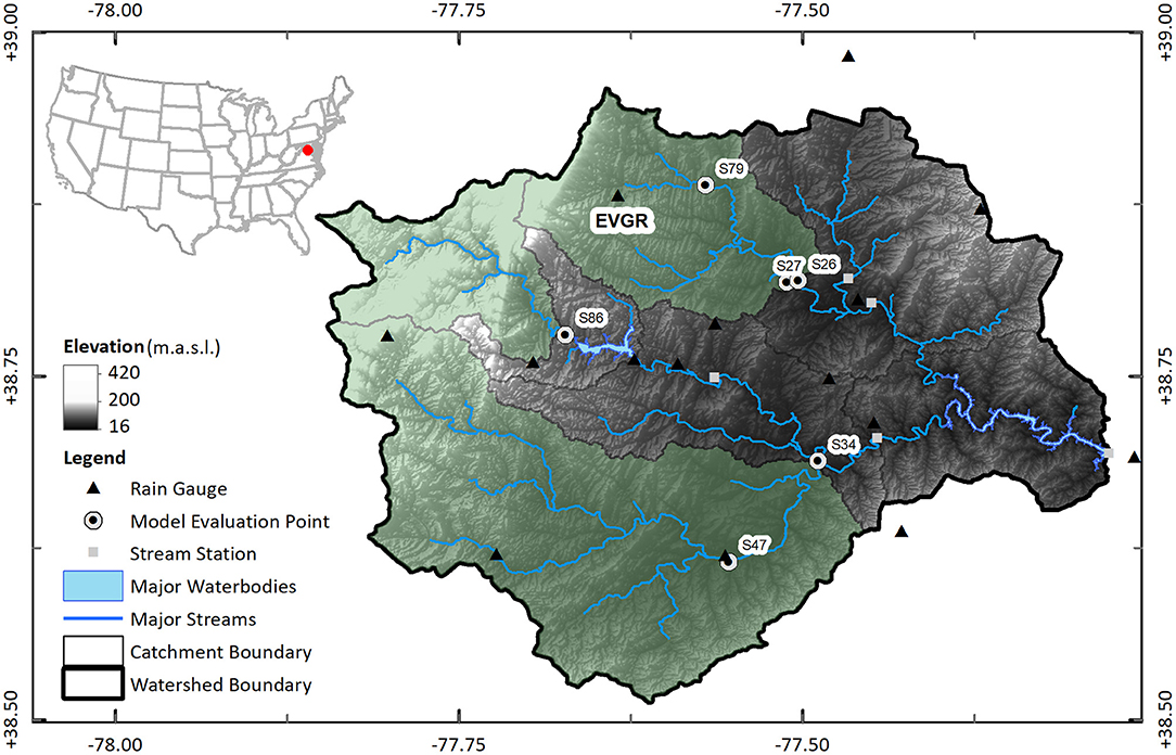
Figure 1. Study area showing the Occoquan Watershed boundary, 7 catchments, topography, major streams, major waterbodies, locations of rain gauges, and stream monitoring stations, and the locations of model evaluation points (S47, S86, and S79 coincide with stream monitoring stations).

Hydrologic Model

The Occoquan Watershed is modeled using the U.S. Environmental Protection Agency's (EPA) Hydrologic Simulation Program FORTRAN (HSPF). HSPF is a lumped-parameter continuous hydrologic and water quality model used to simulate the hydrology, streamflow and water quality of the watershed from there (3) components of a watershed: (1) pervious land areas, (2) impervious land aeras, and (3) well-mixed streams and reservoirs. The Occoquan Watershed HSPF model simulates various hydrological processes and associated water quality components in the watershed (Xu, 2005; Xu et al., 2007) in 5-year increments using precipitation observations, in-situ meteorological data and land use/cover. The Occoquan Watershed model is used to simulate streamflow (Q) and water quality indicators including stream temperature (TW), concentrations of total suspended solids (TSS), orthophosphate phosphorus (OP), total phosphorus (TP), ammonium-nitrate (NH₄-N), nitrate-nitrogen (NO₃-N), dissolved oxygen (DO), and biochemical oxygen demand (BOD) at six evaluation points (Figure 1) within the three catchments.

Q is simulated in HSPF using a built-in algorithm computing runoff, interflow, and groundwater. Runoff is estimated using the SCS Curve Number Method which computes surface runoff from contributing land areas. The runoff algorithm accounts for the fluxes and storages of water movement from rain, snow conditions, soil moisture, evapotranspiration, and infiltration capacity, simulated from land segments based on land cover, imperviousness, soil type, and topography while interflow is estimated assuming a liner relationship to storage. Q is simulated using a built-in hydraulic model function to simulate the hydraulic behavior in streams using storage-volume relationships, precipitation, and evaporation (Xu et al., 2007). TSS is a measurement of all suspended solids, both organic and inorganic, in a liquid, defined as solids larger than 0.7 mm whereas anything smaller is considered a dissolved solid. TSS is a visible and quantifiable indicator of overall water quality and a good representation of the sedimentation rate of a watershed. Concentrations of TSS is simulated in the HSPF model based on the production and removal of sediment from a contributing land segment. The algorithms representing land surface erosion in the HSPF model are derived from several older models based on the Modified Universal Soil Loss Equation from individual precipitation events. In-stream transport capacity of TSS is modeled using a built-in algorithm based on the modified form of the Stream Power Equation (Xu, 2005). Stream temperature is computed from the heat content of land surface runoff using the hear budget method to estimate the net heat exchange at the water surface from six heat components: shortwave solar radiation, longwave radiation, conduction-convection, evaporate heat loss, heat content of precipitation, and bed conditions (Xu, 2005). HSPF assumes that streams are unidirectional and well-mixed, thus thermal stratification is not considered in the model. DO and BOD are important indicators determining the overall health and quality of a waterbody to support life. DO is a measurement of gaseous oxygen dissolved in an aqueous solution, whereas BOD is a measurement of the amount of DO needed by aerobic organisms to break down organic matter. The in-stream DO concentration is estimated from surface runoff, computed as a direct function of water temperature, and from DO concentrations in interflow and active groundwater flows based on the processes of reaeration, decay of organic matter and benthal oxygen, and to a lesser degree, the estimated nitrification and photosynthesis rates applied to open water in HSPF (Xu, 2005). Potential BOD is estimated in HSPF using a built-in equation based on the conversion of biomass to BOD. Nitrogen-based nutrients, NH₄-N, and NO₃-N, are good indicators of water quality and, like their phosphorous-based counterpart, play a role in eutrophication, oxygen depletion, and biomass production. NH₄-N, or ammonium-nitrogen, is found in runoff from lawn care fertilizer or as a result of industrial and wastewater discharge. NO₃-N, or nitrate-nitrogen, is the concentration of nitrogen due to nitrates in waterbody. Phosphorus in aquatic systems is found in both soluble and insoluble forms. Insoluble phosphorous concentrations are related to the total sediment yield while the soluble nutrients account for the contribution from rainfall, land use, and anthropogenic impacts. TP is a measurement of all forms of phosphorus including OP, soluble phosphate-phosphorus, and organic phosphorus. Phosphorous is a limiting nutrient in the Occoquan watershed, which can play a role in the eutrophication, oxygen depletion, and biomass production if concentrations exceed need. In the Occoquan Watershed HSPF model, empirical relationships are built in between TP and sediment loads to simulate P concentrations in reaches, however, the spatial and temporal distribution of P is a limitation, as with most water quality models. To overcome this limitation, the Occoquan Watershed model is modeled with 87 unique segments to represent the temporal and spatial conditions of the watershed. HSPF uses a parent routine to simulate constituents involved in biological transformations, including total organic nitrogen (comprising of NH₄-N and NO₃-N), TP and OP. Equations are based on the components dependent on velocity of water in streams, the average depth of water, a set scouring factor, biomass concentrations, BOD concentrations, and a conversion rate from biomass to the respective constituent.

The model is composed of seven separate HSPF models, representing seven distinct catchments, linked together to create the overall watershed model. Three of the catchments (Upper Bull Run, Upper Broad Run, and Cedar Run), represented in Figure 1 in green, are the focus of this study. These three catchments are chosen since they represent the headwaters of the watershed prior to entering a major waterbody and are each monitored by a steam monitoring station near the confluence of the catchment.

The model is comprised of 87 land segments delineated within the seven catchments. The watershed delineation and segmentation process was originally performed in 2005 (Xu, 2005) using EPA's Better Assessment Science Integrating Point and Non-point sources (BASINS) software. Modeled segment delineations have undergone under several iterations to date and are comprised of discrete land areas based on geographic and physical characteristics of the watershed including topography, geography, land use, soil properties, and site features. Input into the model is at the segment level in hourly increments, which includes land use information and in-situ meteorological data. Land use is classified into 14 land use categories based on impervious coverage and soil properties. Meteorological data include precipitation, air temperature, cloud cover, dew point temperature, wind speed, solar radiation, and potential evapotranspiration. All meteorological data aside from precipitation are measured at one weather station operated by National Oceanic and Atmospheric Administration (NOAA) at the Washington Dulles International Airport, ~27 km from the centroid of the Occoquan Watershed. Data retrieved from the weather station are applied to the model as one uniform input to the entire watershed for those parameters in hourly increments. Precipitation is measured and inputted for each segment using a network of rain gauges within or proximate to the watershed. For this study, land use data and all meteorological data (i.e., air temperature, cloud cover, dew point temperature, wind speed, solar radiation, and potential evapotranspiration), aside from precipitation, are unaltered during model simulations. The only modification between model simulations is the precipitation input from four sources: rain gauge network (reference) and three SPPs (further discussed in section Data Sets).

Three of the six model evaluation points (S47, S79, and S86) are equipped with stream monitoring stations that are used in the calibration and validation of the hydrologic and water quality components of the model. These six model evaluation points vary in size and capture runoff from a number of segments, multiple rain gauges, and are represented by diverse land use and topographic conditions (Table 1).

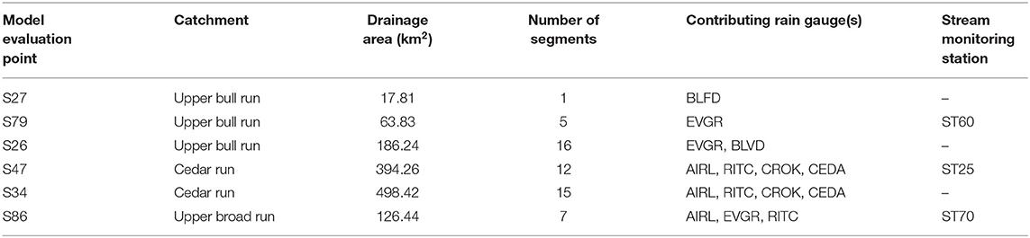
Table 1. Occoquan Watershed characteristics used in the HSPF model.

The HSPF model is calibrated (2008–2009) and validated (2010–2012) within a five-year period from January 1, 2008 to December 31, 2012 between rain gauge-simulated results and observed data obtained from eight stream monitoring stations located throughout the watershed. Each HSPF catchment model is calibrated prior to linking to the adjoining downstream HSPF catchment model. Calibration is performed on both daily and monthly streamflow and monthly loads of several water quality indicators. While model input is at the hourly scale, model output is at the daily scale to minimize timing errors commonly found using lower increment scales especially associated with over/under-predicting peaks and timing of event starts/stops. For detailed information regarding model setup, calibration, and performance, we refer the reader to Xu et al. (2007) and Solakian et al. (2019).

HSPF has been a long-standing, widely adopted hydrologic, and water quality model for its ability to simulate complex watersheds with various fate and transport processes within numerous land cover and climatic conditions (Albek et al., 2004; Mishra et al., 2007; Duda et al., 2012; Li et al., 2015; and others). While numerous past studies show satisfactory performance of simulated streamflow and water quality processes when evaluated on a continuous basis, the accuracy of HSPF-modeled concentration transport predictions shows to be (1) influenced by storm magnitude and frequency, (2) limited by the inability of ground-based meteorological stations to adequately cover the spatial extents and density necessary to represent watershed precipitation, and (3) seasonally dependent (Hayashi et al., 2004; Huo et al., 2015; Li et al., 2015; Stern et al., 2016). A few studies (Young et al., 2000; Wu et al., 2006; Diaz-Ramirez et al., 2013; and others) evaluated the propagation of errors in an HSPF model from input to output sugging that streamflow uncertainty is significantly impacted by precipitation patterns and magnitude, but may also be impacted by several other parameters and variables (e.g., land use classification, slope, infiltration capacity, soil moisture, groundwater recharge, and interflow recession) (Diaz-Ramirez et al., 2013). Additionally, Young et al. (2000) noted that the uncertainty associated with sediment transport loads and water quality constituents are greatly impacted by the quality of precipitation input. Within the Occoquan Watershed Model, the propagation of error from input precipitation to Q, TW, TSS, and DO simulated on a continuous basis over the 5-year study period show mixed performance. Overall, there appears to be dampening effect on SPP-simulated Q, TW and DO systematic error, however, error is amplified with SPP-simulated TSS. As mentioned, the Occoquan Watershed model is calibrated and validated on a continuous basis over a 5-year period which synthesizes the hydrologic process over a long period of hydroclimatic conditions, rather than event-based calibration which evaluates discrete rainfall-runoff events in isolation. It is acknowledged that continuous-based model calibration may have an impact on the accuracy of event-based simulation evaluations; however, since precipitation input is the only input parameter being altered in this analysis, a negligible impact on model performance is expected based on previous studies evaluating continuous versus event-based modeling (Ahn and Kim, 2016; Qiu et al., 2018; Xie et al., 2019a,b).

Data Sets

Four sets of precipitation data are evaluated in this study, namely the Occoquan Watershed rain gauge network and three SPPs: (1) the National Aeronautics and Space Administration (NASA) Tropical Rainfall Measuring Mission (TRMM) Multi-satellite Precipitation Analysis (TMPA) (Huffman et al., 2010); (2) the U.S. National Oceanic Atmospheric Administration (NOAA) Climate Prediction Center's (CPC) morphing technique (CMORPH) (Joyce et al., 2004); and (3) the Precipitation Estimation from Remotely Sensed Information using Artificial Neural Networks (PERSIANN)-Cloud Classification System (CCS) (Hsu et al., 2010). Precipitation data used as reference observations are obtained from a network of 15 tipping bucket rain gauges located within or proximate to the Occoquan Watershed, depicted in Figure 1 as black triangles. Gauges measure precipitation in increments of 0.254 mm (0.01 in.) by recording the time of occurrence of successive tips in hourly intervals throughout the span of this 5-year study (2008–2012). The recorded hourly precipitation is used as input for each segment in the Occoquan Watershed model from the nearest-neighbor rain gauge. Any missing precipitation data are interpolated for discrete hourly values using the infilling strategy outlined by Xu (2005).

The three quasi-global SPPs used in this study estimate precipitation using different algorithm and have different spatial and temporal resolutions, as outlined in Table 2. TMPA uses a combination of microwave and infrared sensors between 50°N and 50°S. This study uses the latent-calibrated, bias-adjusted TMPA 3B42-V7 product with a spatial resolution of 0.25° and a temporal resolution of 3 h (Huffman et al., 2007, 2010). The CMORPH product estimates precipitation derived from low orbit satellite passive microwave measurements transported via spatial propagation information obtained from geostationary satellites. CMORPH V1.0, used in this study, is bias corrected by matching raw data with the CPC daily gauge analysis over land and is available at a spatial and temporal resolution of 0.07° at equator and 0.5 h, respectively, between 60°N and 60°S (Joyce et al., 2004). PERSIANN-CCS, hereafter referred to as PERSIANN, is an infrared brightness temperature-based algorithm that extracts cloud features from geostationary satellites (Hsu et al., 1997, 2010; Sorooshian et al., 2000). The PERSIANN product uses gauge-corrected radar hourly data to calibrate cloud-top brightness temperature (Hong et al., 2007). PERSIANN is available at a spatial resolution of 0.04° and a temporal resolution of 0.5 h. Missing meteorological data for TMPA, CMORPH, and PERSIANN are estimated by temporally and spatially interpolating missing records. Each of the three SPPs are bias corrected based on weather radars and ground gauges, which may potentially include the Occoquan Watershed rain gauge network, making the reference not completely independent. Nevertheless, the intent of this study is to assess the relative performance of SPPs in simulating the hydrologic response of a watershed. Thus, the implication of having a few gauges used for bias correcting those products is considered minimal.

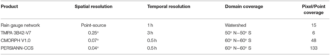
Table 2. Summary of the characteristics of precipitation data used in this study.

While precipitation data retrieved from rain gauges are inputted from a single source (the nearest-neighbor gauge), SPPs are areal-weighted and segment-aggregated (AWSA) spatially and temporally for each individual segment. Since each SPP is provided in a different temporal resolution, all data are matched to the hourly temporal scale. SPPs are also processed by spatially averaging precipitation estimates from pixels falling within the boundaries of each segment. For a detailed explanation of the precipitation infilling strategy and data processing employed in this study we refer the reader to Solakian et al. (2019). Hourly AWSA precipitation data are used as input in the HSPF model.

Event Selection

Eight extreme hydrometeorological events are evaluated in this study. These events are chosen according to the 95th percentile (R95p) of daily precipitation recorded by rain gauges over the 5-year study period. Precipitation events recorded at rain gauges in hourly increments were compiled into daily values and evaluated based on daily precipitation intensity (mm/d). Precipitation days with the highest intensity values were examined to confirm a representative storm across the watershed and then the R95p events were selected based on intensity values from one representative rain gauge (EVGR). To determine R95p events, an empirical cumulative density function (CDF) of maximum daily intensity (mm/d) derived from rain gauge observations is evaluated over the 5-year study period (Figure 2). Precipitation events are then grouped according to the maximum daily intensity 95th percentile, as discussed in section Results and Discussion. Event durations span from 24 to 120 h. Seven of the eight events in this study occur in spring (March–May) and fall (September–November), the other event, Event 8, is characterized as a convective storm during a period of unseasonably warm weather in December.

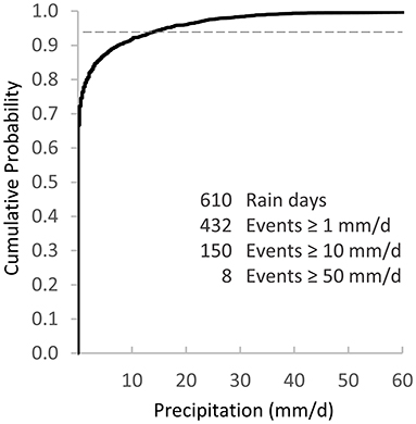
Figure 2. Cumulative density plot of daily precipitation and the number of precipitation events at representative rain gauge EVGR over the 5-year study period.

Table 3 presents the characteristics of selected hydrometeorological events. The total average accumulation is the average amount of rainfall accumulated (mm) at all six gauges over the duration of the event. Maximum daily intensity (mm/d) is the greatest daily rainfall amount accumulated over 1 day during the event. Events 4, 7, and 8 have a maximum daily intensity (mm/d) greater than the average accumulation over the duration of the event. Events 7 and 8 have a duration of 24 h, therefore the maximum daily intensity represents the event duration. For Event 4, a 96-h event, the maximum daily intensity is higher than the average event accumulation due to the disproportional spatial distribution of rainfall over the rain gauge network, where one gauge measured a higher value during a 1-day period, comparatively. Maximum hourly intensity (mm/h) is the largest rain rate over a 1-h period during the event recorded at a gauge.

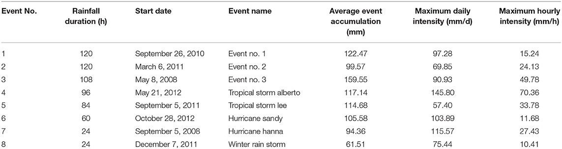
Table 3. Characteristics of selected hydrometeorological events.

Statistical Metrics

First, to analyze the performance of SPPs in comparison to gauge precipitation observations during extreme events, each SPP pixel overlaying a representative rain gauge location (e.g., pixel-to-point) is compared. Precipitation performance is evaluated based on average event accumulation (mm), mean precipitation (mm), and maximum hourly intensity (mm/h) for each of the eight extreme hydrometeorological events, as discussed in section Extreme Hydrometeorological Events. The average accumulation is the amount of total rainfall accumulated (mm) over the duration of the event. This amount represents the average accumulation over the six rain gauge locations, with σ being the standard deviation of measurements from the six locations. Mean precipitation is defined as the total accumulation divided by the duration in time of the event (mm/duration). Maximum hourly intensity (mm/h) is the greatest rainfall experienced at a rain gauge during the event over a 1-h period.

Second, the HSPF model is forced with the three SPPs to simulate output of streamflow and water quality indicators using processed AWSA precipitation input. Model output are evaluated at six evaluation points by comparing the three SPP-forced simulations to that forced with rain gauge-based records for each of the eight hydrometeorological events. The mean relative error of peak streamflow (E_p) is evaluated between SPP- and gauge-simulated streamflow (Equation 2) for each of the eight events. E_p is defined by Equation 1 as:

where Q_g is the peak gauge-simulated and Q_s is the peak SPP-simulated streamflow value (m³/s) over the duration of the event.

The performance of simulated model output including streamflow and water quality indicators are then comparatively evaluated using the following verification metrics: correlation coefficient (CC), relative bias (rB), and relative root mean-square error (rRMSE). CC is a measure of the linear argument between gauge-simulated and SPP-simulated output over the reference period with a perfect value of 1. rB is defined by Equation 2 as the difference between the gauge-simulated and SPP-simulated output, normalized by the gauge-simulated value (in %). Positive (negative) values indicate SPP-simulated output overestimation (underestimation), with a perfect value of 0%.

where Q_gi is the ith gauge-simulated and Q_si is the ith SPP-simulated streamflow/water quality indicator value. n is the total number of corresponding measurements.

rRMSE is a measure of random error, quantifying the error between the SPP-simulated output and the gauge-simulated output with a perfect value of 0%. rRMSE is defined by Equation 3 as follows:

Results and Discussion

Extreme Hydrometeorological Events

TMPA, CMORPH, and PERSIANN products are evaluated against gauge-based records for the eight extreme hydrometeorological events described in Table 3. These eight events range in duration from 24 to 120 h. Figure 3A shows the average event accumulation (mm), Figure 3B shows the mean precipitation (mm/duration), and Figure 3C shows the maximum hourly intensity (mm/h) measured from rain gauges, TMPA, CMORPH, and PERSIANN for the eight events. In general, longer events (i.e., Events 1 and 3) present a higher accumulation than shorter events (Events 7 and 8) although there are a few clear exceptions. For instance, the total accumulation of Event 6 (60 h) measured by the gauges, TMPA, and CMORPH is greater than Event 2 (120 h). Additionally, the total accumulation measured by the gauges for Events 4 and 5 is greater than Event 2. The variation around the mean accumulation (σ) at the six locations varies not only by product, but also by event. Gauge-based measurements have the greatest σ amongst all of the products, which is attributed to the nature (point) of the measurement. Interestingly, both TMPA and CMORPH tend to overestimate event-based rainfall accumulation for Event 1 and Event 3 (CMORPH only) and underestimate accumulation during shorter-duration events (Events 5, 7, and 8), whereas PERSIANN consistently underestimates total event accumulation for all events. Mean precipitation is inversely proportional to the event duration (Figure 3B). This is due to the fact that longer duration events (Events 1–3) are characterized by a mix of intermittent heavy and stratiform precipitation, whereas shorter events are typically of higher intensity. The same trend is noted for event accumulation, with PERSIANN grossly underestimating values (which is expected since mean precipitation is based on event accumulation). These results may be attributed to the fact that PERSIANN is based on a thermal infrared (IR) algorithm which has a tendency of missing light stratiform precipitation (Hong et al., 2007; Maggioni and Massari, 2018). Ebert et al. (2007) reported that in temperate climates IR-based SPPs generally are better able to detect heavy precipitation during warm season convective storms and decline in accuracy with stratiform precipitation. On the other hand, low orbiting passive microwave (PMW) satellite-based algorithms, such as TMPA and CMORPH, are known to underestimate heavy precipitation events associated with convective storms which is attributed to (1) the lack of fine temporal and spatial resolutions, which may make it difficult to track changes in short-term extreme events; (2) PMW sensor signal attenuation and non-uniform beam filling effects; and (3) bias corrections using gauge values undergoing interpolation that are known to smooth the extreme values (Qin et al., 2014; Oliveira et al., 2015) To support these claims, probability density functions (PDFs) of each precipitation product as a function of precipitation intensity (mm/hr) is provided in Figure 4 for one representative location (gauge EVGR). Hourly intensity is classified based on hourly intensity categories from the American Metrological Society. The PDFs reveal that all three SPPs have a tendency to detect more light precipitation (<2.5 mm) than recorded by the gauge. Furthermore, both TMPA and CMORPH generally tend to detect a larger number of moderate (2.5–7.5 mm) and heavy (>7.5 mm) intensity periods than PERSIANN (Events 1, 2, 3, 6, and 7) even though PERSIANN generally detects a higher hourly intensity (mm/h). These results show that while PERSIANN is better able to measure high intensity, the lower number of moderate and heavy intensity events recorded by PERSIANN actually reduces the total accumulation when compared to TMPA and CMORPH.

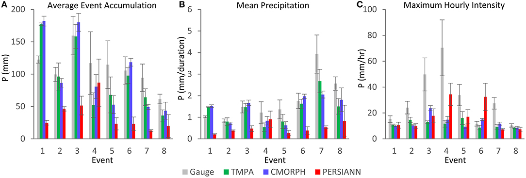
Figure 3. (A) Average event accumulation (mm), (B) mean precipitation (mm/duration), and (C) maximum hourly intensity (mm/h) for rain gauges, TMPA, CMORPH, and PERSIANN for eight extreme hydrometeorological events. The standard deviation of measurements across the study area is shown with gray error bars.

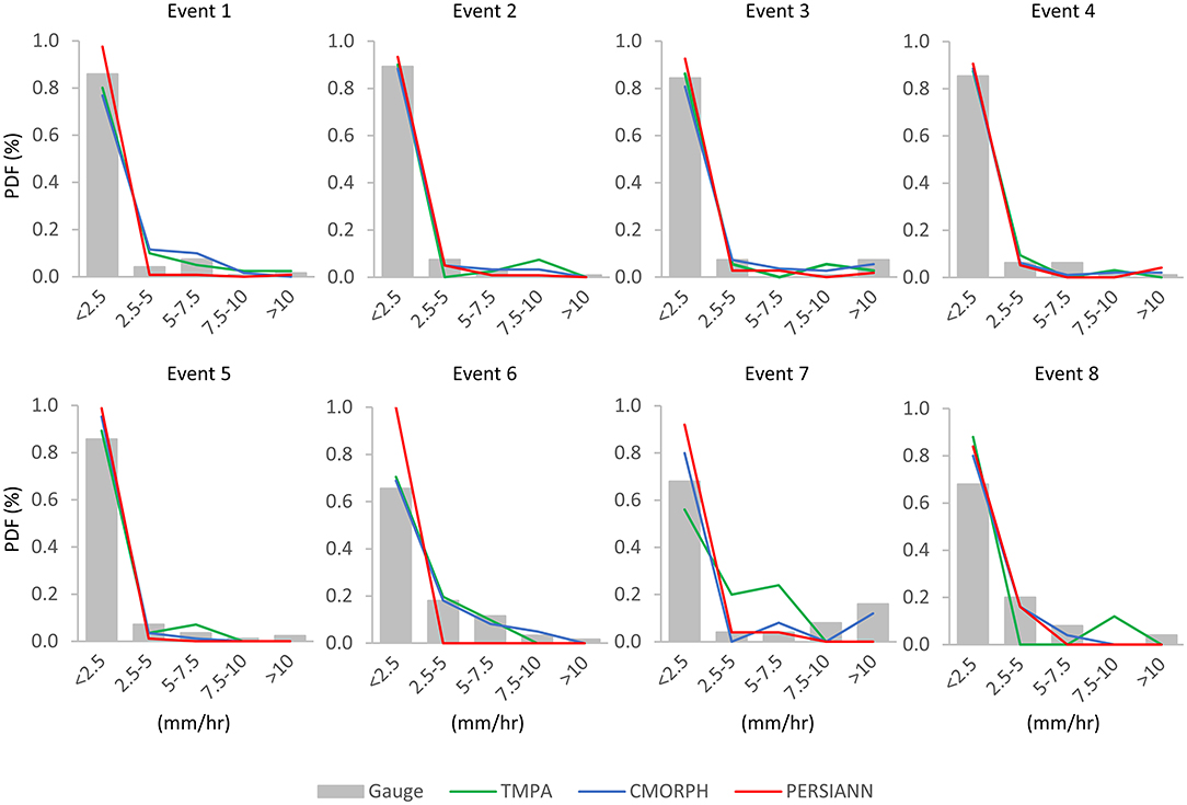
Figure 4. Probability Density Functions of events as a function of hourly intensity (mm/h) recorded at rain gauge EVGR, and by TMPA, CMORPH, and PERSIANN at gauge location EVGR during the eight hydrometeorological extreme events.

Maximum hourly intensity illustrates the dissimilarity of each product in the ability to measure heavy precipitation. Aside from one event (Event 6), gauge measurements far exceed all SPPs. However, PERSIANN, with a few exceptions, tends to better detect heavy precipitation in comparison to TMPA and CMORPH. The standard deviations of maximum hourly intensity, especially for Events 3 and 4, are significantly higher than other products indicating the variability of rainfall detected at different gauge locations. To highlight the variability of precipitation measurement throughout the watershed, Figure 5 presents the spatial characteristics of recorded maximum hourly intensity by the gauges (colored dots) and three SPPs (colored pixels) for Event 4, which has the highest standard deviation of precipitation recorded by the representative rain gauges.

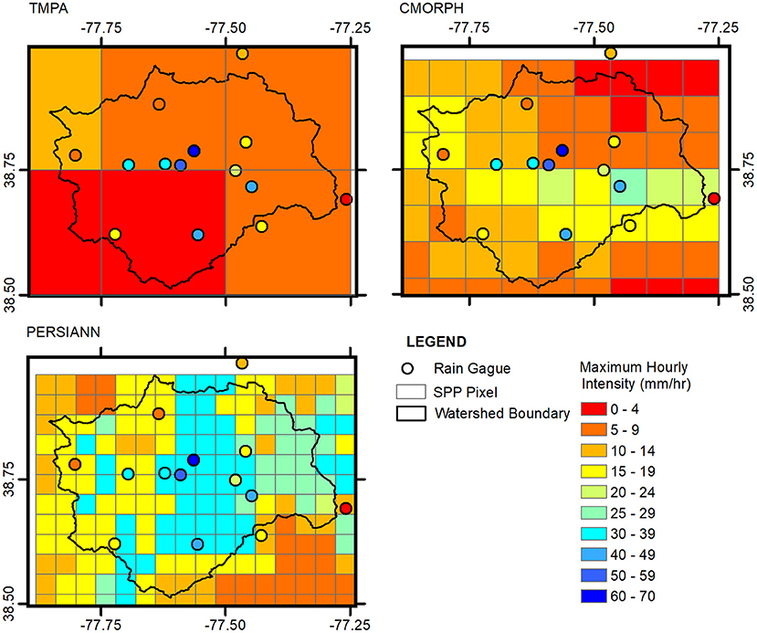
Figure 5. Spatial maps of maximum hourly intensity (mm/h) across the watershed as recorded by rain gauges, TMPA, CMORPH, and PERSIANN for Event 4.

Extreme-Event Simulated Streamflow

The capability of SPPs to simulate streamflow during extreme hydrometeorological events is evaluated by investigating the time series of hourly precipitation intensity (Figure 6) and hyetographs- hydrograph plots for each event (Figure 7). Overall, in terms of observed precipitation and gauge-simulated streamflow, TMPA and CMORPH simulations tend to well-capture the magnitude and timing of the peak events, however, there are a few exceptions. For Event 1, both TMPA and CMORPH grossly overestimate peak streamflow but are able to appropriately predict the timing of the peak. PERSIANN completely misses the streamflow peak in magnitude and timing resulting from its inability to accurately capture the accumulation of rainfall from intermittent stratiform precipitation between heavy intensity measurements during Event 1 which is seen in the hourly precipitation intensity. For Event 2, TMPA and CMORPH capture both the timing and peak magnitude of streamflow, though gauge-based streamflow presented a second but smaller peak that is largely undetected by both TMPA and CMORPH. Based on hourly precipitation intensity estimates during Event 2, TMPA and CMORPH captured rainfall intensity at the beginning of the event, however, did not well-capture rainfall during the second precipitation occurrence, thus leading to an underestimation of the second peak. Similar results are found with Events 3, 5, and 6 where TMPA and CMORPH are able to capture the peak magnitude of streamflow, though timing is delayed for Events 3 and 5.

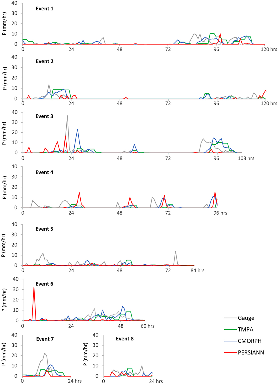
Figure 6. Precipitation time series plots of hourly intensity (mm/h) recorded at rain gauge EVGR, and by TMPA, CMORPH, and PERSIANN at gauge location EVGR during the eight hydrometeorological extreme events.

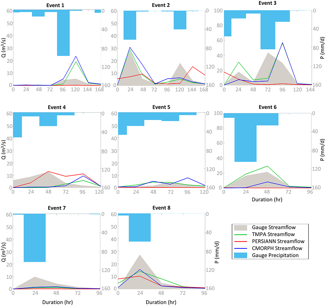
Figure 7. Hyetograph of the eight hydrological extreme events based on observations of daily precipitation intensity (mm/day) at gauge EVGR and corresponding hydrographs of modeled streamflow (m³/s) for gauge-, TMPA-, CMORPH-, and PERSIANN-simulated data at evaluation point S79.

PERSIANN exhibited the best performance for Event 4, able to capture the peak magnitude and timing of streamflow. During Event 4, PERSIANN captures the intermittent intense precipitation over the duration of the event, whereas TMPA, and to a lesser degree CMORPH, cannot match hourly intensities observed from gauges early on in the event, and overestimate precipitation in later stages of the event's duration which is evident from the hourly precipitation intensity time series (Figure 6). All three SPPs are unable to capture precipitation intensity during Event 7 and thus significantly underpredict peak streamflow. Though Event 7 and Event 8 are classified as 24-h events, and the average event accumulation (mm) and daily intensity (mm/d) are higher for Event 7, the peak streamflow simulated for Event 8 is greater. This is mostly likely due to the seasonal performance built into the HSPF model. Event 8 occurs in December whereas Event 7 occurs in September. HSPF inherently generates greater runoff from the watershed from reduced infiltration rates during cooler months (December–March), thus produces higher simulated streamflow than in warmer seasons.

To quantify the error associated with the peak magnitude of streamflow for each event, E_p is determined and averaged among all six evaluation points. Figure 8 displays the mean error of peak SPP-simulated streamflow in comparison to gauge-simulated streamflow. The most significant error in peak is associated with Event 1 where both TMPA and CMORPH significantly overestimate the peak magnitude at several evaluation points. The overestimation of the peak magnitude streamflow results from TMPA and CMORPH both estimating a higher precipitation accumulation during Event 1 than observed at the rain gauges. Except for Event 4, PERSIANN tends to underestimate peak magnitude of streamflow for all events. Aside from Event 6, results from TMPA and CMORPH are fairly consistent which is expected since they are based on similar input satellite retrievals to estimate precipitation. The inconsistency in peak magnitude of streamflow between TMPA and CMORPH for Event 6 is attributed to the temporal resolution of the two products, 3 and 0.5 h, respectively. In the 3-h window of TMPA, the duration of precipitation intensity is overestimated for TMPA when compared to CMORPH which then resulted in a higher simulated peak magnitude streamflow.

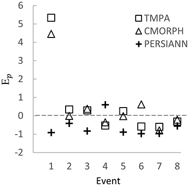
Figure 8. Mean peak streamflow error of TMPA, CMORPH, and PERSIANN with respect to gauge-simulated streamflow.

Streamflow and Water Quality Error Analysis

To assess model performance in simulating streamflow and water quality indicators between gauge-simulated output and SPP-simulated output, three error metrics are used: CC, rB, and rRMSE. Error is measured at the daily timestep and evaluated at six evaluation points over the duration of the defined event for Q, TW, and concentrations of TSS, DO, BOD, and nutrients OP, TP, NH₄-N, NO₃-N. Results indicate fairly good agreement (Figure 9) between gauge- and SPP-simulated Q for TMPA and CMORPH (CCs between 0.8 and 1.0 with a mean CC of 0.81 and 0.86 representative of all events, respectively) aside from Event 4, which is missed by all SPPs. The CC of PERSIANN-simulated Q is generally lowest among SPPs (mean CC of 0.64), due to its inability to accurately measure stratiform precipitation between intense periods of precipitation during an event. rB (Figure 10) varies significantly for Q indicating SPPs either under- (negative) or over- (positive) predict Q. Highest rB errors for TMPA and CMORPH are 225 and 150%, respectively, and −100% for PERSIANN which all occur with Event 1. Events 2 and 5 have good agreement between gauge- and SPP-simulated Q. rRMSEs are somewhat consistent between SPPs for each event (Figure 11), however, high rRMSEs for TMPA and CMORPH are noted for Event 1, whereas the rRMSE of PERSIANN is fairly consistent between events. The high rRMSE values associated with Event 1 for TMPA and CMORPH are likely due the SPP's ability, as a gridded product with larger spatial resolution, to pick up localized precipitation, where some rain gauges did not record the same precipitation intensity during the event.

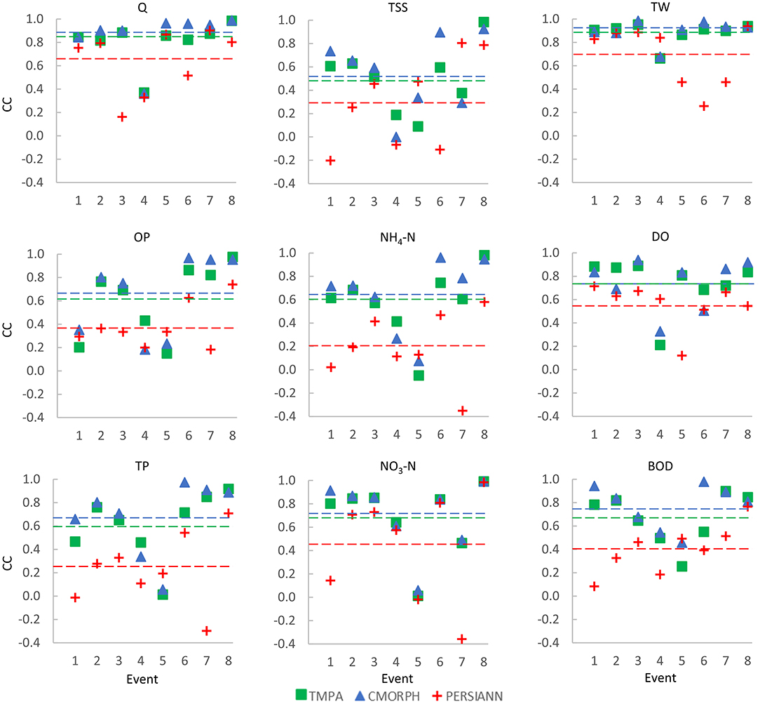
Figure 9. Correlation coefficients of streamflow and water quality indicators between gauge-simulated and SPP-simulated output for TMPA, CMORPH, and PERSIANN for six evaluation points. The mean indicator value across all eight events is represented by a dashed line corresponding to TMPA, CMORPH, and PERSIANN in green, blue, and red, respectively.

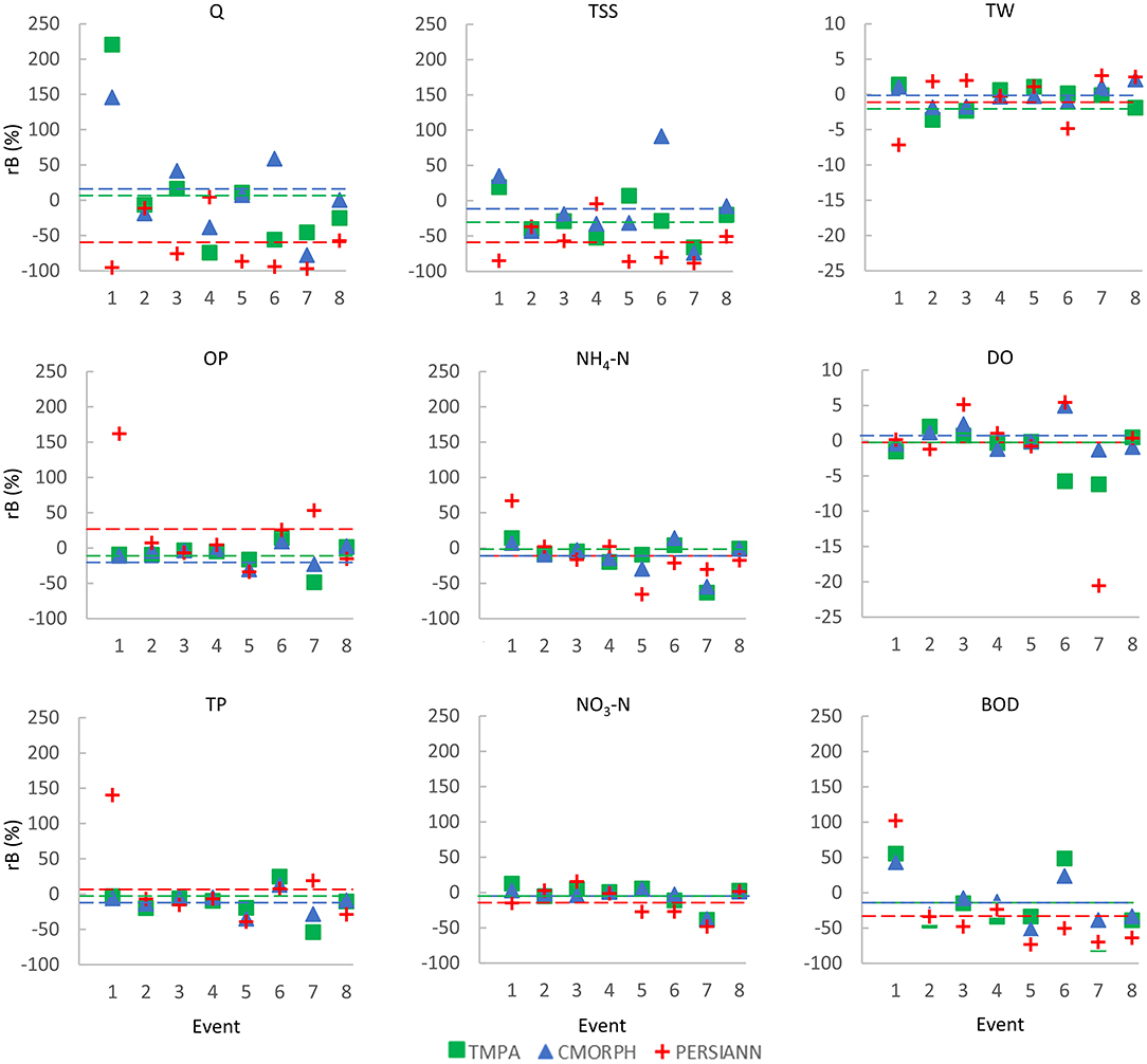
Figure 10. rBs of streamflow and water quality indicators between gauge-simulated and SPP-simulated output for TMPA, CMORPH, and PERSIANN for six evaluation points. The mean indicator value across all eight events is represented by a dashed line corresponding to TMPA, CMORPH, and PERSIANN in green, blue, and red, respectively.

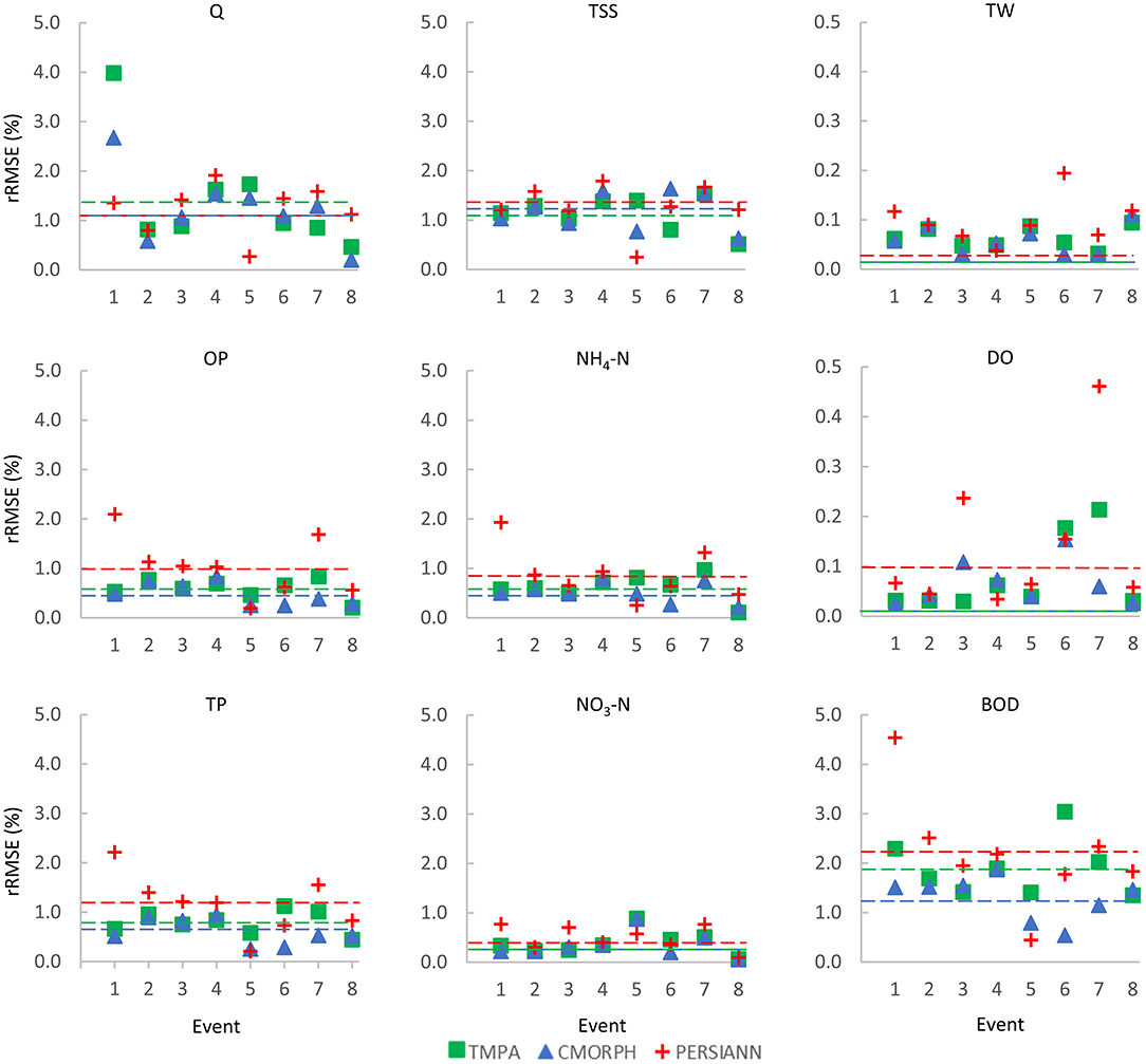
Figure 11. rRMSEs of streamflow and water quality indicators between gauge-simulated and SPP-simulated output for TMPA, CMORPH, and PERSIANN for six evaluation points. The mean indicator value across all eight events is represented by a dashed line corresponding to TMPA, CMORPH, and PERSIANN in green, blue, and red, respectively.

Correlations (Figure 9) of water quality indicators vary considerably, however, TW has the strongest positive linear relationship compared to other indicators evaluated in this study. Strong correlations are attributed to in-stream temperature being naturally dependent on ambient air temperature conditions with precipitation, and thus streamflow, having a lesser impact of TW. Correlations fall between 0.8 to 1.0 for TMPA and CMORPH for all events except for Event 4. PERSIANN-simulated TW shows weaker correlations, especially for Events 5, 6, and 7. Mean CC values representative of all events for TMPA, CMORPH, and PERSIANN are 0.88, 0.90, and 0.69, respectively. rB (Figure 10) and rRMSE (Figure 11) for TW are also lowest (better agreement) among all simulated output indicating that TW is more impacted by ambient air temperature than precipitation.

SPP-simulated TSS, a flow-dependent variable, has the weakest relationship to gauge-simulated TSS (Figure 9) for all water quality indicators, with CMORPH (mean CC of 0.55) performing slightly better than TMPA and considerably better than PERSIANN (mean CC of 0.50 and 0.30, respectively). PERSIANN presents negative correlations during Events 1, 4, and 6 and generally performs worse than both TMPA and CMORPH, aside from two events (Events 5 and 7). Event 5 is characterized by a multi-day duration and lower-intensity precipitation than other events evaluated in this study. While PERSIANN misses the magnitude of peak TSS, CMORPH and TMPA both overpredict it. Event 8 presents a high correlation, and low rB (Figure 10) and rRMSE (Figure 11) for SPP-simulated TSS indicating that all three SPPs well capture TSS concentrations, likely due to the short duration of the event (24 h) and the high skill of SPP-simulated Q, which directly influences TSS, especially during early stages of a storm event. In a study across the same watershed, Solakian et al. (2019) found a direct relationship between simulated streamflow and TSS concentrations, with peaks well-represented in both TMPA and CMORPH simulations; however, TSS concentrations tend to be low throughout warmer months aside from a few instances where intense precipitation is captured and translated into peak streamflow.

Correlations of DO between SPP- and gauge-simulations during a 5-year continuous period are 0.81–0.85 (Solakian et al., 2019) indicating good agreement on a continuous basis. Correlations of event-based simulations (Figure 9) of DO suggest that model skill varies by event with majority of correlations above 0.8 and a mean CC of 0.74 for both TMPA and CMORPH, with a few exceptions. PERSIANN exhibits overall inferior performance for simulated DO concentrations (mean CC of 0.56) aside from Event 4. Both TMPA and CMORPH missed the peak Q for Event 4 whereas PERSIANN was able to able to well-capture the timing and peak magnitude of Q, thus translating into a higher correlation of DO for Event 4 when compared to the other SPPs. Both rB (Figure 10) and rRMSE (Figure 10) for DO are much lower compared to other water quality indicators, with the exception of TW. The relatively small change in DO concentrations are probably not associated with precipitation. Rather DO is more temperature-dependent which is evident from seasonal fluctuations of DO concentrations. Correlations of BOD appear to mimic TSS, though rB and rRMSE of SPP-simulated BOD vary considerably. Mean CCs for TMPA, CMORPH, and PERSIANN, representative for all events, are 0.66, 0.77, and 0.40, respectively. CMORPH outperforms TMPA, and both CMORPH and TMPA significantly outperform PERSIANN aside from Event 5, where PERSIANN outperforms other SPPs. From a seasonal perspective, simulated BOD concentrations increase in warmer periods and drop during cooler periods following patterns associated with TW, yet this indicator also appears to be influenced by TSS concentrations during peak events.

Two phosphorus-based compartments of phosphorous are investigated in this study: TP and OP. The Occoquan Watershed model, built with precipitation input at 87 individual segments, is able to well-capture changes of simulated nutrient loads due to changes in precipitation input from the four data sources: rain gauges, TMPA, CMORPH, and PERSIANN. The behavior of TP and OP concentrations follow similar agreement between SPP- and gauge-simulations as with TSS, and have similar correlations (Figure 9). The mean CCs for TMPA, CMORPH, and PERSIANN for TP and OP are 0.60, 0.67, 0.23 and 0.61, 0.65, 0.38, respectively. rB of TP and OP are inversely proportional to TSS which may be due to the influence of both insoluble (sediment-dependent) and soluble (precipitation-dependent) forms of phosphorous included in the model (Figure 10). Overall, all three SPP-simulated TP and OP outputs are fairly consistent with no clear indication of one outperforming another. The one exception to consistence in performance is PERSIANN-simulated TP and OP (rB = +140% and +160%, respectively) for Event 1. These results suggest that, while TP and OP may be sediment-dependent indicators most likely tied to land use conditions in the watershed and the spatial and temporal differences in precipitation have a lesser impact on simulated TP and OP concentrations.

Nitrogen-based nutrients, NH₄-N, and NO₃-N, are investigated based on a comparison of SPP-simulated to gauge-simulated concentrations. SPP-simulated NH₄-N and NO₃-N present similar correlations to TSS with mean CCs of 0.57, 0.64, 0.20 and 0.68, 0.70, 0.45, respectively (Figure 9). Additionally, rB (Figure 10) and rRMSE (Figure 11) present consistent values, aside for rB values for NH₄-N for Event 1 which present an inverse relationship. SPP-simulated NO₃-N correlations, rBs, and rRMSEs present similar results among the three SPPs indicating that the spatial and temporal differences of SPPs have little impact on simulation skill.

Conclusions

Eight extreme events within the study period are identified according to the 95th percentile of daily precipitation recorded by rain gauges during the study period. Event durations span from 24 to 120 h. Event-based error is measured at the daily timestep and evaluated at six evaluation points for Q, TW, and concentrations of TSS, DO, BOD, and nutrients OP, TP, NH₄-N, NO₃-N. Results indicate fairly good agreement between gauge- and SPP-simulated Q for TMPA, whereas PERSIANN-simulated Q is generally lowest among SPPs, due to its inability to accurately measure stratiform precipitation between intense periods of precipitation during an event. The skill of SPP- to gauge-simulated water quality indicators vary considerably. However, TW has the strongest agreement compared to other indicators evaluated in this study. SPP-simulated TSS, a flow-dependent variable, has the weakest relationship to gauge-simulated TSS among all water quality indicators, with CMORPH performing slightly better than TMPA and PERSIANN. Strong agreement of TW simulations is attributed to in-stream temperature being naturally dependent on ambient air temperature conditions with precipitation, and thus streamflow, having a lesser impact. For both DO and BOD, event-based simulations suggest that model skill varies by event though SPP-simulated output shows overall good agreement to gauge-simulated output, with a few exceptions. PERSIANN exhibits overall inferior performance for simulated DO and BOD concentrations. For phosphorus-based nutrient simulations of TP and OP, all three SPP-simulated TP and OP outputs are fairly consistent with no clear indication of one outperforming another suggesting that while TP and OP may be sediment-dependent indicators most likely tied to land use conditions in the watershed and the spatial and temporal differences in precipitation have a low impact on simulated TP and OP concentrations. Nitrogen-based nutrients, NH₄-N, and NO₃-N, present similar results among the three SPPs indicating that the spatial and temporal differences of SPPs have less of an impact on simulation skill that other water quality indicators.

Overall, this study demonstrates that the spatiotemporal variability of SPPs, along with their different algorithms, are capable of predicting the characteristics of streamflow and water quality simulations with varying degrees of performance during hydrometeorological extreme events. However, there are limitations to this study. Foremost, the study area, suburban Washington, D.C., is situated in a region characterized by a temperate climate and mild topographic variation with moderate precipitation intensity. Both climate and topography may have a significant impact on SPP performance. Secondly, this analysis was conducted in a single location utilizing only one hydrology/water quality model, i.e., HSPF. While this model is well-calibrated and has been validated to observation results, another model may respond in a different way to changes in streamflow and water quality indicators resulting from forcing precipitation inputs especially during extreme hydrometeorological events. Additionally, the model was calibrated on a continuous basis over the study period whereas calibration based on only discrete events may produce different results. Thirdly, the model was calibrated based on rain gauge data, which may not reflect the actual distribution, extents, or magnitude of precipitation in the watershed. Lastly, while this study provides a comprehensive evaluation of three of the most widely used SPPs, TMPA, CMORPH, and PERSIANN, it does not consider an exhaustive list of precipitation sources such as other SPPs, blended and reanalysis products, or radar data which would likely present different results. Nonetheless, this work represents a novel approach to utilizing SPPs data for water quality modeling during extreme hydrometeorological events, which could be of beneficial in locations lacking ground-based instruments to measure precipitation. Future research should evaluate the applicability of SPPs for simulating water quality in different regions, climates and other hydrometeorological extremes such as droughts and long-term hydroclimatic changes. Additionally, different hydrology/water quality models may be used to simulate results as well as using other precipitation products such as re-analysis and blended products.

Data Availability Statement

The raw data supporting the conclusions of this article will be made available by the authors, without undue reservation.

Author Contributions

JS and VM designed the research objectives and developed the methods employed in this study. JS processed the data, carried out the analysis, and primarily authored the manuscript with contributions from VM and AG. VM provided guidance and oversaw the work and AG provided analysis and guidance on results and findings. All authors reviewed the draft manuscript and provided feedback.

Conflict of Interest

The authors declare that the research was conducted in the absence of any commercial or financial relationships that could be construed as a potential conflict of interest.

Acknowledgments

The authors thank Editor Giulia Sofia and the two reviewers for their suggestions constructive comments that improved this manuscript. The authors also want to thank Dr. Adnan Lodhi who developed and ran the Occoquan Watershed model used in this analysis. The authors would like to recognize the financial supporters of the Occoquan Watershed Monitoring Program and the Occoquan Watershed Model.

Supplementary Material

The Supplementary Material for this article can be found online at: https://www.frontiersin.org/articles/10.3389/fenvs.2020.585451/full#supplementary-material

References

AghaKouchak, A., Behrangi, A., Sorooshian, S., Hsu, K., and Amitai, E. (2011). Evaluation of satellite-retrieved extreme precipitation rates across the central United States. J. Geophys. Res. 116:D02115. doi: 10.1029/2010JD014741
Ahn, S.-R., and Kim, S.-J. (2016). The effect of rice straw mulching and no-tillage practice in upland crop areas on nonpoint-source pollution loads based on HSPF. Water 8:106. doi: 10.3390/w8030106
Albek, M., Bakir Ögütveren, Ü., and Albek, E. (2004). Hydrological modeling of Seydi Suyu watershed (Turkey) with HSPF. J. Hydrol. 285, 260–271. doi: 10.1016/j.jhydrol.2003.09.002
Alexander, L. V., Fowler, H. J., Bador, M., Behrangi, A., Donat, M. G., Dunn, R., et al. (2019). On the use of indices to study extreme precipitation on sub-daily and daily timescales. Environ. Res. Lett. 14:125008. doi: 10.1088/1748-9326/ab51b6
Bharti, V., Singh, C., Ettema, J., and Turkington, T. A. R. (2016). Spatiotemporal characteristics of extreme rainfall events over the Northwest Himalaya using satellite data: spatiotemporal characteristics of extreme rainfall events. Int. J. Climatol. 36, 3949–3962. doi: 10.1002/joc.4605
Chen, S., Liu, B., Tan, X., and Wu, Y. (2020). Inter-comparison of spatiotemporal features of precipitation extremes within six daily precipitation products. Clim. Dyn. 54, 1057–1076. doi: 10.1007/s00382-019-05045-z
Chintalapudi, S., Sharif, H., and Xie, H. (2014). Sensitivity of distributed hydrologic simulations to ground and satellite based rainfall products. Water 6, 1221–1245. doi: 10.3390/w6051221
de Oliveira, V. A., de Mello, C. R., Beskow, S., Viola, M. R., and Srinivasan, R. (2019). Modeling the effects of climate change on hydrology and sediment load in a headwater basin in the Brazilian Cerrado biome. Ecol. Eng. 133, 20–31. doi: 10.1016/j.ecoleng.2019.04.021
Demirdjian, L., Zhou, Y., and Huffman, G. J. (2018). Statistical modeling of extreme precipitation with TRMM data. J. Appl. Meteor. Climatol. 57, 15–30. doi: 10.1175/JAMC-D-17-0023.1
Derin, Y., Anagnostou, E., Berne, A., Borga, M., Boudevillain, B., Buytaert, W., et al. (2016). Multiregional satellite precipitation products evaluation over complex terrain. J. Hydrometeorol. 17, 1817–1836. doi: 10.1175/JHM-D-15-0197.1
Derin, Y., Nikolopoulos, E., and Anagnostou, E. N. (2019). “Chapter Seven -Estimating extreme precipitation using multiple satellite-based precipitation products,” in Extreme Hydroclimatic Events and Multivariate Hazards in a Changing Environment, eds. V. Maggioni and C. Massari (Cambridge, MA: Elsevier, Inc), 163–190.
Diaz-Ramirez, J., Johnson, B., McAnally, W., Martin, J., and Camacho, R. (2013). Estimation and propagation of parameter uncertainty in lumped hydrological models: a case study of HSPF model applied to luxapallila creek Watershed in Southeast USA. J. Hydrogeol. Hydrol. Eng. 2:1. doi: 10.4172/2325-9647.1000105
Duda, P., Hummel, P., Donigian, A. S. Jr, and Imhoff, A. C. (2012). BASINS/HSPF: model use, calibration, and validation. Trans. ASABE 55, 1523–1547. doi: 10.13031/2013.42261
Ebert, E. E., Janowiak, J. E., and Kidd, C. (2007). Comparison of near-real-time precipitation estimates from satellite observations and numerical models. Bull. Amer. Meteor. Soc. 88, 47–64. doi: 10.1175/BAMS-88-1-47
Gourley, J. J., Hong, Y., Flamig, Z. L., Wang, J., Vergara, H., and Anagnostou, E. N. (2011). Hydrologic evaluation of rainfall estimates from radar, satellite, gauge, and combinations on Ft. Cobb Basin, Oklahoma. J. Hydrometeor. 12, 973–988. doi: 10.1175/2011JHM1287.1
Habib, E., Henschke, A., and Adler, R. F. (2009). Evaluation of TMPA satellite-based research and real-time rainfall estimates during six tropical-related heavy rainfall events over Louisiana, USA. Atmosph. Res. 94, 373–388. doi: 10.1016/j.atmosres.2009.06.015
Hayashi, S., Murakami, S., Watanabe, M., and Bao-Hua, X. (2004). HSPF simulation of runoff and sediment loads in the upper Changjiang river basin, China. J. Environ. Eng. 130, 801–815. doi: 10.1061/(ASCE)0733-9372(2004)130:7(801)
Hazra, A., Maggioni, V., Houser, P., Antil, H., and Noonan, M. (2019). A Monte Carlo-based multi-objective optimization approach to merge different precipitation estimates for land surface modeling. J. Hydrol. 570, 454–462. doi: 10.1016/j.jhydrol.2018.12.039
Hong, Y., Gochis, D., Cheng, J., Hsu, K., and Sorooshian, S. (2007). Evaluation of PERSIANN-CCS rainfall measurement using the NAME Event Rain Gauge network. J. Hydrometeor. 8, 469–482. doi: 10.1175/JHM574.1
Hsu, K., Behrangi, A., Imam, B., and Sorooshian, S. (2010). “Extreme precipitation estimation using satellite-based PERSIANN-CCS algorithm,” in Satellite Rainfall Applications for Surface Hydrology, eds. M. Gebremichael, and F. Hossain (Dordrecht: Springer).
Hsu, K., Gao, X., Sorooshian, S., and Gupta, H. V. (1997). Precipitation estimation from remotely sensed information using artificial neural networks. J. Appl. Meteorol. 36, 1176–1190. doi: 10.1175/1520-0450(1997)036%3C1176:PEFRSI%3E2.0.CO;2
Huang, Y., Chen, S., Cao, Q., Hong, Y., Wu, B., Huang, M., et al. (2013). Evaluation of version-7 TRMM multi-satellite precipitation analysis product during the beijing extreme heavy rainfall event of 21 July 2012. Water 6, 32–44. doi: 10.3390/w6010032
Huffman, G. J., Bolvin, D. T., and Nelkin, E. J. (2010). “The TRMM Multi-Satellite Precipitation Analysis (TMPA),” in Satellite Rainfall Applications for Surface Hydrology, eds. M. Gebremichael and F. Hossain (Dordrecht: Springer), 3–22.
Huffman, G. J., Bolvin, D. T., Nelkin, E. J., Wolff, D. B., Adler, R. F., Gu, G., et al. (2007). The TRMM Multisatellite Precipitation Analysis (TMPA): quasi-global, multiyear, combined-sensor precipitation estimates at fine scales. J. Hydrometeor. 8, 38–55. doi: 10.1175/JHM560.1
Huo, S.-C., Lo, S.-L., Chiu, C.-H., Chiueh, P.-T., and Yang, C.-S. (2015). Assessing a fuzzy model and HSPF to supplement rainfall data for nonpoint source water quality in the Feitsui reservoir watershed. Environ. Model. Softw. 72, 110–116. doi: 10.1016/j.envsoft.2015.07.002
Jeznach, L. C., Hagemann, M., Park, M.-H., and Tobiason, J. E. (2017). Proactive modeling of water quality impacts of extreme precipitation events in a drinking water reservoir. J. Environ. Manag. 201, 241–251. doi: 10.1016/j.jenvman.2017.06.047
Jiang, S., Liu, S., Ren, L., Yong, B., Zhang, L., Wang, M., et al. (2018). Hydrologic evaluation of six high resolution satellite precipitation products in capturing extreme precipitation and streamflow over a medium-sized Basin in China. Water 10:25. doi: 10.3390/w10010025
Jiang, S., Zhang, Z., Huang, Y., Chen, X., and Chen, S. (2017). Evaluating the TRMM multisatellite precipitation analysis for extreme precipitation and streamflow in ganjiang river basin, China. Adv. Meteorol. 2017:2902493. doi: 10.1155/2017/2902493
Joyce, R. J., Janowiak, J. E., Arkin, P. A., and Xie, P. (2004). CMORPH: a method that produces global precipitation estimates from passive microwave and infrared data at high spatial and temporal resolution. J. Hydrometeorol. 5, 487–503. doi: 10.1175/1525-7541(2004)005<0487:CAMTPG>2.0.CO;2
Katiraie-Boroujerdy, P.-S., Ashouri, H., Hsu, K., and Sorooshian, S. (2017). Trends of precipitation extreme indices over a subtropical semi-arid area using PERSIANN-CDR. Theor. Appl. Climatol. 130, 249–260. doi: 10.1007/s00704-016-1884-9
Kubota, T., Ushio, T., Shige, S., Kida, S., Kachi, M., and Okamoto, K. (2009). Verification of high-resolution satellite-based rainfall estimates around japan using a gauge-calibrated ground-radar dataset. J. Meteorol. Soc. Japan 87A, 203–222. doi: 10.2151/jmsj.87A.203
Kwon, E.-H., Sohn, B.-J., Chang, D.-E., Ahn, M.-H., and Yang, S. (2008). Use of numerical forecasts for improving TMI rain retrievals over the mountainous area in Korea. J. Appl. Meteor. Climatol. 47, 1995–2007. doi: 10.1175/2007JAMC1857.1
Li, X., Zhang, Q., and Ye, X. (2013). Dry/wet conditions monitoring based on TRMM rainfall data and its reliability validation over Poyang Lake Basin, China. Water 5, 1848–1864. doi: 10.3390/w5041848
Li, Z., Liu, H., Luo, C., Li, Y., Li, H., Pan, J., et al. (2015). Simulation of runoff and nutrient export from a typical small watershed in China using the hydrological simulation program–Fortran. Environ. Sci. Pollut. Res. 22, 7954–7966. doi: 10.1007/s11356-014-3960-y
Lockhoff, M., Zolina, O., Simmer, C., and Schulz, J. (2014). Evaluation of satellite-retrieved extreme precipitation over europe using gauge observations. J. Clim. 27, 607–623. doi: 10.1175/JCLI-D-13-00194.1
Ma, D., Xu, Y.-P., Gu, H., Zhu, Q., Sun, Z., and Xuan, W. (2019). Role of satellite and reanalysis precipitation products in streamflow and sediment modeling over a typical alpine and gorge region in Southwest China. Sci. Total Environ. 685, 934–950. doi: 10.1016/j.scitotenv.2019.06.183
Maggioni, V., and Massari, C, (eds.). (2019). Extreme Hydroclimatic Events and Multivariate Hazards in a Changing Environment A Remote Sensing Approach, 1st Edn. Cambridge, MA: Elsevier, Inc.
Maggioni, V., and Massari, C. (2018). On the performance of satellite precipitation products in riverine flood modeling: a review. J. Hydrol. 558, 214–224. doi: 10.1016/j.jhydrol.2018.01.039
Maggioni, V., Nikolopoulos, E. I., Anagnostou, E. N., and Borga, M. (2017). Modeling satellite precipitation errors over mountainous terrain: the influence of gauge density, seasonality, and temporal resolution. IEEE Trans. Geosci. Remote Sensing 55, 4130–4140. doi: 10.1109/TGRS.2017.2688998
Maggioni, V., Vergara, H. J., Anagnostou, E. N., Gourley, J. J., Hong, Y., and Stampoulis, D. (2013). Investigating the applicability of error correction ensembles of satellite rainfall products in river flow simulations. J. Hydrometeor. 14, 1194–1211. doi: 10.1175/JHM-D-12-074.1
Mahbod, M., Shirvani, A., and Veronesi, F. (2019). A comparative analysis of the precipitation extremes obtained from tropical rainfall-measuring mission satellite and rain gauges datasets over a semiarid region. Int. J. Climatol. 39, 495–515. doi: 10.1002/joc.5824
Mehran, A., and AghaKouchak, A. (2014). Capabilities of satellite precipitation datasets to estimate heavy precipitation rates at different temporal accumulations: capabilities of satellite data to estimate heavy precipitation rates. Hydrol. Process. 28, 2262–2270. doi: 10.1002/hyp.9779
Mei, Y., Nikolopoulos, E., Anagnostou, E., Zoccatelli, D., and Borga, M. (2016). Error analysis of satellite precipitation-driven modeling of flood events in complex alpine terrain. Remote Sensing 8:293. doi: 10.3390/rs8040293
Meng, J., Li, L., Hao, Z., Wang, J., and Shao, Q. (2014). Suitability of TRMM satellite rainfall in driving a distributed hydrological model in the source region of yellow river. J. Hydrol. 509, 320–332. doi: 10.1016/j.jhydrol.2013.11.049
Mishra, A., Kar, S., and Singh, V. P. (2007). Determination of runoff and sediment yield from a small watershed in sub-humid subtropics using the HSPF model. Hydrol. Process. 21, 3035–3045. doi: 10.1002/hyp.6514
Nastos, P. T., Kapsomenakis, J., and Douvis, K. C. (2013). Analysis of precipitation extremes based on satellite and high-resolution gridded data set over Mediterranean basin. Atmosph. Res. 131, 46–59. doi: 10.1016/j.atmosres.2013.04.009
Nikolopoulos, E. I., Anagnostou, E. N., and Borga, M. (2013). Using high-resolution satellite rainfall products to simulate a major flash flood event in Northern Italy. J. Hydrometeor. 14, 171–185. doi: 10.1175/JHM-D-12-09.1
Nikolopoulos, E. I., Bartsotas, N. S., Anagnostou, E. N., and Kallos, G. (2015). Using high-resolution numerical weather forecasts to improve remotely sensed rainfall estimates: the case of the 2013 colorado flash flood. J. Hydrometeor. 16, 1742–1751. doi: 10.1175/JHM-D-14-0207.1
Oliveira, R. A. J., Braga, R. C., Vila, D. A., and Morales, C. A. (2015). Evaluation of GPROF-SSMI/S rainfall estimates over land during the Brazilian CHUVA-VALE campaign. Atmosph. Res. 163, 102–116. doi: 10.1016/j.atmosres.2014.11.010
Pombo, S., and de Oliveira, R. P. (2015). Evaluation of extreme precipitation estimates from TRMM in Angola. J. Hydrol. 523, 663–679. doi: 10.1016/j.jhydrol.2015.02.014
Qin, Y., Chen, Z., Shen, Y., Zhang, S., and Shi, R. (2014). Evaluation of satellite rainfall estimates over the Chinese Mainland. Remote Sens. 6, 11649–11672. doi: 10.3390/rs61111649
Qin, Z., Peng, T., Singh, V. P., and Chen, M. (2019). Spatio-temporal variations of precipitation extremes in Hanjiang river Basin, China, during 1960–2015. Theor. Appl. Climatol. 138, 1767–1783. doi: 10.1007/s00704-019-02932-7
Qiu, J., Shen, Z., Wei, G., Wang, G., Xie, H., and Lv, G. (2018). A systematic assessment of watershed-scale nonpoint source pollution during rainfall-runoff events in the Miyun reservoir watershed. Environ. Sci. Pollut. Res. 25, 6514–6531. doi: 10.1007/s11356-017-0946-6
Rue, G. P., Rock, N. D., Gabor, R. S., Pitlick, J., Tfaily, M., and McKnight, D. M. (2017). Concentration-discharge relationships during an extreme event: contrasting behavior of solutes and changes to chemical quality of dissolved organic material in the boulder creek watershed during the september 2013 flood. Water Resour. Res. 53, 5276–5297. doi: 10.1002/2016WR019708
Seyyedi, H., Anagnostou, E. N., Beighley, E., and McCollum, J. (2015). Hydrologic evaluation of satellite and reanalysis precipitation datasets over a mid-latitude basin. Atmosph. Res. 164–165, 37–48. doi: 10.1016/j.atmosres.2015.03.019
Shah, H. L., and Mishra, V. (2016). Uncertainty and bias in satellite-based precipitation estimates over indian subcontinental basins: implications for real-time streamflow simulation and flood prediction. J. Hydrometeor. 17, 615–636. doi: 10.1175/JHM-D-15-0115.1
Solakian, J., Maggioni, V., Lodhi, A., and Godrej, A. (2019). Investigating the use of satellite-based precipitation products for monitoring water quality in the Occoquan Watershed. J. Hydrol. Region. Stud. 26:100630. doi: 10.1016/j.ejrh.2019.100630
Sorooshian, S., AghaKouchak, A., Arkin, P., Eylander, J., Foufoula-Georgiou, E., Harmon, R., et al. (2011). Advanced concepts on remote sensing of precipitation at multiple scales. Bull. Amer. Meteor. Soc. 92, 1353–1357. doi: 10.1175/2011BAMS3158.1
Sorooshian, S., Hsu, K., Gao, X., Gupta, H. V., Imam, B., and Braithwaite, D. (2000). Evaluation of PERSIANN system satellite-based estimates of tropical rainfall. Bull. Am. Meteorog. Soc. 81, 2035–2046. doi: 10.1175/1520-0477(2000)081<2035:EOPSSE>2.3.CO;2
Stern, M., Flint, L., Minear, J., Flint, A., and Wright, S. (2016). Characterizing changes in streamflow and sediment supply in the sacramento river basin, california, using hydrological simulation program—FORTRAN (HSPF). Water 8:432. doi: 10.3390/w8100432
Su, J., Lü, H., Wang, J., Sadeghi, A., and Zhu, Y. (2017). Evaluating the applicability of four latest satellite–gauge combined precipitation estimates for extreme precipitation and streamflow predictions over the upper yellow river Basins in China. Remote Sens. 9:1176. doi: 10.3390/rs9111176
Sun, R., Yuan, H., Liu, X., and Jiang, X. (2016). Evaluation of the latest satellite–gauge precipitation products and their hydrologic applications over the Huaihe River Basin. J. Hydrol. 536, 302–319. doi: 10.1016/j.jhydrol.2016.02.054
Tongal, H. (2019). Spatiotemporal analysis of precipitation and extreme indices in the Antalya Basin, Turkey. Theor. Appl. Climatol. 138, 1735–1754. doi: 10.1007/s00704-019-02927-4
Wu, J., Yu, S. L., and Zou, R. (2006). A water quality-based approach for watershed wide BMP strategies1. J. Am. Water Resour. Assoc. 42, 1193–1204. doi: 10.1111/j.1752-1688.2006.tb05294.x
Xie, H., Shen, Z., Chen, L., Lai, X., Qiu, J., Wei, G., et al. (2019a). Parameter estimation and uncertainty analysis: a comparison between continuous and event-based modeling of streamflow based on the hydrological simulation program–fortran (HSPF) model. Water 11:171. doi: 10.3390/w11010171
Xie, H., Wei, G., Shen, Z., Dong, J., Peng, Y., and Chen, X. (2019b). Event-based uncertainty assessment of sediment modeling in a data-scarce catchment. CATENA 173, 162–174. doi: 10.1016/j.catena.2018.10.008
Xu, Z. (2005). A Complex, Linked Watershed-Reservoir Hydrology and Water Quality Model Application for the Occoquan Watershed, Virginia. Available online at: https://vtechworks.lib.vt.edu/bitstream/handle/10919/37186/dissertation_zhongyan.pdf (accessed January 26, 2016).
Xu, Z., Godrej, A. N., and Grizzard, T. J. (2007). The hydrological calibration and validation of a complexly-linked watershed–reservoir model for the Occoquan watershed, Virginia. J. Hydrol. 345, 167–183. doi: 10.1016/j.jhydrol.2007.07.015
Yang, Y., Du, J., Cheng, L., and Xu, W. (2017). Applicability of TRMM satellite precipitation in driving hydrological model for identifying flood events: a case study in the Xiangjiang River Basin, China. Nat. Hazards 87, 1489–1505. doi: 10.1007/s11069-017-2836-0
Young, C. B., Bradley, A. A., Krajewski, W. F., Kruger, A., and Morrissey, M. L. (2000). Evaluating NEXRAD multisensor precipitation estimates for operational hydrologic forecasting. J. Hydrometeorol. 1, 241–254. doi: 10.1175/1525-7541(2000)001<0241:ENMPEF>2.0.CO;2
Zeng, Q., Chen, H., Xu, C.-Y., Jie, M.-X., Chen, J., Guo, S.-L., et al. (2018). The effect of rain gauge density and distribution on runoff simulation using a lumped hydrological modelling approach. J. Hydrol. 563, 106–122. doi: 10.1016/j.jhydrol.2018.05.058
Zhang, Y., Hong, Y., Wang, X., Gourley, J. J., Xue, X., Saharia, M., et al. (2015). Hydrometeorological analysis and remote sensing of extremes: was the July 2012 Beijing flood event detectable and predictable by global satellite observing and global weather modeling systems? J. Hydrometeor. 16, 381–395. doi: 10.1175/JHM-D-14-0048.1
Zhu, B., Chen, J., and Chen, H. (2019). Performance of multiple probability distributions in generating daily precipitation for the simulation of hydrological extremes. Stoch. Environ. Res. Risk Assess. 33, 1581–1592. doi: 10.1007/s00477-019-01720-z
Zhu, Q., Xuan, W., Liu, L., and Xu, Y.-P. (2016). Evaluation and hydrological application of precipitation estimates derived from PERSIANN-CDR, TRMM 3B42V7, and NCEP-CFSR over humid regions in China: evaluation and hydrological application of precipitation estimates. Hydrol. Process. 30, 3061–3083. doi: 10.1002/hyp.10846
Keywords: extreme precipitation, remote sensing, satellite-based precipitation, water quality, streamflow, TMPA 3B42V7, PERSIANN-CCS, CMORPH
Citation: Solakian J, Maggioni V and Godrej AN (2020) On the Performance of Satellite-Based Precipitation Products in Simulating Streamflow and Water Quality During Hydrometeorological Extremes. Front. Environ. Sci. 8:585451. doi: 10.3389/fenvs.2020.585451
Received: 20 July 2020; Accepted: 25 November 2020;
Published: 17 December 2020.
Edited by:
Giulia Sofia, University of Connecticut, United StatesReviewed by:
Shuisen Chen, Guangzhou Institute of Geography, ChinaShruti Ashok Upadhyaya, University of Oklahoma, United States
Copyright © 2020 Solakian, Maggioni and Godrej. This is an open-access article distributed under the terms of the Creative Commons Attribution License (CC BY). The use, distribution or reproduction in other forums is permitted, provided the original author(s) and the copyright owner(s) are credited and that the original publication in this journal is cited, in accordance with accepted academic practice. No use, distribution or reproduction is permitted which does not comply with these terms.
*Correspondence: Jennifer Solakian, jsolakia@gmu.edu