Fusion of Mobile In situ and Satellite Remote Sensing Observations of Chemical Release Emissions to Improve Disaster Response

Introduction

Chemical Release Disasters

Common peacetime anthropogenic chemical release disasters include petroleum spills, e.g., Deepwater Horizon (Leifer et al., 2012) and chemical process explosions from refineries and other chemical plants (Khan and Abbasi, 1999) can have serious consequences, disrupting ecosystems, society, and causing significant loss of life. Natural chemical release disasters also occur from volcanoes (Schmidt et al., 2015) and other geologic sources (Sigurdsson et al., 1987), with serious implications, too. Moreover, natural disasters often precipitate anthropogenic disasters (Young et al., 2004). For example, the Great East Japan Earthquake caused an oil refinery fire (Dobashi, 2014), while the Northridge 1994 earthquake caused gas releases from 134 locations, including two oil refinery releases at 65 km from the epicenter and many natural gas pipeline ruptures and fires (Lindell and Perry, 1997). Mitigation of the destructive impacts relies on identification and mapping, monitoring, and trajectory forecasting. Improvements in sensor capabilities are enabling airborne and space-based remote sensing to support response activities with well-known applications including the Deepwater Horizon oil spill (Leifer et al., 2012) and wildfires (Krstic and Henderson, 2015).

In densely populated urban setting, the fate or trajectory of a gas plume from a chemical disaster, such as a refinery release, can pose extreme danger to surrounding downwind communities (Shie and Chan, 2013) and to critical infrastructure, like hospitals, which already could be degraded in the case of earthquake-induced releases. For example, the Northridge earthquake forced 6 hospitals offline with only 136 critical beds available at one point, while many hospitals suffered internal chemical releases (Lindell and Perry, 1997). Clearly, health risks are significant, yet the main obstacle to effective assessments of population risks often arises from a lack of timely and comprehensive environmental monitoring data (Benjamin, 2009).

Two current airborne remote sensing systems have been described that can respond to chemical release disasters for a wide range of toxic gases. One is the non-imaging spectrometer, ASPECT (Airborne Spectral Photometric Environmental Collection Technology), which was deployed during the Deepwater Horizon oil spill (Shen and Lewis, 2011). ASPECT provides column data along transects. A second, currently operational system is the thermal infrared (TIR) imaging spectrometer, Mako, which can map gas plumes (Tratt et al., 2014). Its predecessor instrument, SEBASS (Spatially Enhanced Broadband Array Spectrograph System), was deployed during the Deepwater Horizon oil spill (Leifer et al., 2012). Both TIR imaging systems can detect and quantify a wide range of trace gases.

Still, space-based remote sensing has significant advantages. If revisit times are short, they can acquire data globally within an orbit (clear skies permitting), providing initial assessments before airborne or surface mobilization often is feasible and/or during periods when weather may ground airborne assets. Satellites also can observe geopolitically and physically inaccessible locations (Leifer et al., 2012).

Aliso Canyon Leak Emissions and Fate: Study Motivation

The Aliso Canyon leak was a long-term (~4 months) chemical release, primarily comprised of the greenhouse gas, methane (CH₄) (Conley et al., 2016). On decadal timescales, CH₄ affects atmospheric radiative balance far more strongly than carbon dioxide (CO₂), (IPCC, 2007, Figure 2.21), yet large uncertainties remain for many sources (IPCC, 2014). Uncertainty is large for the most important anthropogenic contributor to global budgets, fossil fuel industrial (FFI) emissions (Brandt et al., 2014). Aliso Canyon leak emissions during the first month or so were assessed from multiple airplane flights at 60 tons CH₄ per hour, which is comparable to the entire Los Angeles Basin (Conley et al., 2016). Although, regionally significant, these emissions are far less than uncertainties and discrepancy between studies for many budget components at the global level (IPCC, 2014) and even at the California State level (Wecht et al., 2014).

In this study we use MODIS (Moderate Resolution Imaging Spectroradiometer) Aerosol Optical Depth (AOD) as an air mass tracer to assess trajectory and thus the fate of released gases from the Aliso Canyon leak. Aerosols are common in many environments (Heintzenberg, 1989), and thus provide a tracer even for chemical releases without aerosol production and release (i.e., generally no fire). Satellite synoptic imagery, like from MODIS, has been used to study urban air quality including mesoscale transport (Engel-Cox et al., 2004); however, ancillary data, such as winds, can be key to interpretation and validation (Engel-Cox et al., 2005).

To validate this novel approach, we conducted surveys with a mobile surface platform of fast, highly sensitive in situ sensors that can measure a range of trace gases and meteorology (Leifer et al., 2014) to map plume trajectory and fate. Such data, in conjunction with space-based remote sensing, benefit disaster response by improving our ability to model atmospheric transport, while complementing airborne in situ data. To our knowledge, this is the first such application for a chemical release, which did not include fire.

Topography and Trajectory

Responders to a chemical disaster need to rapidly identify downwind communities, assess the magnitude of threat and act expeditiously and accordingly. In the case of fires, smoke provides a readily observable atmospheric tracer for comparison with transport models (Krstic and Henderson, 2015). For example, satellite aerosol data are readily available and have been used to track smoke plumes, providing synoptic-scale information (Engel-Cox et al., 2004).

However, not all chemical releases include aerosols (smoke), one recent example being the Aliso Canyon natural gas leak in Northern Los Angeles (Conley et al., 2016). The Aliso Canyon release illustrates challenges that exist in plume trajectory mapping and hence forecasting for the complex topography that defines the Los Angeles Basin (Lu and Turco, 1995). Weather in mountainous terrain affects about half the earth's population, as well as half the earth's surface (Meyers and Steenburgh, 2013). Thus, it is unsurprising that effects are particularly complex where mountains overlap dense urban settings.

Complex topography affects air quality and atmospheric transport in Los Angeles and other megacities (Gurjar et al., 2008). For practical reasons, application of the precautionary principle for Los Angeles likely is suboptimal—megacity populations are too great to evacuate rapidly, and most, like Los Angeles, have a transportation network that slows to a halt even under normal rush hour traffic. Furthermore, key transportation bottlenecks in Los Angeles coincide with inter-basin airflow pathways with passes referenced by their major highway arteries. Thus, downwind passes, which are likely to transport released, hazardous chemicals, can be rendered unsuitable for evacuation. Although, rapid assessment of most-at-risk communities could improve disaster response decisions, it necessarily requires reasonably accurate and most importantly, timely atmospheric transport predictions on fine to basin scales.

In the Los Angeles Basin, the semi-permanent eastern Pacific high-pressure system plays a dominant controlling role in weather. This high-pressure system drives light winds and strong temperature inversions that act as a lid restricting convective mixing to lower altitudes. Additionally, surrounding mountains are physical barriers to inland transport (Lu et al., 1997), albeit imperfect. For example, transport through mountain passes severely impacts air quality in the Mojave Desert (Langford et al., 2010).

The Planetary Boundary Layer (PBL) is shallow in the Los Angeles coastal plain and valleys, and grows due to convergence and divergence of winds and downward mixing of air into the PBL (Edinger, 1959). The prevailing flow is from the west (Oxnard Plain) and diverges around the Santa Monica Mountains to flow both along the coast and through the San Fernando Valley. Intersecting the San Fernando Valley are the north-south Santa Susana Mountains that force air in the more northerly portions of the San Fernando Valley to flow along the foot hills (Lamb et al., 1978) including the Aliso Canyon site.

An alternate wind pattern of strong offshore flows often occurs in fall and winter, the Santa Ana winds (Hughes and Hall, 2010). Santa Ana winds are strong, mountain lee-side, surface-following winds. Santa Ana winds manifest as mesoscale features associated with mountain gravity waves that drive a strong downward momentum flux in the typical, stably stratified California atmosphere. Santa Ana winds are driven by synoptic-scale pressure and/or temperature gradients between the coast and cold interior desert (Hughes and Hall, 2010). For Santa Ana winds, there also is an acceleration of gap winds leeward (west and south) of the Transverse and Peninsular Ranges (Angevine et al., 2013), reaching up to hurricane strength in some locations (Jones et al., 2010). The Santa Ana winds push the normal sea breeze offshore, which reasserts itself once the Santa Ana winds diminish after typically 1–3 days (1.5 day mean), although Santa Ana winds can persist for as long as 5 days (Jones et al., 2010).

Where plumes are well-behaved (low relief terrain, near steady-state winds, etc.), plume transport and dilution is well-described by the Gaussian plume model (Hanna et al., 1982); however, the Los Angeles Basin topography imposes many non-ideal constraints. In the downwind near field of Aliso Canyon, canyon walls constrain lateral diffusion (Drivas and Shair, 1974; Lamb et al., 1978) as well as strongly influencing the lateral wind field. Wind velocities are fairly uniform vertically within the PBL for the downslope Santa Ana wind flow, which follows the terrain (Hughes and Hall, 2010; Cao and Fovell, 2016). There also is a strong constraint on mixing between the top of the PBL and the free troposphere (Hong et al., 2006).

In this manuscript, we present the methodology for data collection with additional information in the Supplemental Material, details on the plume inversion model, and also a brief summary of the numerical trajectory model. Then, in situ observations including of the downwind plume transport and vertical profile measurements. We then present satellite aerosol observations that we use to infer far field downwind transport, confirmed by numerical transport model output. Our primary conclusion is that satellite aerosol observations can be leveraged to improve disaster response.

Methods

Study Area

The Aliso Canyon storage field is a depleted oil reservoir that serves as the fourth largest in the US (EIA, 2014) and lies at 500–750 m altitude (Figure 2A) in the foothills of the Santa Susana Mountains (750–1000 m altitude) at the northern edge of the San Fernando Valley (250–290 m altitude) in northern Los Angeles. The land-sea breeze dominates daily winds and typically shifts from nocturnal patterns mid-morning (Lamb et al., 1978). From 23 October 2015 through mid-February, an uncontrolled natural gas leak from the Aliso Canyon storage field (Conley et al., 2016) created an intense CH₄ plume (IPCC, 2014). Overall, fugitive distribution leaks, such as from Aliso Canyon, contribute significantly to the fossil fuel industrial budget (Howarth et al., 2011).

In situ Mobile Platform and Survey Approach

Mobile surface atmospheric measurements have been conducted for many years using customized vans (Lamb et al., 1995) or other large vehicle—e.g., camper (Farrell et al., 2013; Leifer et al., 2013); however, the development of cavity enhanced absorption spectroscopic sensors has opened the way for measuring a range of trace gases (Leen et al., 2013) using smaller vehicles without the need for compressed gases—i.e., lower logistical overhead (Leifer et al., 2014; Mckain et al., 2015; Yacovitch et al., 2015). Such measurements are complicated in the urban environment by traffic and strong (localized) vehicular impacts. Approaches to mitigating these confounding influences include nocturnal surveys (Farrell et al., 2013), using secondary combustion product gases, such as nitric oxide, total nitrogen oxides, and ozone, to filter data (Leifer et al., 2014), and route selection leveraging the upwind side of traffic arteries under medium to strong cross winds. Absent careful survey design, on-road sources can confound urban data–for example, vehicles are a significant source of CH₄ emissions (Piccot et al., 1996), among other trace gases.

The Aliso Canyon leak did not include any high toxicity components. This allowed improvised and safe deployment of AMOG (AutoMObile trace Gas) Surveyor to acquire plume measurements. Data also demonstrated the value of such a platform to disaster response by leveraging available-to-mobilize AMOG Surveyor, which has low logistical overhead.

Mobile surface CH₄ and meteorology data were collected by AMOG Surveyor (Figure 1) in the northern Los Angeles Basin on 13 November 2015 to characterize the plume's downwind evolution (Figure 2). The AMOG Surveyor was developed to validate satellite greenhouse gas observations (Leifer et al., 2014) and records high quality, fast, meteorology and trace gas concentrations at up to highway speed. Custom software is used by AMOG Surveyor for real-time visualization in the Google Earth environment of multiple data streams to facilitate adaptive surveying. In adaptive surveying real-time data visualization is used to modify the survey to improve science outcomes (Thompson et al., 2015). A range of trace gas analyzers are supported by AMOG Surveyor with the full suite described in the Supplementary Material; here we only summarize analyzers relevant to this study.

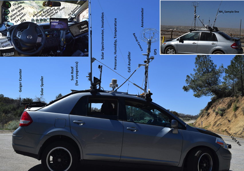
Figure 1. Photos of AMOG (AutoMObile trace Gas) Surveyor. Upper left inset shows cockpit.

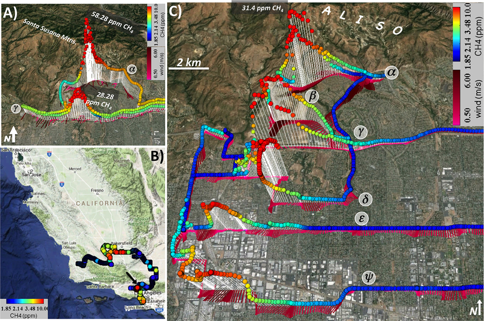
Figure 2. (A) Pre-survey methane (CH₄) concentrations and winds downwind of the Aliso Canyon leak, collected 05:06–05:39 PST, 13 November 2015. Peak plume transect concentrations labeled. (B) California map showing all collected data 13–14 November 2015. Black arrow shows Aliso Canyon location. (C) Methane, CH₄, and wind observations for the Aliso Canyon leak in the San Fernando Valley, CA, collected 10:40–15:10 PST, 13 November 2015. Note, CH₄ color bar is attenuated to capture spatial concentration structure near ambient. Data keys on panel.

Sample air is drawn down a ½″ Perfluoroalkoxy (PFA) Teflon sample line from 5 m above ground into a configurable range of gas analyzers by a high flow (30 ft³ min⁻¹) vacuum pump (Edwards, GVSP30). The sample line connects to several instruments including a Fast-flow, enhanced performance Greenhouse Gas Analyzer (FGGA), which uses Integrated Cavity Off Axis Spectrometer-Cavity Ring Down Spectrometer (ICOAS-CRDS) and measures CO₂, CH₄, and water vapor (H₂O) at up to 10 Hz (Model 911-0010, Los Gatos Research, Inc.).

A sonic anemometer (VMT700, Vaisala) mounted 1.4-m above the roof measures two-dimensional winds. Recent science AMOG Surveyor system improvements beyond Leifer et al. (2014) include a fast thermocouple (50416-T, Cooper-Atkins) and a high accuracy (0.2 hPa) pressure sensor (61320V RM Young Co.). Thermocouples (Type T) are digitized at ±0.03°C (CB-7018, Measurement Computing, MA), which also digitizes the solar insolation sensor at 16 bit and 1 Hz (CB-7017, Measurement Computing). Position information is critical to accurate real winds and is provided at 10 Hz by redundant (two) Global Navigation Satellite Systems (19X HVS, Garmin) that use the GLONASS, GPS, Galileo, and QZSS satellites for improved performance.

The use of real-time traffic and familiarity with the study area aids navigation, while real-time wind visualization can be used to ensure driving on upwind side of streets and highways. The impact of dense urban structures on winds can be reduced by filtering for specific open areas such as parking lots, fields, etc. in post-processing. Additionally, intersections with idling cars create local, near-surface exhaust clouds. This was addressed by timing approaches to intersections to allow idling cars and their emission clouds to flush downwind, and by collecting air samples at slow driving speed from 5-m height. Although, nocturnal data collection avoids many urban challenges (Leifer et al., 2013), the nocturnal urban atmosphere typically features low wind speeds and a very shallow PBL, making modeling highly challenging (Finn et al., 2008). An additional urban challenge arises from dense multi-story structures, where the road grid channels surface winds. However, once a plume diffuses above the structures it can drift freely but will re-enter the road grid through downward diffusion.

In situ surveys included the collection of vertical profile data to identify the PBL by leveraging nearby topography. Specifically, AMOG Surveyor drove into the nearby San Gabriel Mountains, ~10–20 km to the east. Profile surveys used small, sparsely trafficked roads. Still, there was some traffic, which was addressed by AMOG Surveyor pulling alongside the road for 1–2 min when catching up to a slower vehicle.

Plume Inversion and Uncertainty

There are two approaches to assess emissions, either by an assimilation inversion model based on a range of stationary station measurements (Jeong et al., 2012, 2013), or a direct assessment approach (White et al., 1976; Karion et al., 2013; Peischl et al., 2015). Direct assessment has advantages over inversion approaches. Specifically, direct approaches allow explicit evaluation of uncertainty with no need for an a-priori emission spatial distribution, nor for the ability to model accurately atmospheric transport. The latter two aspects challenge assimilation approaches, particularly for areas of complex topography, regions with poorly characterized (or unknown) sources. Furthermore, challenges arise where temporal variability in winds and emissions require data to be collected sufficiently rapidly with adequate data density to address fine-scale structure.

Total emissions (E) were estimated by two different direct approaches, a Gaussian plume inversion (E_Gauss) and a well-mixed PBL integration (E_Mixed).

Plume inversion was performed on purely east west transects (no north-south jogs). Inspection of the “clean” transects (γ and ε), i.e., transects that were purely east west without north-south jogs (dictated by road accessibility) used the curvefit tool in MatLab (Mathworks, MA) to fit dual Gaussian functions (Figure 2C) to the anomaly concentration (C′) for each transect. C′ was calculated from the average of the lowest values to the west of the plume (east of the plume, CH₄ concentrations were influenced by urban sources).

The Gaussian functions were used to segregate data between the different plumes and were not used in the Gaussian plume model. The dual plume character was consistent with observations at the most northerly roads that concentrations peaked in front of two canyons to the south of the source (Figure 2). This spatial structure was apparent in all transects. A sharp, narrow plume was fit to transect ε, which was assessed as having a local (non-Aliso) source, and was segregated out of C′ as used in the model.

Transect wind speeds were acceleration-filtered (>1 m s⁻²) and then rolling-median time-filtered (10-s time window). Finally, the upper 10% of wind speeds were used to estimate the wind speed based on the wind probability distribution for each transect. This accounts for the weaker winds reflecting the influence of buildings, trees, etc., and was validated during a vertical profile inter-comparison between AMOG Surveyor and an airplane data set collected in the Sierra Nevada Mountains. This approach also accounts for extending wind speeds from 3 to 10 m above ground heights (Leifer, unpublished data).

The Gaussian plume model is based on Hanna et al. (1982) and error minimized between the modeled and measured C′, for the along-wind, transverse, and vertical dimensions, x, y, z, respectively, to estimate E and is:

where h is plume origin height, u is wind speed, and σ_y and σ_z are given by:

from Hanna et al. (1982) for Briggs Turbulence and stability class three, and k is an added factor between zero and one that accounts for constraint of the plume's lateral dispersion due to topography after Bierly and Hewson (1962). Stability class three is unstable with strong solar insolation and moderate to strong winds. The emission height (h) was set at 150 m to address the plume's initial buoyant rise and injection at altitude. However, the flux is very weakly sensitive to h at the distances of the plume transects. Although, the source location was known, the origin for the Gaussian plume at downwind distance (D) was allowed to vary because the canyons have a “channelizing” effect on the plume, preventing lateral dispersion (Angell et al., 1972; Lamb et al., 1978). This is equivalent to a “virtual origin” for the plume close to the canyon mouth (where it exits onto the alluvial tilted plain of the north San Fernando Valley). The wind speed was ~4 m s for sunny conditions, thus, the inversion calculation used stability class three (Hanna et al., 1982). Table 1 provides Gaussian model parameters.

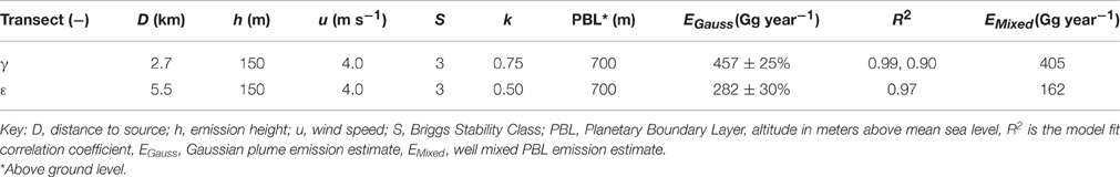
Table 1. Best scenario estimated flux and parameters.

The value of E for plume first was calculated by averaging E_Gauss for both transects with E_Mixed for transect ε and was 365 Gg CH₄ year⁻¹. However, a best estimate for E was calculated using a scenario approach (Shakhova et al., 2014), which also was used to derive the uncertainty (Supplementary Section Scenario Uncertainty Analysis). The scenario approach is a simplified Monte Carlo where the probability distribution function that normally would be sampled for the Monte Carlo simulations is assumed uniform, but quantized. For each scenario, low, observed, and high wind speeds of 3, 4, and 5 m s⁻¹, respectively, were chosen for the plume inversion, and represent the envelope of observations. This uncertainty scenario is based on the reality that wind speeds only are known (measured) at one point and time and not along the entire path of travel, over which they certainly vary; albeit, within limits. The scenarios also considered that the “source” distance is uncertain, as it is a “virtual distance,” due to the effect of topographic control on reducing the lateral turbulence (factor k). D was set at low, high, and best values of ±18.5% (±1 km at transect ε) for each of the two transects based on estimated reasonable limits for the location. For each of the nine scenarios run for each plume on each transect, the inversion algorithm (as above) minimized the error to derive the values for k and E_Gauss.

MODIS Aerosol Optical Depth

Satellite AOD from the Terra and Aqua MODIS satellites was downloaded and gridded from the satellite granule pixel locations to a uniform latitude-longitude coordinate system using the MatLab (v2015b, Mathworks, MA) sparse interpolation routine, (scattered interpolant) with the “natural” setting. This interpolation routine addresses the retrieval sparseness or non-uniformity of the AOD data, while also ensuring the interpolation goes through each data point. Data were sparse for a number of reasons, include clouds, quality flags, and no retrieval. Only data of the highest quality flag were used with successful retrieval density varying across the scene.

Weather Regional Forecast Model

To interpret the spatial distributions of AOD enhancements, the Weather Regional Forecast (WRF) model, version 3.6.1, was run in a series of four nested domains ranging from 36-km over Western US down to 1.3-km resolution, providing wind fields and PBL thicknesses over a domain covering the South Coast Air Basin that includes Aliso Canyon. The WRF model was run with time averaging adapted for atmospheric trace gas transport (Skamarock et al., 2008; Nehrkorn et al., 2010; Jeong et al., 2013) over California. Here, we employed boundary and initial conditions from the North American Regional Reanalysis (NARR) dataset (Mesinger et al., 2006). We parameterized WRF to use 50 vertical levels, applied the MYNN2 boundary layer physics (Nakanishi and Niino, 2006) and unified NOAH model for land surface properties (Chen and Dudhia, 2001). This minimizes errors in boundary layer meteorology. We computed each day of simulation in a separate 30-h run with an initial 6-h spin-up.

Results

Pre-survey Observations

Prior to the main survey, a pre-survey (Figure 2A) was performed at ~05:00 LT (Local Time) when traffic on Los Angeles highways is light. For example, heavy traffic prevents surveys on US-101 (both directions) after ~06:00 LT. The pre-survey was conducted to understand area survey constraints from traffic and terrain for predicted winds, which already exhibited Santa Ana wind strengths (u = 5 to >10 m s⁻¹) at altitudes above 400 m.

Pre-survey CH₄ concentrations to 58 part per million (ppm) were observed at 05:17 LT downwind of the principal canyons that guide plumes in the near field (transect α in Figure 2A). An extended weaker plume (CH₄ > 6 ppm) was observed to the east of the main plume, representative of nocturnal transport down a different canyon. At this hour (stably stratified, nocturnal wind patterns), strong Santa Ana winds were observed primarily in front of canyon outflows and showed significant spatial heterogeneity. Despite strong winds (to 9.7 m s⁻¹) and a source distance of several kilometers, these values were significantly higher than almost all surface observations obtained in tens of thousands of AMOG Surveyor data across Southern California.

Main Survey

Mobile surface survey data of the Aliso CH₄ plume were collected mid-morning, 13 November 2015 to characterize the plume's downwind evolution (Figure 2C). By mid-morning, online weather information (http://www.weatherunderground.com) indicated that the nocturnal weather patterns had shifted to daytime conditions. The survey repeatedly transected the plume at multiple downwind distances from the source (y) from 2 to 9 km (Figure 3).

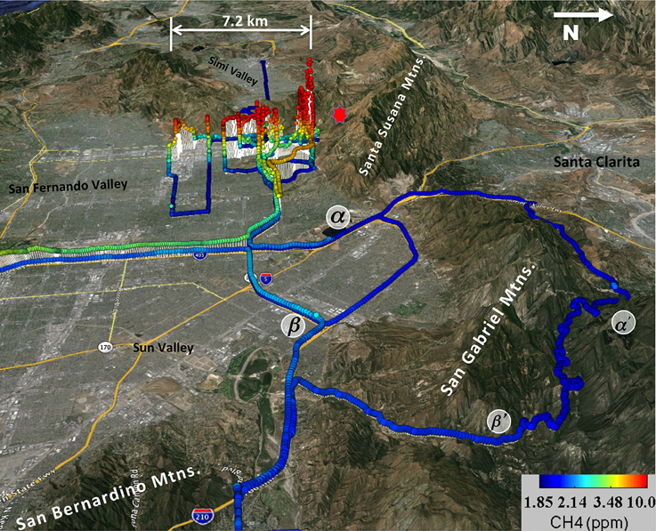
Figure 3. Methane (CH₄) data collected in the San Fernando Valley and up into the San Gabriel Mountains to collect atmospheric vertical profile information. Red star shows leak location. Data key, vertical profile locations (α–α′ is ascent profile, β′–β is descent profile), and size scale on figure.

Atmospheric Profile Characterization

Aside from collecting downwind data for the Aliso Canyon leak, three vertical profiles were collected into the San Bernardino Mountains (Figure 3) to elevations of 830 m and 1.4 km above mean sea level (AMSL, all altitudes are AMSL). Two profiles were conducted before the survey, and one afterwards while transiting to near the Edwards Air Force Base in the Mojave Desert. The profiles (Figure 4) showed air in the lower Los Angeles Basin had enhanced CH₄ and CO₂, largely constrained to a layer extending to ~570 m, although it is important to note the influence of winds down the I-5 Pass (α–α′). However, the temperature profiles both showed that AMOG Surveyor entered distinct upper level air at about 700 m, where the relative humidity also showed a minimum. Also, there was a slight (~50 ppb) enhanced CH₄ in a thin layer at this altitude, which also was the top of an inversion layer, observed on the descending transect. Note, the more enhanced CO₂ anomalies from 400 to 450 m altitude are influenced by traffic on the I-5; however, the small road driven up into the San Bernardino Mountains had almost no traffic.

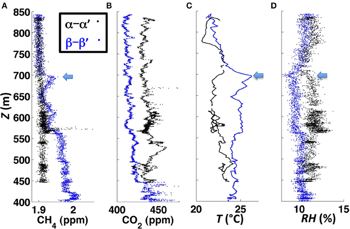
Figure 4. AMOG altitude (z) profile data into the San Bernardino Mountains for (A) methane (CH₄), (B) carbon dioxide (CO₂), (C) temperature (T), and (D) relative humidity (RH). Blue arrows highlight features showing top of the planetary boundary layer. Vertical profiles (α–α′ is ascent profile, β′–β is descent profile) are labeled as identified on Figure 3. Data key on (A).

Vertical profiles were collected in the San Bernardino Mountains before and after the main survey and showed a stable PBL (690–720 m), which grew only a few dozen meters over several hours (Figures 3, 4). Although, the PBL was identified below the leak altitude, Santa Ana winds follow topography (Hughes and Hall, 2010), driving the plume downslope, while also minimizing the potential for significant buoyant rise.

Plume Inversion

Plume inversion (Hanna et al., 1982) based on error minimization was conducted on the two downwind “clean” transects (γ, ε)—east-west that were along a straight pathway—in some cases, available roads prevented straight transects. The inversion used a model that incorporated topographic control on plume dispersion due to being in a canyon (Drivas and Shair, 1974; Lamb et al., 1978). These transects were well described by a dual Gaussian function (Table 1, Figure 5). The dual plume character was consistent with observations at the most northerly roads that concentrations peaked in front of two canyons to the south of the source (Figure 2), a spatial plume structure that was apparent in all transects.

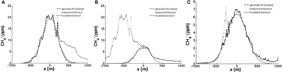
Figure 5. (A) Methane (CH₄) anomaly concentration (CH^′₄) profiles, with respect to transverse distance (x) Gaussian functional fit to data, and Gaussian plume model fit for (A) transect γ for main plume, and (B) transect γ fit for secondary plume, and (C) fit for the plume on transect ε. Data key on figure.

The closer transect (γ) had good agreement between E_Mixed and E_Gauss, within the uncertainty of E_Gauss, where E_Gauss is the Gaussian plume inversion and E_Mixed assumes a well-mixed PBL. E_Mixed used the observed 700 m PBL (Figure 3) and assumed constant winds with altitude. Observed wind profiles for Santa Ana winds show fairly uniform distribution with height on the downslope flow portions of the plume, although Santa Ana winds weaken dramatically once out onto the plains, where the wind profile becomes significantly non-uniform (Hughes and Hall, 2010). This likely explains the worse agreement between E_Mixed and E_Gauss.

Additional issues arise from the lateral wind profile. Within and near the canyon, including the Porter Ranch community, winds and CH₄ exhibit similar large-scale spatial structure under strong topographic influence; as evidenced by “k” being much less than one (k = 1 implies a non-topographically constrained plume). However, for the more distant transect, the plume sprawls over areas with distinct wind regimes. Plume inversion confirmed the extreme strength of the Aliso Canyon leak emissions (Table 1).

MODIS Aerosol Optical Depth

For this analysis, MODIS, Terra and Aqua, satellite data were used for 13 November 2015 for Southern California, although a longer time set of these data were obtained and reviewed. The specific aerosol product used was the Level 2, “Image Optical Depth Land and Ocean,” product (MOD04_3K), for the MODIS data collection 6 and were downloaded from NASA LAADS (Level 1 and Atmosphere Archive and Distribution System). Specifically, MODIS 250-m reflectance and the 3 km AOD for 0.55 nm products (Levy et al., 2010) as well as the cloud mask and aerosol type were downloaded and then post-processed in MatLab (Mathworks, MA). Maps of AOD were visualized with a linear color scale to emphasize variations for low columns, and any quality-flagged pixels were set transparent. Maps of AOD then were brought into Google Earth to overlay with in situ data.

The AOD map (Figure 6) shows notable enhancements in the Los Angeles Basin and San Fernando Valley with low AOD for mountainous regions to the north and northwest of Los Angeles. A map with the AOD contrast enhanced shows spatial structural details that highlight the presence of enhanced AOD in the coastal mountain passes (red arrows, Figure 7). Note these mountain passes are not transportation routes. The fine structure in the AOD map suggests that transport veers sharply to the east offshore, based on an east-west spatial structure (below green arrows, Figure 7). Figure 7 has high contrast enhancement to illustrate AOD spatial structure in the mountain passes and over the ocean.

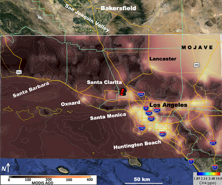
Figure 6. Aerosol Optical Depth (AOD) from MODIS for 2055 UTM, 13 November 2015, for southern California. Also shown is the Aliso Canyon plume methane (CH₄). Data keys on figure.

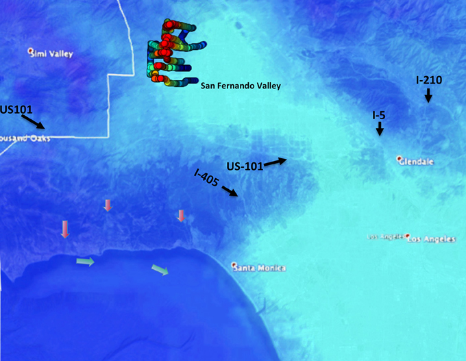
Figure 7. Contrast enhanced to show overall MODIS Aerosol Optical Depth (AOD) structure for 13 November 2015 for northwest Los Angeles and the San Fernando Valley. AOD contrast highly saturated to bring out spatial structure in passes and over oceans. Pale green arrows lie immediately north of the offshore AOD structure, which exhibits an east-west orientation and is shown to illustrate airflows. Major traffic arteries through mountain passes are labeled with relevant highway and black arrows. Red arrows shows three different plume outflows, the easternmost corresponding to downwind of the Aliso Canyon leak plume. Methane (CH₄) data shown for spatial reference. See Figure 3 for CH₄ data and CH₄ data key. See Figure 6 for AOD data with AOD data key.

Modeled Winds and Plume Transport

Observed plume trajectory overlapped well with MODIS AOD (Figure 6), which clearly showed enhanced AOD in passes from the San Fernando Valley to the Pacific Ocean. The contours of AOD (Figure 6) strongly suggest canyon outflow to the Pacific Ocean and offshore, followed by easterly onshore transport across the Santa Monica Bay and toward coastal Los Angeles communities. The possibility that the offshore spatial structure related to transport was investigated further through WRF numerical simulations (Figure 8), which showed that southward winds through the passes (continuing in the same direction as observations) veered to the east over the Pacific Ocean. Specifically, WRF simulations captured the shift from offshore Santa Ana winds to prevailing westerly winds. Additionally, WRF showed that this wind pattern persisted into later in the day (14 November 2015, 0100 UTM) allowing time to transport Aliso Canyon leak CH₄ back onshore.

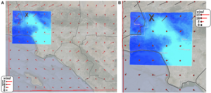
Figure 8. Weather Regional Forecast (WRF) modeled surface (100 m AGL) winds, for 13 November 2015, 2100 UTM. (A) Large area view showing winds for much of the Los Angeles Basin. Also shown is the Aerosol Optical Depth (AOD) map from Figure 7 for reference only. (B) Zoomed in study area.

Discussion

Improving Transport Understanding

Events such as the Aliso Canyon leak are tracer experiments such as once were common with SF₆ (Lamb et al., 1978). Today, new in situ sensors and remote sensing technology can leverage such events to understand better atmospheric transport. In the case of the Aliso Canyon leak, the release occurred in the complex wind flow patterns of a megacity sprawling over terrain with notable topographic relief.

Plume dilution was slow for Santa Ana wind conditions (Figure 2C), which are frequent in Los Angeles during the fall and winter seasons (Abatzoglou et al., 2013). Specifically, C_CH4 (y ~ 2 km) decreased by just half at y ~ 10 km. The explanation partly lies in the constraining impact of canyon walls, which reduces significantly the lateral diffusion rate (k < 1) by topographic forcing (Angell et al., 1972; Lamb et al., 1978). In future chemical release accidents of a highly toxic gas, dilution with distance cannot be a priori assumed to lower risk rapidly, with even distant communities potentially remaining at risk.

The Aliso Canyon leak surface survey required many hours to characterize the local plume (to y ~ 10 km) and PBL. Airplane in situ is far faster (at least for a highly maneuverable airplane), characterizing plumes above the surface and even over the ocean, but invariably intersects the many controlled airspaces in a megacity like Los Angeles. Moreover, it is the surface concentration that has serious consequences for human health. Thus, surface data can add to airborne data at far lower logistical costs.

Satellite Observations

Ideally, remote sensing can help. The ideal response instrument would be a geostationary instrument with high spatial resolution and selectivity for the released gas, providing near real time observations of fate trajectory and emission strength. Geostationary instruments can dwell on an area, unlike low earth orbit satellites (Zhang and Kerle, 2008).

To characterize a strong CH₄ leak, such as from Aliso, a CH₄ mapping satellite with coverage and resolution comparable to the OCO2 satellite (Crisp et al., 2010), which observes only CO₂ (at 70-m resolution), is needed. Unfortunately, no CH₄ satellite instrument with kilometer or better resolution currently orbits, nor is one planned for near-future launch. Moreover, there currently is no such space-based instrument for any of the numerous toxins (e.g., benzene, toluene, etc.) that could be released. Airborne remote sensing has an important advantage in that it avoids entering toxic plumes where in situ measurements could pose unacceptable risks to responders.

Numerical models can aid response decisions and thereby help fill the lack of a satellite trace gas instrument for plume mapping. However, wind flow complexity related to topography provides major challenges to interpretation of both in situ data and numerical models. Thus, validation is critically important. Atmospheric aerosols, which are readily remote sensed from space, provide a good tracer to validate model predictions. Satellite trajectory tracing of aerosols (Engel-Cox et al., 2005) applies directly to refinery or other chemical plant fires where aerosol generation accompanies hazardous gas emissions (Khan and Abbasi, 1999). Nevertheless, because urban aerosols are common (Hayes et al., 2013), they provide a readily available air mass tracer even for incidents that do not include fire, and thus do not generate aerosols. Additional aerosol map cross-validation can be provided from the space-based lidar, CALIOP (Cloud-Aerosol Lidar with Orthogonal Polarization). The CALIOP sensor has been used to study volcanic plumes (Vernier et al., 2013). Additional validation can come from airborne in situ and remote sensing of aerosols.

The Santa Ana winds drive a southward airflow across and out of the San Fernando Valley through mountain passes, highlighted in the MODIS AOD (Figure 7). This validated the WRF simulations and illustrates how important topography is to atmospheric transport in the Los Angeles Basin (Drivas and Shair, 1974). Notably, strong AOD enhancements occurred in the main transport corridors that traverse passes within the Los Angeles Basin, such as US-101, l-I5, and I-215 (Figure 7). Given that normal rush hour traffic grinds to a standstill, the suitability of evacuation routes that use these passes, which also may conduct chemical plumes, merits consideration. Ancillary data, such as winds, are key, as elevated AOD does not mean transport. For example, traffic within the passes and in situ chemical production certainly produce local aerosols.

A southward offshore flow, which is typical for Santa Ana winds (Trasviña et al., 2003), was illustrated by the MODIS AOD. This flow then veered toward the prevailing eastwards wind direction ~10 km offshore. This drove the plume toward densely populated coastal communities near Los Angeles airport. If the disaster had been a refinery emission of highly toxic gas, validation of numerical model predictions would be key for responders assessing which communities needed the most immediate evacuation.

Incorporating satellite aerosol remote sensing data into disaster response plans and decision-making requires short latency and rapid revisit times: MODIS Level 1 data latency is 70 min, but Level 2 aerosol products have 1 day latency. Therefore, near real-time products need development. Geostationary aerosol products from GOES (Geostationary Operational Environmental Satellite; Weber et al., 2010) or the planned TEMPO (Tropospheric Emissions: Monitoring of Pollution) mission can provide half hour or hourly daylight data for North America, respectively (Zoogman et al., in press). The TEMPO mission also will provide other potentially contributory satellite data related to air quality trace gases, such as ozone. This study showed a need for improvements in urban real-time AOD retrieval algorithms, where AOD density (despite high quality flags) was non-ideal.

Conclusion

Characterization of the plume from Aliso Canyon was performed by surveys with the AutoMObile trace Gas (AMOG) Surveyor, which measured mobile surface in situ CH₄ and winds under Santa Ana conditions. Analysis yielded an estimated annualized emission rate of 365 ± 30% Gg CH₄ year⁻¹. Plume dispersion was constrained significantly by topography, reduced by up to a factor of two. Local topography was leveraged by AMOG Surveyor to provide vertical profiles that were used to identify the PBL at ~700 m. Observations showed the plume was transported toward passes in the coastal Santa Monica Mountains. To understand the far field fate, satellite AOD was mapped and suggested the plume flowed offshore before veering eastwards back toward shore. This interpretation was validated by comparison with a numerical model.

This study demonstrated and validated the novel application of satellite aerosol remote sensing for disaster response. Currently and for the near future, there is no satellite instrument that can map any of the numerous toxins (e.g., benzene, toluene, etc.) that a chemical release disaster can emit. Thus, satellite aerosol remote sensing can provide a readily available proxy tool to provide synoptic scale information on the fate of co-transported toxins from a release.

The use of a car-based survey platform was novel and has logistical advantages in terms of ease of mobilization. However, car systems are constrained to roads, unlike airplanes, which can easily fly vertical profiles. Ideally, combined surface and airborne data are collected to provide a complete characterization of the atmosphere from the surface where injury occurs to the top of the PBL. Given that airborne data were not collected in tandem with this AMOG Surveyor deployment, local topography was leveraged to provide vertical profiles.

Aerosol remote sensing is of high priority to climate, safety, health, and atmospheric corrections for satellite instruments. Thus, including a priori science requirements for disaster response science requirements into the design considerations for future aerosol remote sensing instruments and platforms (airborne and space-based) can improve understanding of urban atmospheric transport. Leveraging these remote sensing tools requires ensuring disaster response scientific requirements contribute to instrumentation and platform design in terms of sensitivity, resolution, and revisit times, (satellite and airborne). Equally important, aerosol products need incorporation into response planning. This would allow future instruments to contribute to mitigating the serious consequence of chemical release disasters.

Author Contributions

IL field collected data, analyzed the satellite data and wrote the manuscript. CM analyzed the in situ data and made figures. JF helped data collection. XC ran WRF. MF analyzed WRF winds and edited the manuscript and made figures. JM edited the manuscript, DG contributed to the manuscript organization and structure.

Conflict of Interest Statement

The authors declare that the research was conducted in the absence of any commercial or financial relationships that could be construed as a potential conflict of interest.

Acknowledgments

We thank the editorial suggestions of Robert Corell, Global Environment Technology Foundation, and Robert Leifer (Department of Energy, retired). We thank Seongeun Jeong for providing Weather Research Forecast model wind output. IL, CM, and JF were supported by the Research and Analysis Program of the NASA Earth Science Division, grants NNX13AM21G and NASA Applied Science Disasters Program, NNX16AI07G. MF, XC were supported by a grant from the California Energy Commission's Natural Gas Research Program to the Lawrence Berkeley National Laboratory under contract DE-AC02-36605CH11231. JM was supported by the NASA Applied Science Program, Disasters Area.

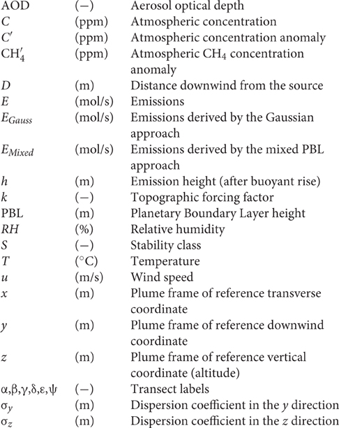
Nomenclature

Supplementary Material

The Supplementary Material for this article can be found online at: https://www.frontiersin.org/article/10.3389/fenvs.2016.00059

References

Abatzoglou, J. T., Barbero, R., and Nauslar, N. J. (2013). Diagnosing Santa Ana winds in Southern California with synoptic-scale analysis. Weather Forecast. 28, 704–710. doi: 10.1175/WAF-D-13-00002.1
Angell, J. K., Pack, D. H., Machta, L., Dickson, C. R., and Hoecker, W. H. (1972). Three-dimensional air trajectories determined from Tetroon flights in the planetary boundary layer of the Los Angeles Basin. J. Appl. Meteorol. 11, 451–471.
Angevine, W. M., Brioude, J., Mckeen, S., Holloway, J. S., Lerner, B. M., Goldstein, A. H., et al. (2013). Pollutant transport among California regions. J. Geophys. Res. 118, 6750–6763. doi: 10.1002/jgrd.50490
Benjamin, D. (2009). Best practices in chemical emergency response preparedness and incident management:: rendering comprehensive models through the utilization of streaming meteorological data, active sensor readings, complex terrain compensation, and GIS intelligence. J. Chem. Health Safety 16, 26–29. doi: 10.1016/j.jchas.2008.09.001
Bierly, E. W., and Hewson, E. W. (1962). Some restrictive meteorological conditions to be considered in the design of stacks. J. Appl. Meteorol. 1, 383–390.
Brandt, A. R., Heath, G. A., Kort, E. A., O'sullivan, F., Pétron, G., Jordaan, S. M., et al. (2014). Methane leaks from North American natural gas systems. Science 343, 733–735. doi: 10.1126/science.1247045
Cao, Y., and Fovell, R. G. (2016). Downslope windstorms of San Diego County. Part I: a case study. Month. Weather Rev. 144, 529–552. doi: 10.1175/MWR-D-15-0147.1
Chen, F., and Dudhia, J. (2001). Coupling an advanced land surface–Hydrology model with the Penn State–NCAR MM5 modeling system. Part II: Preliminary model validation. Month. Weather Rev. 129, 587–604. doi: 10.1175/1520-0493(2001)129<0587:CAALSH>2.0.CO;2
Conley, S., Franco, G., Faloona, I., Blake, D. R., Peischl, J., and Ryerson, T. B. (2016). Methane emissions from the 2015 Aliso Canyon blowout in Los Angeles, CA. Science 351, 1317–1320. doi: 10.1126/science.aaf2348
Crisp, D., Boesch, H., Brown, L., Castano, R., Christi, M., Connor, B., et al. (2010). OCO (Orbital Carbon Observatory) - 2: Level 2 Full Physics Retrieval Algorithm Theoretical Basis. Pasadena, CA: Jet Propulsion Laboratory.
Dobashi, R. (2014). Fire and explosion disasters occurred due to the Great East Japan Earthquake (March 11, 2011). J. Loss Prev. Process Ind. 31, 121–126. doi: 10.1016/j.jlp.2014.03.001
Drivas, P. J., and Shair, F. H. (1974). A tracer study of pollutant transport and dispersion in the Los Angeles area. Atmos. Environ. 8, 1155–1163. doi: 10.1016/0004-6981(74)90049-3
Edinger, J. G. (1959). Changes in the depth of the marine layer over the Los Angeles Basin. J. Meteorol. 16, 219–226.
EIA (2014). Natural Gas Annual Respondent Querry System, Field Level Storage Data (Annual). Washington, DC: U.S. Energy Information Administration.
Engel-Cox, J. A., Hoff, R. M., and Haymet, A. D. J. (2004). Recommendations on the use of satellite remote-sensing data for urban air quality. J. Air Waste Manag. Assoc. 54, 1360–1371. doi: 10.1080/10473289.2004.10471005
Engel-Cox, J. A., Young, G. S., and Hoff, R. M. (2005). Application of satellite remote-sensing data for source analysis of fine particulate matter transport events. J. Air Waste Manage. Assoc. 55, 1389–1397. doi: 10.1080/10473289.2005.10464725
Farrell, P., Leifer, I., and Culling, D. (2013). Transcontinental methane measurements: Part 1. A mobile surface platform for source investigations. Atmos. Environ. 74, 422–431. doi: 10.1016/j.atmosenv.2013.02.014
Finn, D., Clawson, K. L., Carter, R. G., Rich, J. D., and Allwine, K. J. (2008). Plume dispersion anomalies in a nocturnal urban boundary layer in complex terrain. J. Appl. Meteorol. Climatol. 47, 2857–2878. doi: 10.1175/2008JAMC1864.1
Gurjar, B. R., Butler, T. M., Lawrence, M. G., and Lelieveld, J. (2008). Evaluation of emissions and air quality in megacities. Atmos. Environ. 42, 1593–1606. doi: 10.1016/j.atmosenv.2007.10.048
Hanna, S. R., Briggs, G. A., and Hosker, R. P. Jr. (1982). Handbook on Atmospheric Diffusion. Springfield, VA: Technical Information Center, U.S. Department of Energy.
Hayes, P., Ortega, A., Cubison, M., Froyd, K., Zhao, Y., Cliff, S., et al. (2013). Organic aerosol composition and sources in Pasadena, California, during the 2010 CalNex campaign. J. Geophys. Res. 118, 9233–9257. doi: 10.1002/jgrd.50530
Heintzenberg, J. (1989). Fine particles in the global troposphere A review. Tellus 41B, 149–160. doi: 10.1111/j.1600-0889.1989.tb00132.x
Hong, S.-Y., Noh, Y., and Dudhia, J. (2006). A new vertical diffusion package with an explicit treatment of entrainment processes. Month. Weather Rev. 134, 2318–2341. doi: 10.1175/MWR3199.1
Howarth, R. W., Santoro, R., and Ingraffea, A. (2011). Methane and the greenhouse-gas footprint of natural gas from shale formations. Clim. Change 106, 679–690. doi: 10.1007/s10584-011-0061-5
Hughes, M., and Hall, A. (2010). Local and synoptic mechanisms causing Southern California's Santa Ana winds. Clim. Dyn. 34, 847–857. doi: 10.1007/s00382-009-0650-4
IPCC (2007). “Climate change 2007: synthesis report,” in Contribution of Working Groups I, II, and III to the Fourth Assessment Report of the Intergovernmental Panel on Climate Change,” eds R. K. P. Core Writing Team and A. Reisinger (Geneva: IPCC).
IPCC (2014). “Working Group 1 Contribution to the IPCC Fifth Assessment Report Climate Change 2013,” in The Physical Science Basis, eds T. Stocker, Q. Dahe, and G.-K. Plattner (Geneva: International Panel on Climate Change).
Jeong, S., Hsu, Y.-K., Andrews, A. E., Bianco, L., Vaca, P., Wilczak, J. M., et al. (2013). A multi-tower measurement network estimate of California's methane emissions. J. Geophys. Res. 118, 11339–11351. doi: 10.1002/jgrd.50854
Jeong, S., Zhao, C., Andrews, A. E., Bianco, L., Wilczak, J. M., and Fischer, M. L. (2012). Seasonal variation of CH4 emissions from central California. J. Geophys. Res. 117, D11306. doi: 10.1029/2011JD016896
Jones, C., Fujioka, F., and Carvalho, L. M. V. (2010). Forecast skill of synoptic conditions associated with Santa Ana Winds in Southern California. Month. Weather Rev. 138, 4528–4541. doi: 10.1175/2010MWR3406.1
Karion, A., Sweeney, C., Pétron, G., Frost, G., Michael Hardesty, R., Kofler, J., et al. (2013). Methane emissions estimate from airborne measurements over a western United States natural gas field. Geophys. Res. Lett. 40, 4393–4397. doi: 10.1002/grl.50811
Khan, F. I., and Abbasi, S. A. (1999). Major accidents in process industries and an analysis of causes and consequences. J. Loss Prev. Process Ind. 12, 361–378. doi: 10.1016/S0950-4230(98)00062-X
Krstic, N., and Henderson, S. B. (2015). Use of MODIS data to assess atmospheric aerosol before, during, and after community evacuations related to wildfire smoke. Remote Sens. Environ. 166, 1–7. doi: 10.1016/j.rse.2015.05.017
Lamb, B. K., Lorenzen, A., and Shair, F. H. (1978). Atmospheric dispersion and transport within coastal regions—Part I. Tracer study of power plant emissions from the Oxnard Plain. Atmos. Environ. 12, 2089–2100. doi: 10.1016/0004-6981(78)90164-6
Lamb, B. K., Mcmanus, J., Shorter, J., Kolb, C., Mosher, B., Harriss, R., et al. (1995). Development of atmospheric tracer methods to measure methane emissions from natural gas facilities and urban areas. Environ. Sci. Technol. 29, 1468–1479. doi: 10.1021/es00006a007
Langford, A. O., Senff, C. J., Alvarez, R. J., Banta, R. M., and Hardesty, R. M. (2010). Long-range transport of ozone from the Los Angeles Basin: a case study. Geophys. Res. Lett. 37, L06807. doi: 10.1029/2010GL042507
Leen, J. B., Yu, X. Y., Gupta, M., Baer, D. S., Hubbe, J. M., Kluzek, C. D., et al. (2013). Fast in situ airborne measurement of ammonia using a mid-infrared off-axis ICOS spectrometer. Environ. Sci. Technol. 47, 10446–10453. doi: 10.1021/es401134u
Leifer, I., Culling, D., Schneising, O., Farrell, P., Buchwitz, M., and Burrows, J. (2013). Transcontinental methane measurements: Part 2. Mobile surface investigation of fossil fuel industrial fugitive emissions. Atmos. Environ. 74, 432–441. doi: 10.1016/j.atmosenv.2013.03.018
Leifer, I., Lehr, W. J., Simecek-Beatty, D., Bradley, E., Clark, R., Dennison, P., et al. (2012). State of the art satellite and airborne marine oil spill remote sensing: application to the BP Deepwater Horizon oil spill. Remote Sens. Environ. 124, 185–209. doi: 10.1016/j.rse.2012.03.024
Leifer, I., Melton, C., Manish, G., and Leen, B. (2014). Mobile monitoring of methane leakage. Gases Instrum. 2014, 20–24.
Levy, R. C., Remer, L. A., Kleidman, R. G., Mattoo, S., Ichoku, C., Kahn, R., et al. (2010). Global evaluation of the Collection 5 MODIS dark-target aerosol products over land. Atmos. Chem. Phys. 10, 10399–10420. doi: 10.5194/acp-10-10399-2010
Lindell, M. K., and Perry, R. W. (1997). Hazardous materials releases in the Northridge Earthquake: implications for seismic risk assessment. Risk Anal. 17, 147–156. doi: 10.1111/j.1539-6924.1997.tb00854.x
Lu, R., and Turco, R. P. (1995). Air pollutant transport in a coastal environment—II. Three-dimensional simulations over Los Angeles basin. Atmos. Environ. 29, 1499–1518. doi: 10.1016/1352-2310(95)00015-Q
Lu, R., Turco, R. P., and Jacobson, M. Z. (1997). An integrated air pollution modeling system for urban and regional scales: 1. Structure and performance. J. Geophys. Res. 102, 6063–6079.
Mckain, K., Down, A., Raciti, S. M., Budney, J., Hutyra, L. R., Floerchinger, C., et al. (2015). Methane emissions from natural gas infrastructure and use in the urban region of Boston, Massachusetts. Proc. Natl. Acad. Sci. U.S.A. 112, 1941–1946. doi: 10.1073/pnas.1416261112
Mesinger, F., Dimego, G., Kalnay, E., Mitchell, K., Shafran, P. C., Ebisuzaki, W., et al. (2006). North American Regional Reanalysis. Bull. Am. Meteorol. Soc. 87, 343–360. doi: 10.1175/BAMS-87-3-343
Meyers, M. P., and Steenburgh, W. J. (2013). “Mountain weather prediction: phenomenological challenges and forecast methodology,” in Mountain Weather Research and Forecasting: Recent Progress and Current Challenges, eds K. F. Chow, F. J. S. De Wekker, and J. B. Snyder (Dordrecht: Springer), 1–34.
Nakanishi, M., and Niino, H. (2006). An improved Mellor Yamada level-3 model: its numerical stability and application to a regional prediction of advection fog. Boundary Layer Meteorol. 119, 397–407. doi: 10.1007/s10546-005-9030-8
Nehrkorn, T., Eluszkiewicz, J., Wofsy, S., Lin, J., Gerbig, C., Longo, M., et al. (2010). Coupled weather research and forecasting–stochastic time-inverted lagrangian transport (WRF–STILT) model. Meteorol. Atmos. Phys. 107, 51–64. doi: 10.1007/s00703-010-0068-x
Peischl, J., Ryerson, T. B., Aikin, K. C., De Gouw, J. A., Gilman, J. B., Holloway, J. S., et al. (2015). Quantifying atmospheric methane emissions from the Haynesville, Fayetteville, and northeastern Marcellus shale gas production regions. J. Geophys. Res. 120, 2119–2139. doi: 10.1002/2014jd022697
Piccot, S. D., Beck, L., Srinivasan, S., and Kersteter, S. L. (1996). Global methane emissions from minor anthropogenic sources and biofuel combustion in residential stoves. J. Geophys. Res. 101, 22757–22766. doi: 10.1029/95JD01920
Schmidt, A., Leadbetter, S., Theys, N., Carboni, E., Witham, C. S., Stevenson, J. A., et al. (2015). Satellite detection, long-range transport, and air quality impacts of volcanic sulfur dioxide from the 2014–2015 flood lava eruption at Bárdarbunga (Iceland). J. Geophys. Res. 120, 9739–9757. doi: 10.1002/2015jd023638
Shakhova, N., Semiletov Igor, P., Leifer, I., Sergienko, V., Salyuk, A., Kosmach, D., et al. (2014). Ebullition and storm-induced methane release from the East Siberian Arctic Shelf. Nat. Geosci. 7, 64–70. doi: 10.1038/ngeo2007
Shen, S. S., and Lewis, P. E. (2011). “Deepwater Horizon oil spill monitoring using airborne multispectral infrared imagery,” in SPIE (Orlando, FL), 80480H-80481-80480H-80416.
Shie, R.-H., and Chan, C.-C. (2013). Tracking hazardous air pollutants from a refinery fire by applying on-line and off-line air monitoring and back trajectory modeling. J. Hazard. Mater. 261, 72–82. doi: 10.1016/j.jhazmat.2013.07.017
Sigurdsson, H., Devine, J. D., Tchua, F. M., Presser, F. M., Pringle, M. K. W., and Evans, W. C. (1987). Origin of the lethal gas burst from Lake Monoun, Cameroun. J. Volcanol. Geotherm. Res. 31, 1–16. doi: 10.1016/0377-0273(87)90002-3
Skamarock, W. C., Klemp, J. B., Dudhia, J., Gill, D. O., Barker, D. M., Huang, X. Z., et al. (2008). A Description of the Advanced Research WRF Version 3. Boulder, CO: National Center for Atmospheric Research, Mesocale and Microscale Meteorology Division.
Thompson, D., Leifer, I., Bovensman, H., Eastwood, M., Fladeland, M., Frankenberg, C., et al. (2015). Real-time remote detection and measurement for airborne imaging spectroscopy: a case study with methane. Atmos. Meas. Tech. 8, 1–46. doi: 10.5194/amt-8-4383-2015
Trasviña, A., Ortiz-Figueroa, M., Herrera, H., Cosıo, M. A., and González, E. (2003). ‘Santa Ana’ winds and upwelling filaments off Northern Baja California. Dyn. Atmos. Oceans 37, 113–129. doi: 10.1016/S0377-0265(03)00018-6
Tratt, D. M., Buckland, K. N., Hall, J. L., Johnson, P. D., Keim, E. R., Leifer, I., et al. (2014). Airborne visualization and quantification of discrete methane sources in the environment. Remote Sens. Environ. 154, 74–88. doi: 10.1016/j.rse.2014.08.011
Vernier, J. P., Fairlie, T. D., Murray, J. J., Tupper, A., Trepte, C., Winker, D., et al. (2013). An advanced system to monitor the 3D structure of diffuse volcanic ash clouds. J. Appl. Meteorol. Climatol. 52, 2125–2138. doi: 10.1175/JAMC-D-12-0279.1
Weber, S. A., Engel-Cox, J. A., Hoff, R. M., Prados, A. I., and Zhang, H. (2010). An improved method for estimating surface fine particle concentrations using seasonally adjusted satellite aerosol optical depth. J. Air Waste Manage. Assoc. 60, 574–585. doi: 10.3155/1047-3289.60.5.574
Wecht, K. J., Jacob, D. J., Sulprizio, M. P., Santoni, G. W., Wofsy, S. C., Parker, R., et al. (2014). Spatially resolving methane emissions in California: constraints from the CalNex aircraft campaign and from present (GOSAT, TES) and future (TROPOMI, geostationary) satellite observations. Atmos. Chem. Phys. 14, 8173–8184. doi: 10.5194/acp-14-8173-2014
White, W. H., Anderson, J. A., Blumenthal, D. L., Husar, R. B., Gillani, N. V., Husar, J. D., et al. (1976). Formation and transport of secondary air pollutants: Ozone and aerosols in the St. Louis urban plume. Science 194, 187–189.
Yacovitch, T. I., Herndon, S. C., Pétron, G., Kofler, J., Lyon, D., Zahniser, M. S., et al. (2015). Mobile laboratory observations of methane emissions in the Barnett Shale Region. Environ. Sci. Technol. 49, 7889–7895. doi: 10.1021/es506352j
Young, S., Balluz, L., and Malilay, J. (2004). Natural and technologic hazardous material releases during and after natural disasters: a review. Sci. Total Environ. 322, 3–20. doi: 10.1016/S0048-9697(03)00446-7
Zhang, Y., and Kerle, N. (2008). “Satellite remote sensing for near-real time data collection,” in Geospatial Information Technology for Emergency Response, Vol. 6, eds S. Zlatanova and J. Li (London: Taylor & Francis Group), 75–102.
Keywords: methane, disaster response, remote sensing, aerosol, plume, atmospheric transport, megacity
Citation: Leifer I, Melton C, Frash J, Fischer ML, Cui X, Murray JJ and Green DS (2016) Fusion of Mobile In situ and Satellite Remote Sensing Observations of Chemical Release Emissions to Improve Disaster Response. Front. Environ. Sci. 4:59. doi: 10.3389/fenvs.2016.00059
Received: 26 March 2016; Accepted: 22 August 2016;
Published: 22 September 2016.
Edited by:
William Albert Lahoz, Norwegian Institute for Air Research, NorwayReviewed by:
Bijoy Vengasseril Thampi, Science Systems and Applications, Inc, USARobert David Bornstein, San Jose State University, USA
Copyright © 2016 Leifer, Melton, Frash, Fischer, Cui, Murray and Green. This is an open-access article distributed under the terms of the Creative Commons Attribution License (CC BY). The use, distribution or reproduction in other forums is permitted, provided the original author(s) or licensor are credited and that the original publication in this journal is cited, in accordance with accepted academic practice. No use, distribution or reproduction is permitted which does not comply with these terms.
*Correspondence: Ira Leifer, Ira.Leifer@bubbleology.com