Primary frequency response from hydrogen-based bidirectional vector coupling storage: modelling and demonstration using power-hardware-in-the-loop simulation

Highlights

• A detailed model of vector coupling storage incorporating the pertinent factors associated with its activities is devised.

• Implementation of vector coupling storage for frequency response service is demonstrated using Power-Hardware-In-the-Loop simulation and Digital Twin technique.

• Performance of vector coupling storage in the integrated energy system, for frequency response application, is evaluated.

1 Introduction

The rationale for integrating networks across energy vectors has strengthened in recent years due to benefits including enhanced flexibility and security of energy supply (Clegg and Mancarella, 2015), reduced carbon emission, optimised efficiency, and reduced operational cost (Abeysekera et al., 2016). Several coupling components, such as utility-scale electrolysis and fuel cell stacks, can facilitate this integration. The government of the United Kingdom has allocated carbon budgets to reach net-zero emissions by 2050 (HM Government, 2023). Achieving this goal will require high penetrations of renewable energy sources in the energy system, which will reduce the inertia of the electrical network. This will make the system more vulnerable to more frequent and severe frequency events, resulting in load shedding (Aupetit and Pokluda, 2018), secondary photovoltaic tripping (Australian Energy Market Operator, 2016), generation shedding (Banks et al., 2017), and interconnector tripping (Australian Energy Market Operator, 2019). These problems can be addressed using appropriately designed control measures to manage the system frequency. The energy required for frequency response services could be delivered via renewable energy sources (Yan et al., 2015) and large-scale energy storage (Greenwood et al., 2017; Ghazavi Dozein and Mancarella, 2019). However, in future smart low-carbon integrated energy systems (IESs), hydrogen is expected to become a major player in the energy storage market and could participate in frequency regulating services (Alexander and Spliethoff, 2018).

Existing energy system integration studies focus on the techno-economic-environmental impact of energy network integration without considering the impact—positive or negative—on system frequency (Troncoso and Newborough, 2011; Ursúa et al., 2013; Reza Hosseini et al., 2018; Reza Hosseini et al., 2020; Saedi et al., 2020; Reza Hosseini et al., 2021). For example, the authors in (Troncoso and Newborough, 2011; Ursúa et al., 2013) discussed the co-deployment of small-scale polymer electrolyte membrane (PEM) hydrogen electrolysers with wind or solar generators to reduce the curtailment of renewable energy. In (Alshehri et al., 2019), a dynamic model of a plant composed of fuel cells and electrolysers is employed to evaluate the contribution of this plant to frequency response. However, this paper did not use a dynamic electrolyser model, focusing instead on fuel cells alone. In addition, the power converter needed to couple the electrolyser with the grid was not considered, so the interaction between the electrolyser and power system dynamics cannot be captured. It has been demonstrated in (Tuinema et al., 2020) how converter constraints may negatively affect the ability of electrolysers to deliver primary frequency response (PFR). A simplified dynamic model of an electrolyser, in which the converter is assumed to be ideal and uncontrolled, is presented in (Tuinema et al., 2020). Because of this assumption, the dynamic behaviour required to deliver frequency response cannot be appropriately represented.

A dynamic model of a grid-scale, PEM-type hydrogen electrolyser is presented in (Ghazavi Dozein et al., 2021). This electrolyser can be used for short-term frequency response in large-scale power systems; the impact of providing this service on the converter control loop is explicitly considered, as are the design of the load-frequency controller and the size and location of the electrolyser. The benefits of the response provided by the electrolyser (from a system perspective) are quantified. However, the energy flow is unidirectional, with the electrolyser acting only as a flexible load to contribute to frequency regulation.

1.1 Research gaps and contributions

This paper suggests a novel bidirectional Hydrogen based vector coupling storage (VCS) to provide primary frequency response in IES. The structure of the VCS is shown in Figure 1. This structure includes a grid-scale electrolyser, grid-scale fuel cells, and Hydrogen storage. In this structure, the energy flow is bidirectional. The grid-scale electrolyser is interfaced with the electrical network through a power converter. This electrolyser converts electrical energy to hydrogen, which is stored in a storage. The storage capacity limit is managed by injecting hydrogen into the gas network. If the storage capacity is reached and the electrolyser is required to operate, the valve connecting the Hydrogen storage to the gas network will open and the excess Hydrogen will be injected into the gas network. The fuel cells, which can convert hydrogen stored in the storage to electricity, are also interfaced with the electrical network through a power converter. This VCS system will contribute to frequency regulation by absorbing and injecting power into the electricity system. The Hydrogen level in the buffer will be controlled and kept within a specified range to meet the requirement of any frequency incident.

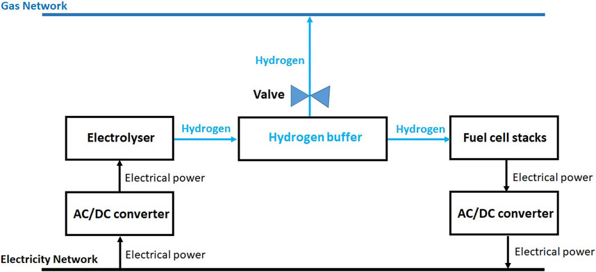
FIGURE 1. The structure of the bidirectional hydrogen-based VCS to provide PFR service.

The VCS can deliver PFR in a short duration, however, this period depends on the component involved in correcting the frequency deviation. The active power step response of the electrolyser and fuel cells are in the order of 1–2 s (Nikiforow et al., 2018; Alshehri et al., 2019; Tuinema et al., 2020), but the response of the VCS system was unknown and this was, therefore, important to assess. To represent the power converter accurately, this paper used a physical converter via power hardware in the loop (PHIL); this allowed accurate measurement of the power converter’s effect on the frequency response controller. PHIL is a technique for developing and assessing intricate, embedded systems in real-time, permitting real-power hardware to interface with computer models (Guillaud et al., 2015; Sayfutdinov et al., 2016). For example, PHIL simulation was used in (Sayfutdinov et al., 2016) to evaluate the developed voltage regulation algorithm.

Digital Twin (DT) techniques (Werner et al., 2018; Nguyen et al., 2022) can be employed to address VCS integration challenges by enabling prototype validation and integration testing. The DT is defined as a digital model with a two-way automated data flow from the physical object to the digital model (Werner et al., 2018; Borth et al., 2019; Nguyen et al., 2022). The authors in (Werner et al., 2018) provided a categorical classification of different types of digital twins. The work in (Nguyen et al., 2022) demonstrated the use of DT and PHIL to assess the impact of renewable energy resources on the electrical distribution network. (Nguyen et al., 2022) also discussed the challenges facing the DT and explored strategies and architectures that tackle these challenges. The authors exemplified this viewpoint of DT in relation to cyber-physical systems and the Internet of Things, using instances from the domains of smart grid and smart buildings. In this paper, we propose a state-of-the-art pre-integration assessment method, combining the DT and PHIL techniques, to examine how VCS integration affects IES. The PHIL will represent the power grid and the power converters interfacing the VCS. The DT represents the VCS. This method enables the development of a realistic deployment environment for evaluating the VCS’s efficiency, time response, and VCS’s impact on the stability of the electricity network. In fact, there has been extensive work conducted in the research community on real-time simulation and PHIL testing environments. However, the DT has unique features for linking data between the physical system and the virtual model, and the performance can be significantly affected by the data transmitting rate and the computational capacity of the platform hosting the DT. In other words, the computational capacity must be sufficient to execute the DT within each specified time step. These unique features present special needs for the testing environment and the existing testing setup has not been designed for, and thus not adequate to suit the purpose.”

The main contributions of this paper are:

•Contribution 1: The bidirectional hydrogen-based VCS design and dynamic model as a Digital TwinThis paper presents a novel, flexible VCS system which can be used to provide bi-directional frequency control to an electricity transmission network. A digital twin (DT) for this VCS system is developed. This DT considers all the key parameters affecting the behaviours of the main components of VCS such as the pressure and temperature.

•Contribution 2: Integration of the Digital Twin of the VCS with the power system using PHILIn this paper, we propose a novel method for evaluating VCS by combining DT and PHIL in a state-of-the-art virtual-physical environment. With this method, not only can the effects of VCSs be assessed, but the entire deployment environment can be taken into account, where realistic or even extreme cases can be simulated. The assessment method consists of three major steps:

1. In its desired deployment condition, the VCS impact on the electrical grid is examined via the DT of VCS.

2. The desired deployment environment (i.e., the Great Britain power system) is then created and configured through the PHIL technique.

3. The global impact of the newly added VCS is then investigated as it propagates through the DT in real time to the PHIL setup.The designed testing environment considered the challenges of harmonising the DT execution speed and the rates of data exchanges between the DT and the deployment environment. Section 3 outlines the overall structure of the configuration that integrates PHIL and DT principles to establish a virtual-physical environment for comprehensive VCS evaluation. According to the authors’ knowledge, no previous work has combined the DT and PHIL techniques to assess the integration of VCS into the IES.

•Contribution 3: VCS Speed of responseIn the context of primary frequency control, response time is a crucial factor. In this work, we evaluate that speed by developing a dynamic, DT prototype of the VCS and connecting it to a real DC/AC power converter via PHIL. Previous work has considered the speed of response of individual components or a subset of components which would be part of a more holistic vector coupling storage system (Nikiforow et al., 2018; Alshehri et al., 2019; Tuinema et al., 2020). In addition, the power converter, which needed to couple the electrolyser with the grid, was not considered. Converter constraints may negatively affect the ability of the electrolyser to deliver primary frequency response (Tuinema et al., 2020), and therefore the accurate dynamic behaviour of the converters must be considered in the evaluation of the speed of response of VCS.

1.2 Research questions

Using DT and PHIL simulation, the following research questions will be investigated in this paper:

• How quickly can a VCS respond to a frequency incident by delivering power?

• How can the hydrogen buffer be controlled to guarantee that there is enough energy available to meet the PFR service obligations?

• Can the VCS mitigate severe frequency events?

• Is droop control used to control battery energy storage systems delivering PFR service still appropriate to control a bidirectional hydrogen-based VCS?

2 Dynamic modelling of the bidirectional hydrogen-based vector coupling storage as a DT

Figure 2 depicts the VCS model, which includes models of the PEM electrolyser, fuel cells, and hydrogen storage. These models are presented in Section 2.1– respectively.

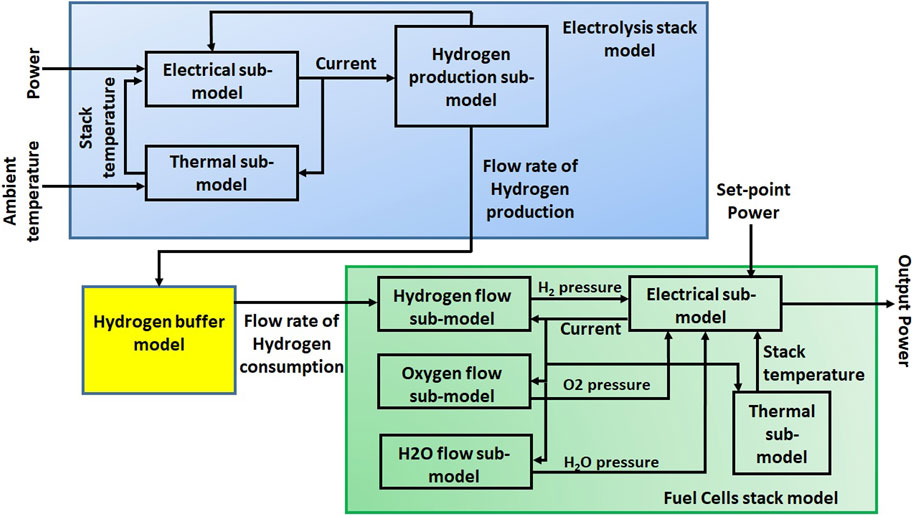
FIGURE 2. Diagram of the VCS model.

2.1 Electrolysis stack model

The fast dynamics of the electrolysis process are the PEM electrolysers’ most attractive capacity, making them particularly well-suited for applications involving frequency response. The adjustment of electricity consumption levels through ramping up and down can be accomplished within a relatively brief span of time (in the order of seconds). Moreover, partial loading levels below the rated capacity can be sustained for long duration without adversely affecting the system’s performance. Hence, this technical capability must be reflected in the electrolyser model.

In fact, the PEM electrolysis stack model comprises three interconnected sub-models: electrical, thermal, and Hydrogen production. The most relevant interactions between these sub-models for frequency response application must be considered. It can be seen in Figure 2 that there is no feedback from the hydrogen production sub-model and the electrical sub-model. This means that the hydrogen production process does not affect the electrical dynamics (Ghazavi Dozein et al., 2021).

2.1.1 Electrolyser’s electrical sub-model

The electrolysis stack’s electrical sub-model can be simplified as an equivalent circuit, which comprises a voltage source (representing the reverse voltage of the electrolysis stack, V_rev), an internal resistance (R_i) that accounts for various internal electrical losses, and a parallel combination of the mass transport resistance (R_m) and the over-potential capacitor (C_op) (Sarrias-Mena et al., 2015; Ghazavi Dozein et al., 2021), all connected in series. When a sudden change in the stack current i(t) occurs, the parallel component in the circuit represents the EDL phenomenon that obstructs the flow of electrons at the interface between the electrode and electrolyte. This obstruction delays the response of the electrolyser to the change in current (Ghazavi Dozein et al., 2021). All three components are dependent on the stack temperature (T) and pressure (p), as indicated in Eqs 1–3. The electrolysis pressure must be kept close to the desired level for safety reasons and to guarantee stable hydrogen production. Hence, Eqs 1–3 can assume that the stack pressure remains constant.

the equations presented here describe various parameters related to the VCS system. The stack voltage at a given time is denoted by U_t(t), while e_rev0 represents the reference value for reverse voltage, and R_io is the internal resistance at standard temperature T₀ and pressure p₀. The voltage drop across the parallel combination of R_m and C_op is denoted by V_Cop. The temperature coefficient of resistance is represented by dR_t, while k and F denote the fitting curve parameter and Faraday constant, respectively (Sarrias-Mena et al., 2015).

2.1.2 Thermal sub-model of the electrolyser

Eq. 4 (Sarrias-Mena et al., 2015) presents the thermal energy balance in the electrolysis stack, which forms the basis of the thermal sub-model.

in Eq. 4, the left-side term represents the thermal energy storage in the stack where C_stack is the heat capacity of the electrolyser stack (J/K), $\dot{Q_{\mathit{loss}}}$ represents the heat lost to the surroundings, and $\dot{Q_{\mathit{cool}}}$ is the heat loss to the cooling peripheral. $\dot{Q_{\mathit{gen}}}$ is found using Equation 5 (Miland, 2005),

where n_c is the number of cells in electrolysis stack; U_m is the thermal neutral cell voltage [V]; and η_e is the electrolyser electricity efficiency. In this equation, the P_EZ = U_t·i(t) represents the power supplied to the electrolyser from the electrical network.

The linearized heat losses $(\dot{Q_{\mathit{loss}}})$ around the ambient temperature T₀ can be expressed as (Miland, 2005; Ghazavi Dozein et al., 2021).

where R_stack is the thermal resistance of the electrolyser stack (K/W); $\dot{m_{DI}}$ and C_w represent, respectively, the mass flow water in the cooling system (Kg/s) and specific heat capacity of water (kJ/Kg·K). Substituting Eqs 5–7 into Eq. 4 and then applying Laplace transformation yields the transfer function of the thermal sub-model:

The transfer function given in Eq. 8 is a first-order function with time constant ${\tau }_{th}=\frac{C_{\mathit{stack}}}{\dot{m_{DI}}·C_w+\frac{1}{R_{\mathit{stack}}}}$ (s).

2.1.3 Hydrogen production sub-model

The active power input to the electrolyser P_EZ = U_t·i(t) is used in the electrolysis stack to produce hydrogen. The dynamic behaviour of the stack current affects the amount of hydrogen produced by the electrolysis stack instantaneously, as shown in Eq. 9, (Alexander and Spliethoff, 2018; Ghazavi Dozein et al., 2021):

where $m_{H_2}$ is the hydrogen production rate $\left(\frac{N{m}^3}{s}\right)$, η_F is Faraday efficiency (C/kmol), N is the number of electrolysis cells electrically connected in series and operated at a current i(t). The coefficient k_c = 4,841.4 converts mole/s to Nm³/s (Alexander and Spliethoff, 2018; Ghazavi Dozein et al., 2021).

2.1.4 Validating the dynamic model of PEM electrolyser using real-world data

In this paper, we have validated the dynamic response of the electrolyser model by comparing it to field measurements obtained from a 1 MW pilot electrolyser located in the northern Netherlands (Tuinema et al., 2020). The experiments investigated the ramp-up and down capabilities of the electrolyser and its ability to maintain partial loading. The simulation results of our electrolyser model are presented in Figure 3 alongside the experimental results from (Tuinema et al., 2020). The parameters of the electrolysis cell model are: e_rev0 = 1.476 [V], R_io = 0.326 [Ω], R_m = 1 [Ω], C_op = 1 [nF], p₀ = 1 [atm], T₀ = 20°C, k = 0.0395, dR_t = −3.812e-3, and F = 96,487. The electrolyser stack consists of an array of electrolysis cells. In this array, the number of series and parallel cells are respectively 275 and 3,700. Figures 3A, B show that the pilot electrolyser took less than 2 s to adjust the amount of electricity used by ramping hydrogen production up or down (Tuinema et al., 2020), and shutting down entirely only takes a few seconds. Additionally, significant periods of time can be spent maintaining partial loading levels in relation to the rated capacity (Tuinema et al., 2020). Figures 3C, D demonstrate that the model of the electrolyser can realistically reproduce the response produced by the actual electrolyser.

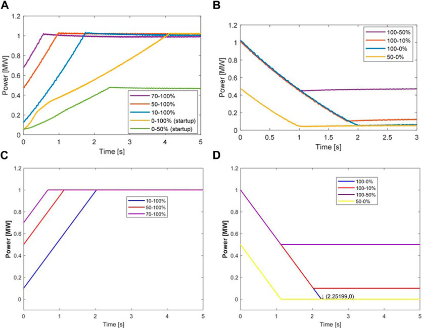
FIGURE 3. Validation of the dynamic model of PEM electrolyser: Pilot electrolyser response to variations in operation set point (Tuinema et al., 2020) (A) ramp up, and (B) ramp down; Response to variations in operation set point obtained from the model presented in this paper, (C) ramp up, and (D) ramp down.

2.2 Fuel cells model

Various models have been proposed in the literature to describe the steady-state and dynamic characteristics of fuel cells. Complex models based on electro-chemical equations (Amphlett et al., 1996; Wang et al., 2005; Andújar et al., 2008; San Martín et al., 2014) show how the reactions in the stack occur. Simpler models use mathematical approximations, while others use semi-empirical or empirical data and model fitting, as discussed in (Kong et al., 2005; Hou et al., 2010; Restrepo et al., 2014). For this paper, the PEM fuel cell model focuses on the dynamics of the stack and considers the parameters affecting these dynamics. The model that describes the dynamic behaviour of the PEM fuel cell stack is composed of three interconnected sub-models: electrical, thermal, and hydrogen consumption. These are presented in Section 2.2.1–2.2.4.

The following assumptions have been made to enable tractable modelling of the PEM fuel cell.

• The fuel cell receives the hydrogen and air as gases, which are uniformly distributed and behave ideally. They are supplied at a constant pressure.

• To model the thermodynamic characteristics of the stack, an ambient temperature of 25°C and a constant specific heat capacity for the stack are assumed, along with the average temperature of the stack.

• Individual fuel cell characteristics can be combined to constitute a fuel cell stack, and numerous stacks can be combined to represent a utility-scale fuel cell system.

2.2.1 Electrical sub-model of the fuel cells

The model relies on Nernst’s equation and Ohm’s law to calculate the voltage across the anode and cathode in the fuel cell stack, as expressed in the following equation:

where N_FC is the number of cells per stack, E₀ is the no-load voltage of a cell estimated in [V], R is the universal gas constant [J/lmol/K], F is Faraday’s constant [C/kmol], T is the stack temperature in [K], and r_int is the internal resistance [Ω]. The term r_int·I_FC in Eq. 10 represents the electrical losses produced in the internal resistance of the stack and B. ln (C·I_FC) represents the electrochemical activation losses due to the Tafel slope. Both losses are dependent on the temperature of the stack, which will is described in section 2.2.3. The current produced by the fuel cells stack will be determined from the input power set-point and the voltage of the fuel cells stack: I_FC = P_{FC−setpoint}/U_FC. In Eq. 10, $p_{H_2}$, $p_{O_2}$, and $p_{H_{2}O}$ are the partial pressures of the hydrogen, Oxygen, and water estimated in [atm], respectively.

The internal resistance of the fuel cell stack in Eq. 10 is dependant on the stack temperature (T) as shown in Eq. 11,

where r₀ is the pre-exponential factor [Ω], and E_a,R is the activation energy [J/mol]. In addition, the tafel slope (B) in Eq. 10 is a function of stack temperature, as shown in Eq. 12,

where B₀ is the pre-exponential factor [V], and E_a,A is the activation energy [J/mol].

2.2.2 Sub-models of gas pressures in the fuel cell stack

Both hydrogen and oxygen flow through the fuel cell electrodes at given partial pressures. These gases are assumed ideal, so their partial pressures can be quantified using the ideal gas equation. Applying this law to the hydrogen yields Eq. 13:

where V_an and $m_{H_2}$ represent the volume of the anode channel and the moles of the hydrogen in this channel, respectively. Eq. 13 can be applied for all the gases. Assuming the pressure drop across the electrode channels is negligible, this will give the relationship between the hydrogen flow from the buffer and the partial pressure of the hydrogen, which can be expressed as:

where $q_{H_2}$ and $k_{H_2}$ are the molar flow of hydrogen estimated in [kmol/s] and hydrogen tank molar constant [kmol/atm/s].Eq. 14 can be used to find the derivative of its partial pressure:

where $q_{H_2}$, and $q_{H_2}^r$ are, respectively, the hydrogen input flow, and the hydrogen reaction flow rate estimated in [kmol/s]. This hydrogen flow is also related to stack current:

where I_FC is the stack current [A] and K_t is the modelling constant [kmol/s/A]. Substituting Eq. 15 in Eq. 16, the derivative of partial pressure can be written in the s-domain as follows:

in the same way, the derivative of the partial pressure of the Oxygen and water can be written in the s-domain as follows:

where $q_{O_2}$, $k_{O_2}$, and ${\tau }_{O_2}$ represent, respectively, the molar flow of Oxygen [kmol/s], the Oxygen valve molar constant [kmol/atm/s], and Oxygen time constant [s].

where $q_{\left.H_2\right)}$, $k_{H_{2}O}$, and ${\tau }_{H_{2}O}$ represent, respectively, the molar flow of water [kmol/s], the water valve molar constant [kmol/atm/s], and water time constant [s].

2.2.3 Thermal sub-model of the fuel cells

In (Alshehri et al., 2019), the fuel cell stack’s thermal sub-model is described, which relates the stack’s temperature to its initial and steady-state temperature values when the current is modified during a given time step.

where T₁ and T₂ are the initial and final allowed temperatures of the fuel cell stack. H_t and mc_p represent the heat transfer coefficient [W/C°] and heat capacitance coefficient of the stack [J/C°]. The values of the parameters in Eq. 20 are given in (Alshehri et al., 2019) and estimated using empirical data fitting presented in (Soltani and Taghi Bathaee, 2010).

2.2.4 Hydrogen consumption sub-model

The fuel cell stack uses hydrogen as a feedstock and the dynamic of the stack current is affected by the amount of hydrogen consumed by the electrolysis stack instantaneously, as shown by Eq. 16.

2.2.5 Validating the dynamic model of PEM fuel cell

The presented model has been validated using experimental data from a Nexa PEM fuel cell with a capacity of 1.2 kW and current range of 46 A and a voltage range of 26 V, as well as empirical data (Soltani and Taghi Bathaee, 2010). Step loads were applied to the model as shown in Figure 4A, to quantify its dynamic characteristics. The results are shown alongside experimental curves in Figure 4B. The model response shown in Figure 4C, is in good match with the experimental data. Increases in the load current reduce the output voltage due to voltage losses within the internal resistance. Simulations have shown that the fuel cell’s output voltage responds almost instantly to changes in load, but with an overshoot or undershoot that decreases exponentially over time. Therefore, the output power also changes rapidly in response to load variations.

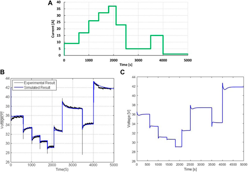
FIGURE 4. Validation of the PEM fuel cell stack dynamic model: (A) simulated current profile, (B) experimental voltage response (Soltani and Taghi Bathaee, 2010), (C) voltage response obtained from the model presented in this paper.

2.3 Model of hydrogen storage

Hydrogen storage is a tank which stores hydrogen produced by the electrolysis stack and is used to supply the fuel cell stack. As shown in Figure 1, the valve can affect the level of hydrogen in the tank. Hydrogen from the storage can be injected into the gas network if the tank was already full. Hence, the level of hydrogen (LoH) in the storage can be expressed as follows:

in Eq. 21, S_v and S are integer variables to express the operational status of the valve, and the combination of the electrolyser and the fuel cells stacks: S_v = 1 when the valve is open, otherwise S_v = 0; S = 1 when the electrolyser is operating and the fuel cell stack is not, and S = 0 when the fuel cell stack is operating and the electrolyser is not. q_H is the hydrogen flow input to the fuel cells stack given in Eq. 16. $m_{H_2}$ is the Hydrogen production rate of the electrolyser, given by Eq. 9. K₁ and K₂ are the conversion coefficients from Nm³/s and kmol/s to MW, respectively. TC stands for the nominal hydrogen tank capacity estimated in MWh and ΔT_s is the time step estimated in (s).

2.4 Control law of the VCS

This paper also proposes to adopt the droop control scheme suggested by National Grid in the UK for controlling battery energy storage systems delivering PFR service for use with VCS. Figure 5 shows the droop control used to control the VCS. This figure shows that the VCS can contribute to the regulation of both over- and under-frequency events. The electrolyser provides over-frequency droop control, its power input increasing by ΔP_EZ to $P_{max}^{EZ}$ if the frequency (f) is larger than (f₁). The fuel cells provide the under-frequency response and their power input increases by ΔP_FC to $P_{max}^{FC}$ if the frequency (f) is less than (f₂). The electrolyser was operated to adjust the level of Hydrogen (LoH) in the buffer when the frequency is within the range [f₁,f₂].

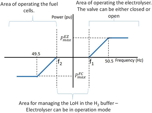
FIGURE 5. The response curve of the VCS for the PFR response.

3 Experimental investigation using PHIL

This section outlines the methodology for two experiments designed to guide the development of PFR service for VCS systems and address the research questions introduced in the previous section. The first experiment involves using high-resolution frequency data from the Great Britain (GB) network to evaluate the performance of a VCS system in response to real-world dynamic frequency data. In the second experiment, a simplified model of the GB power system was used in real-time to interact with the laboratory network and the DT of the VCS via a power converter. The second experiment investigates the effects of the VSC system’s response to frequency events resulting from a mismatch between supply and demand.

3.1 Laboratory setup and the implemented control system

Newcastle University established a Smart Grid Laboratory with an aim to merge the comprehensive scope of simulation and the detailed specificity of experimentation. This goal was achieved through the utilization of a flexible power conversion system (FPCS) and a real-time simulator for performing PHIL studies, along with a programmable DC source for simulating the VCS structure depicted in Figure 1. The VCS behaviour, regulated by the models described in Section 2, was replicated by this DC source. This meant that the emulator followed the ramp rates defined by the mathematical models of the electrolyser and the fuel cell. The VCS emulator was interfaced to the laboratory network’s 415 V busbar through a DC/AC power converter, which was controlled by a real-time target computer. This target computer also runs and hosts the DT of the VCS, which must be able to process the frequency measurement and generate the power set-point, within the defined time step. In this work, the model representing the VCS, given in Section 2, has been constructed in Simulink, which is then used to generate executable code. This code is then combined with the control system of the DC/AC power converter. The executable code of the DT calculates the set point of the VCS and sends it to the controller of the power converter. This last one controls the power injection/absorption from/to the bidirectional programmable DC source. The controller of the power converter is also built in Simulink, and this controller is then used to generate the executable code of the controller. The codes of the DT and the controller of the power converter are synchronised, and run at fixed time steps (50 μs).

To supply variable voltages and frequencies in real-time, a flexible 30 kVA AC/AC power converter energized the laboratory network. Variable frequencies were generated using both historical data and a simplified frequency response model for Great Britain’s power system, as described in the following paragraph. Figure 6 illustrates the setup of the laboratory for these experiments. The VCS controller with PFR algorithm was implemented as a Matlab script in the Simulink (TM) model that carried out the low-level control for the DC/AC converter. Additionally, a feedback loop was integrated into the overall controller to manage the LoH. A voltage waveform measured at the coupling point between the AC/DC converter and the laboratory network was subjected to a phase lock loop (PLL). This allowed the frequency to be measured. The DT data resolution is determined by the inherent measurement rate from the PLL. It is important to highlight that the controller of the AC/AC power converter runs at fixed time steps (50 μs). Ensuring the real-time characteristics of the DT is achieved through maintaining a consistent operation time-step and sampling frequency.

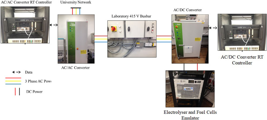
FIGURE 6. An illustration of the equipment interaction used in the laboratory setting for the research reported in this paper.

The controller of the VCS took a reading of both the frequency and the LoH at each time step. The controller would issue a new set point to correct the LoH by running the electrolyser if necessary in the case that the frequency was found to be within the regulatory limitations. The PFR droop curve in Figure 5 was used to calculate the power set-point if the frequency exceeded the limitations. This control algorithm is illustrated in Figure 7.

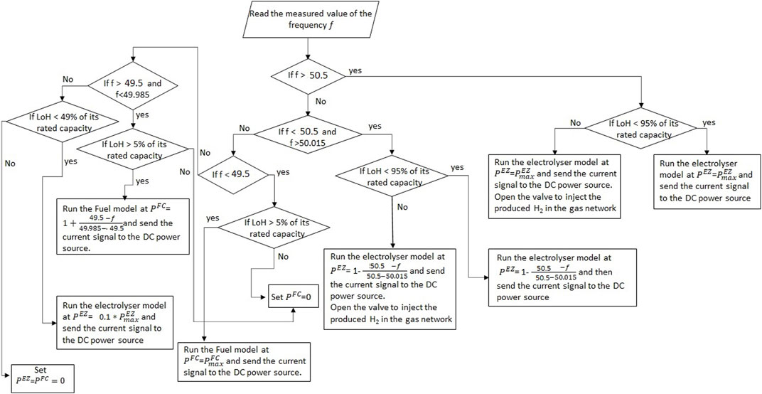
FIGURE 7. The control algorithm used to deliver the PFR and maintain the LoH greater than 49% of its hydrogen buffer capacity when the frequency within the dead band shown in Figure 5 where f₁ = 50.015 Hz and f₂ = 49.985 Hz.

3.2 Experimental design

This paper offers a valuable contribution to the field by integrating the DT of the VCS system with the power system using PHIL to demonstrate the capability of VCS system to respond to transient frequency changes with real power output—both historical and recorded in GB transmission network and generated by a power system model.

The simplified frequency response model of the GB power system, as shown in Figure 8 (Grigsby, 2007; Hassan, 2014), can be used to describe the dynamic relationship between generation and demand. This relationship can be quantified by the imbalance between generation and demand (ΔP_dev) or the frequency deviation (Δf). The equation for ΔP_dev, as defined by Eq. 22, yields a positive value when the demand is greater than the generation.

where H and D are the system inertia and damping constants, respectively. To model the current generation mix, H, is adjusted to 7.0 s (National Grid and ESO, 2019). Damped load has an effect on the system, as indicated by the damping constant, D. In the simulation, it is set to 1.0 p.u., which corresponds to a percentage change in demand for a 1% shift in frequency (Grigsby, 2007).

Within the GB system, frequency response providers are represented by two aggregated generators. The first generator, Gen₁, is a set of generators that provide primary frequency response, whereas the second generator, Gen₂, provides both primary and secondary frequency responses. Each generator connected at the transmission level and providing frequency response was required by the grid code to have a 3–5 percent governor droop (National Grid ESO, 2023). The factors G₁ and G₂ define each generator’s contribution to providing the frequency response. The generators’ dynamics are represented by three transfer functions illustrated in Figure 8. To improve the frequency control performance, a transient droop compensator, outlined in (Samarakoon et al., 2011), is employed. The governor and turbine are modeled using their time constants T_G and T_T, respectively, and Gen₂ has an extra controller to facilitate a secondary response. All the relevant simulation parameters are listed in Table 1 (Cheng et al., 2015; Bian et al., 2017).

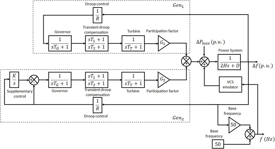
FIGURE 8. Simplified model of GB power system.

TABLE 1. Parameters of the simplified model of GB power system.

3.3 Experiment I—Response to historical frequency data

The setup used in the experiment is presented in Figure 9. The AC/AC converter received historical system frequency as input and reproduced this on the laboratory network. The VCS emulator (Regatron emulator) then responded to this frequency according to the frequency control depicted in Figure 7 and to its dynamic model given in Section 2. To obtain measurements, transducers were positioned at the AC/AC and AC/DC power converter’s grid interface. The objective of the experiment was to quantify the response time of the VCS system experimentally.

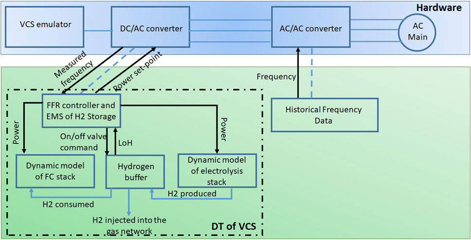
FIGURE 9. Laboratory setup and software used for Experiment I.

The historical system frequency data used in this experiment are for the transmission network in the GB and cover the period from April 2021 to May 2022 with a 1-s resolution. National Grid ESO has made these data accessible to the public in order for potential PFR suppliers to evaluate the viability of their systems. These data were analysed in order to determine the most likely operating regime of a VCS system that is responsible for providing PFR services before the results of this experiment were presented.

The system frequency is predominantly within the range of 49.8–50.2 Hz, as illustrated in Figure 10; the frequency was less than 49.8 Hz and just above 50.2 Hz, respectively, 0.0484% and 0.0448% of the time. 52.74% of the time, the frequency was within 0.05 Hz of the nominal value; however, only 13% of the time was it within 0.015 Hz. In this paper, the dead band shown in Figure 5 is ±0.015 Hz around the nominal frequency. This range was chosen as more interventions are required from the VCS to respond to the frequency deviation. This will allow for assessing the dynamic response of the VCS.

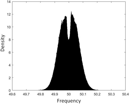
FIGURE 10. A histogram of the GB frequency transmission network during the period from April 2021 to May 2022.

3.4 Experiment II—Responding to frequency events

The setup of this experiment is illustrated in Figure 11. In this figure, the grid emulator is the simplified model of the GB power system shown in Figure 8. This model is developed in Simulink (TM) and used to generate executable code. The code is then combined with the controller of the AC/AC power converter to energise the laboratory network with the frequency profile generated by the GB power system model. The controller of the AC/AC power converter includes PI controllers to ensure zero-steady state error (i.e., ensuring high accuracy), and improve settling time. The executable codes of the model of the GB power system and the power converter’s controller are hosted by a real-time target computer. This target computer runs the executable codes at fixed steps (50 µs). As shown in Figure 11, these two executable codes exchange the values of the frequency and the power injected/absorbed by the VCS. The information exchange is also illustrated in Figure 8.

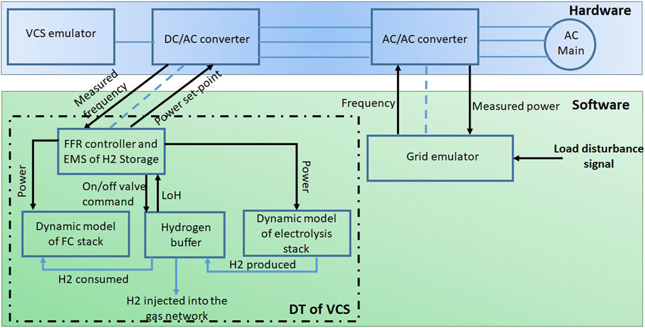
FIGURE 11. Experiment II—Real-time response to simulated frequency events—Setup of the laboratory and software.

Step changes in demand were used to generate transient frequency events. These events were designed in such a way that the resulting frequency deviation would exceed the limits at which a response is required (±0.015 Hz). The impact of the frequency event was emulated by the GB power system model, with the resulting frequency signal being sent to the AC/AC converter and reproduced on the lab network.

The frequency response curve was used to determine how the laboratory VCS system would respond to the frequency deviation. The VCS response was measured and sent to the grid emulator as shown in Figure 8, helping to correct the power system frequency. The power response from the VCS was scaled up before being sent into the grid emulator, making the VCS system in the laboratory behave as a huge VCS system or a collection of many small VCS systems. To figure out how well different penetrations of VSC would fix frequency deviations, a set of scaling factors was used. Regarding the scaling process of the VCS, the model of the VCS is first updated to correspond to the new size of the VCS (the number of cells/stacks and their interconnection). After calculating the power set point by the VCS model, this value will be sent to the controller of the DC/AC power converter which interfaces the VCS emulator with the laboratory network. The controller measures the network voltage, calculates the current value, and then scaled this value to be within the operational range of the VCS emulator [−20A, +20 A]. The controller of the DC/AC power converter also includes PI controllers to ensure the stability and accuracy of the power exchange between the VCS emulator and the laboratory network. The DT of the VCS and the controller of the DC/AC power converter are hosted by a real-time target computer. This target computer also runs the executable codes at fixed steps (50 µs). To close the loop, the input signal in the GB power system model, which corresponds to the measured value of the VCS power, is scaled up to match the value calculated by the DT. These experiments were conducted with the primary objective of experimentally evaluating the effectiveness of various levels of PFR response in mitigating severe frequency events.

4 Experimental results and discussion

In this section, the results of conducted experiments utilising the methodology mentioned in Section 3, the historical frequency data, and the frequency control system depicted in Figure 7 are presented.

4.1 Open loop response to historical frequency data

Based on the experiment description given in section 3.3, samples from the historical system frequency data for the transmission network in the GB, covering the period from April 2021 to May 2022, have been used in this experiment. Each sample is composed of 800 frequency values, and consequently, the sample size corresponds to a network operational period of 800 s. This sample size is limited by the capacity of the data logger used in the experiment. The samples are chosen to have over and under-frequency events. The aim was to show the energy exchange between the VCS and the laboratory network during the period of occurrence of these events, and the evolution of the hydrogen level in the VCS’s hydrogen storage.

The response from the VCS emulator met the requirements of the PFR service, as shown in Figure 12. The VCS responded as per the droop curve when the frequency fell outside the frequency deadband. Therefore, the measured frequency/power plot matches the PFR response curve. When the frequency falls within the frequency deadband, the electrolyser operated at 10% of its capacity to adjust the LoH in the hydrogen buffer as explained in Figure 7.

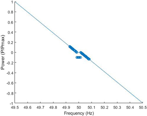
FIGURE 12. Power-frequency plots, demonstrating the VCS response to frequency events originating from historical data.

The variations in power and frequency throughout the experiment are depicted in the time series plot of Figure 13. The VCS reacts to the changes in frequency, with negative values of power indicating power absorption from the laboratory network and the positive value indicating power injection into the laboratory network. These correspond, respectively, to the operation of the electrolyser and the fuel cells. This figure also shows how LoH in the buffer changes during the experiment, with the electrolyser increasing the LoH in the buffer while the fuel cells decrease the LoH in the buffer.

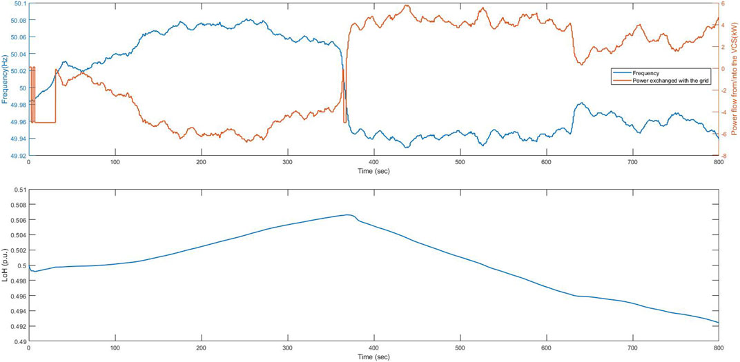
FIGURE 13. Plots of frequency, power and LoH against time, where the hydrogen buffer was at 50% of its capacity at the beginning of the its operation.

Figure 14 shows the input power to the electrolyser and the output power from the fuel cells during this experiment. These powers are calculated in the model deployed in the controller of the power source (VCS emulator) shown in Figure 9. These values match the values of the power exchanged with the laboratory network shown in Figure 13. Figure 14 also shows the amount of hydrogen, estimated in kW, consumed by the fuel cells and produced by the electrolyser. This figure shows that the efficiencies of the electrolyser and the fuel cell stacks are respectively 80% and 40%. The efficiency of the electrolyser has been calculated by dividing the amount of hydrogen produced by the electrolyser, in kW, by the input power to the electrolyser. In the same way, the efficiency of the fuel cell stacks was calculated by dividing their output power by the amount of hydrogen consumed by the fuel cells in kW. However, the overall efficiency of the VCS during the experiment was 55.4%. This value was calculated as follows:

where E_inj represents the energy injected to the grid estimated in kWh; E_con represents the energy consumed from the grid estimated in kWh; and ΔLoH is the change in hydrogen stored in the buffer estimated in kWh.

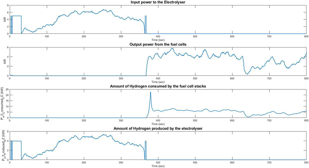
FIGURE 14. Plots of input power to the electrolyser, the output power from the fuel cells, the amount during their response to the frequency events originating from historical data.

The measured power and the power set point calculated from the measured frequency were cross-correlated (Knapp and Carter, 1976) to determine the response time of the VCS system. When the maximum correlation occurred, the response times were 2.857 s (Figure 15A) during under-frequency periods, corresponding to the operation of the fuel cells, and 2.252 s (Figure 15B) during over-frequency periods corresponding to electrolyser operation; this is within the range of the 10-s response time needed by the PFR standards.

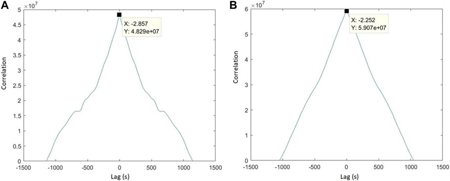
FIGURE 15. A plot demonstrating the cross-correlation between the measured power and the power set-point estimated from the measured frequency in two cases: (A) under frequency case when the fuel cells were in operation, (B) over frequency case when the electrolyser was in operation.

As shown in paragraph 2.1.4, the electrolyser model realistically reproduces the response produced by an actual electrolyser (Tuinema et al., 2020). The simulation results show that the maximum time delay is 2.25199 s. This delay represents the maximum time delay when the electrolyser was not interfaced with a power converter. Figure 15B shows the maximum time delay of the VCS during the period of over-frequency (the period during which the electrolyser is working) is 2.252 s. This means that there is a delay of 10 μs, and it corresponds to the delay of the power converter response.

4.2 Closed loop response to emulated frequency events

The response of the VCS during an emulated frequency event is illustrated in Figure 16, which includes the variation of system frequency and power response of the VCS. In the power system model, an imbalance between generation and demand has been considered. This imbalance corresponds to the case of loss of the maximum infeed generator, 1200 MW when the demand was 30 GW, which corresponds to the average demand in GB in 2019. This created a frequency drop. The VCS emulator in the laboratory observed a change in frequency and dispatched a power injection based on the control algorithm shown in Figure 7. Subsequent runs of the experiment involved applying various scaling factors to the VCS, corresponding to peak output levels of 300 MW, 600 MW, and 1200 MW, respectively. When the size of the VCS was increased, the frequency event was less severe. The VCS with the 600 MW and 1200 MW capacities were able to restore the nominal values of the system, however, the VCS with 300 MW brought the system frequency to 49.981 HZ which is within the statutory limit (±0.5 Hz) but not within the deadband (±0.015 Hz). The frequency nadir for each VCS capacity used within the experiments is shown in Figure 17. Also shown is the base case, which excludes VCS. It is important to highlight that the operation of the whole system, depicted in Figure 8, is stable and this can be explained as follows: the evolution of the frequency deviation in the power system model as a result of a step change in the input signal (ΔP_loss) is the step response of a first-order function controlled in a closed loop by a PID controller. Increasing the power set-point of the VCS corresponds to increasing the proportional action of the PID controller. Increasing the proportional action, in general, decreases the steady-state error (i.e., enhances the system accuracy).

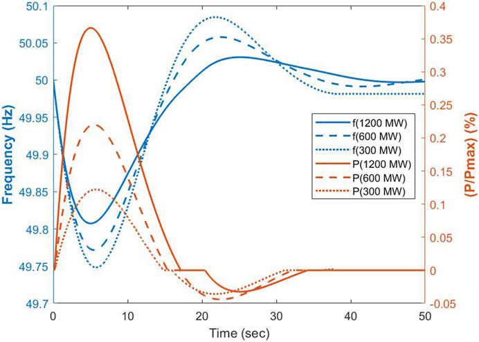
FIGURE 16. System frequency and the VCS responses for VCS ratings of 300–1200 MW.

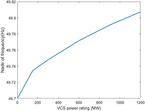
FIGURE 17. Nadir of frequency for the different power rating of the VCS.

4.3 Discussion

The following section aims to answer the research questions that were presented in Section 1, as well as explore potential directions for future research that could build on the methodology and results that were presented in this paper.

Results from analysing historical data show that there is a delay of around 2 s between the frequency crossing the threshold and the power being provided. This implies that a VCS can provide existing PFR services, but may not be suitable for emerging services which require a subsecond response. The experiments show that the VCS can manage the LoH in the hydrogen buffer while still delivering the service. In addition, the experiments enabled the evaluation of the efficiency of the VCS, which was 55.4%. This efficiency is affected by the low efficiencies of the electrolysis and fuel cell stacks. However, electrolyser and fuel cell manufacturers are striving to improve the efficiency of their equipment, and this will enhance the efficiency of the VCS.

The PHIL experiments demonstrated that providing PFR service through the VCS can mitigate the impact of a high-frequency event by lowering the most extreme deviations from the nominal frequency. Furthermore, as more VCS capacity was installed, the nadir frequency improved, although these improvements were greatest for the smallest VCS considered, indicating diminishing returns for the larger systems. The diminishing return is due to the design of the droop controller—as the nadir of frequency is reduced, the response required from the VCS is also reduced, so a smaller proportion of its greater capacity is actually mobilised. For example, with a nadir of frequency of 49.725 Hz and a 100 MW VCS, we would deliver a peak power of 100 MW. With a 500 MW VCS, we may only have a frequency nadir of 49.76, which would result in 350 MW being actually delivered; hence each additional MW of response will deliver a smaller improvement in the nadir of frequency because that additional MW is not fully utilized due to the smaller frequency deviation.

This paper’s methods and findings can address the research questions posed in the introduction and provide a foundation for future research. The techniques employed in this study may be utilized to examine the effectiveness of fast-responding, distributed VCS configurations. However, the necessary communications in a distributed configuration of electrolysers and fuel cells will cause additional latencies. These latencies might make this configuration more appropriate to provide secondary frequency response service where the required time response is in order of 30 s which can be met.

5 Conclusion

In order to reduce CO₂ emissions from power and energy systems, low-carbon technologies must form the backbone of these systems in the future. In this context, green hydrogen technologies such as electrolysers and fuel cells are of increasing interest. The research conducted in this paper has showed the potential and capacity of bidirectional vector coupling storage (VCS) that relies on hydrogen to offer frequency response services in forthcoming power systems. The paper presents a dynamic model of bi-directional VCS and introduces a comprehensive evaluation method that leverages digital twin and PHIL to assess the impact of VCS on the integrated energy system. Moreover, the paper demonstrates the viability of utilizing this storage for frequency response. The two experiments conducted in this paper illustrate the capacity of VCS to offer a genuine power response to transient events observed in the GB transmission network or induced by the GB power system model. The results of the experiments indicate that the response time of VCS is sufficiently fast to provide primary frequency response and that the VCS size has a significant impact on ensuring that the frequency remains within the statutory acceptable range of [49.5, 50.5] Hz.

It is important to highlight that the aim of this paper is not to compare the performance of VCS with other storage facilities providing the frequency response; the aim is to evaluate the technical feasibility of the VCS to offer a frequency response. Our future works include the techno-economic evaluation of the VCS offering primary frequency response and comparison of these evaluation parameters with those of other storage facilities.

Data availability statement

The original contributions presented in the study are included in the article/Supplementary material, further inquiries can be directed to the corresponding author.

Author contributions

AA: conceptualization, methodology, software, investigation, writing- original draft preparation. DG: conceptualization, methodology, investigation, reviewing and editing. CP: conceptualization, reviewing and editing. SW: supervision, funding acquisition. PT: conceptualization, reviewing and editing, funding acquisition. All authors contributed to the article and approved the submitted version.

Funding

The research presented in this paper is a part of the United Kingdom EPSRC-funded project titled “Supergen Energy Networks Hub” with the reference number “EP/Y016114/1”.

Acknowledgments

More information on the project can be found at “https://www.ncl.ac.uk/supergenenhub/”.

Conflict of interest

The authors declare that the research was conducted in the absence of any commercial or financial relationships that could be construed as a potential conflict of interest.

Publisher’s note

All claims expressed in this article are solely those of the authors and do not necessarily represent those of their affiliated organizations, or those of the publisher, the editors and the reviewers. Any product that may be evaluated in this article, or claim that may be made by its manufacturer, is not guaranteed or endorsed by the publisher.

References

Abeysekera, M., Jenkins, N., and Wu, J. (2016). Integrated energy systems: An overview of benefits, analysis, research gaps and opportunities.
Alexander, B., and Spliethoff, H. (2018). Current status of water electrolysis for energy storage, grid balancing and sector coupling via power-to-gas and power-to-liquids: A review. Renew. Sustain. Energy Rev.82, 2440–2454. doi:10.1016/j.rser.2017.09.003
Alshehri, F., Suárez, V. G., Torres, J. L. R., Perilla, A., and van der Meijden, M. (2019). Modelling and evaluation of pem hydrogen technologies for frequency ancillary services in future multi-energy sustainable power systems. Heliyon5 (4), e01396. doi:10.1016/j.heliyon.2019.e01396
Amphlett, J. C., Mann, R. F., Peppley, B. A., Roberge, P. R., and Rodrigues, A. (1996). A model predicting transient responses of proton exchange membrane fuel cells. J. Power sources61 (1-2), 183–188. doi:10.1016/s0378-7753(96)02360-9
Andújar, J. M., Segura, F., and Vasallo, M. J. (2008). A suitable model plant for control of the set fuel cell-dc/dc converter. Renew. Energy33 (4), 813–826. doi:10.1016/j.renene.2007.04.013
Aupetit, S., and Pokluda, M. (2018). System protection behaviour and settings during system disturbances. Rev. Rep. Eur. Netw. Transm. Syst. Operators Electr. (ENTSO-E). Tech. Rep.
Australian Energy Market Operator (2019). Final report-queensland and south Australia system separation on 25 august 2018. Australia: AEMO Information & Support Hub, Tech. Rep.
Australian Energy Market Operator (2016). Response of existing pv inverters to frequency disturbances. Australia: AEMO Information & Support Hub.
Banks, J., Bruce, A., and MacGill, I. (2017). “Fast frequency response markets for high renewable energy penetrations in the future Australian nem,” in Proceedings of the asia pacific solar research conference.
Bian, Y., Wang, H., Wyman-Pain, H., Gu, C., and Li, F. (2017). Frequency response in the gb power system from responsive chps. Energy Procedia105, 2302–2309. doi:10.1016/j.egypro.2017.03.664
Borth, M., Verriet, J., and Muller, G. (2019). “Digital twin strategies for sos 4 challenges and 4 architecture setups for digital twins of sos,” in 2019 14th annual conference system of systems engineering (SoSE) (IEEE), 164–169.
Cheng, M., Wu, J., Galsworthy, S. J., Ugalde-Loo, C. E., Gargov, N., Hung, W. W., et al. (2015). Power system frequency response from the control of bitumen tanks. IEEE Trans. Power Syst.31 (3), 1769–1778. doi:10.1109/tpwrs.2015.2440336
Clegg, S., and Mancarella, P. (2015). Integrated electrical and gas network flexibility assessment in low-carbon multi-energy systems. IEEE Trans. Sustain. Energy7 (2), 718–731. doi:10.1109/tste.2015.2497329
Ghazavi Dozein, M., Jalali, A., and Mancarella, P. (2021). Fast frequency response from utility-scale hydrogen electrolyzers. IEEE Trans. Sustain. Energy12, 1707–1717. doi:10.1109/tste.2021.3063245
Ghazavi Dozein, M., and Mancarella, P. (2019). “Application of utility-connected battery energy storage system for integrated dynamic services,” in 2019 IEEE milan PowerTech (IEEE), 1–6.
Greenwood, D. M., Lim, K. Y., Patsios, C., Lyons, P. F., Lim, Y. S., and Taylor, P. C. (2017). Frequency response services designed for energy storage. Appl. Energy203, 115–127. doi:10.1016/j.apenergy.2017.06.046
Grigsby, L. L. (2007). Power system stability and control. Boca Raton: CRC Press. Available at: https://www.taylorfrancis.com/books/edit/10.4324/b12113/power-system-stability-control-leonard-grigsby
Guillaud, X., Omar Faruque, M., Alexandre, T., Hariri, A. H., Vanfretti, L., Paolone, M., et al. (2015). Applications of real-time simulation technologies in power and energy systems. IEEE Power Energy Technol. Syst. J.2 (3), 103–115. doi:10.1109/jpets.2015.2445296
HM Government (2023). Carbon budget delivery plan. Available at: https://assets.publishing.service.gov.uk/government/uploads/system/uplo ads/attachment_data/file/1147369/carbon-budget-delivery-plan.pdf.
Hou, Y., Yang, Z., and Wan, G. (2010). An improved dynamic voltage model of pem fuel cell stack. Int. J. hydrogen energy35 (20), 11154–11160. doi:10.1016/j.ijhydene.2010.07.036
Knapp, C., and Carter, G. (1976). The generalized correlation method for estimation of time delay. IEEE Trans. Acoust. speech, signal Process.24 (4), 320–327. doi:10.1109/tassp.1976.1162830
Kong, X., Khambadkone, A. M., and Thum, S. K. (2005). A hybrid model with combined steady-state and dynamic characteristics of pemfc fuel cell stack. In Fourtieth IAS annual meeting. Conference record of the 2005 industry applications conference3, 1618–1625. IEEE.
Miland, H. (2005). Operational experience and control strategies for a stand-alone power system based on renewable energy and hydrogen.
National Grid ESO (2023). The grid code. Available at: https://www.nationalgrideso.com/document/162271/download.
National Grid, ESO (2019). Future energy scenarios. London, UK: National Grid Electricity System Operator, 1–166.
Nguyen, V. H., Tran, Q. T., Besanger, Y., Jung, M., and Nguyen, T. L. (2022). Digital twin integrated power-hardware-in-the-loop for the assessment of distributed renewable energy resources. Electr. Eng.104 (2), 377–388. doi:10.1007/s00202-021-01246-0
Nikiforow, K., Pennanen, J., Ihonen, J., Uski, S., and Koski, P. (2018). Power ramp rate capabilities of a 5 kw proton exchange membrane fuel cell system with discrete ejector control. J. Power Sources381, 30–37. doi:10.1016/j.jpowsour.2018.01.090
Restrepo, C., Konjedic, T., Garces, A., Calvente, J., and Giral, R. (2014). Identification of a proton-exchange membrane fuel cell’s model parameters by means of an evolution strategy. IEEE Trans. Industrial Inf.11 (2), 548–559. doi:10.1109/tii.2014.2317982
Reza Hosseini, S. H., Allahham, A., and Taylor, P. (2018). “Techno-economic-environmental analysis of integrated operation of gas and electricity networks,” in 2018 IEEE international symposium on circuits and systems (ISCAS) (IEEE), 1–5.
Reza Hosseini, S. H., Allahham, A., Walker, S. L., and Taylor, P. (2020). Optimal planning and operation of multi-vector energy networks: A systematic review. Renew. Sustain. Energy Rev.133, 110216. doi:10.1016/j.rser.2020.110216
Reza Hosseini, S. H., Allahham, A., Walker, S. L., and Taylor, P. (2021). Uncertainty analysis of the impact of increasing levels of gas and electricity network integration and storage on techno-economic-environmental performance. Energy222, 2021, 119968. doi:10.1016/j.energy.2021.119968
Saedi, I., Mhanna, S., Wang, H., and Mancarella, P. “Integrated electricity and gas systems modelling: Assessing the impacts of electrification of residential heating in victoria,” in 2020 australasian universities power engineering conference (AUPEC) (IEEE), 1–6.
Samarakoon, K., Ekanayake, J., and Jenkins, N. (2011). Investigation of domestic load control to provide primary frequency response using smart meters. IEEE Trans. Smart Grid3 (1), 282–292. doi:10.1109/tsg.2011.2173219
San Martín, I., Ursúa, A., and Sanchis, P. (2014). Modelling of pem fuel cell performance: Steady-state and dynamic experimental validation. Energies7 (2), 670–700. doi:10.3390/en7020670
Sarrias-Mena, R., Fernández-Ramírez, L. M., García-Vázquez, C. A., and Jurado, F. (2015). Electrolyzer models for hydrogen production from wind energy systems. Int. J. Hydrogen Energy40 (7), 2927–2938. doi:10.1016/j.ijhydene.2014.12.125
Sayfutdinov, T., Lyons, P., and Feeney, M. (2016). Laboratory evaluation of a deterministic optimal power flow algorithm using power hardware in the loop. CIRED Workshop2016, 1–4. doi:10.1049/cp.2016.0675
Soltani, M., and Taghi Bathaee, S. M. (2010). Development of an empirical dynamic model for a nexa pem fuel cell power module. Energy Convers. Manag.51 (12), 2492–2500. doi:10.1016/j.enconman.2010.05.012
Troncoso, E., and Newborough, M. (2011). Electrolysers for mitigating wind curtailment and producing ‘green’merchant hydrogen. Int. J. hydrogen energy36 (1), 120–134. doi:10.1016/j.ijhydene.2010.10.047
Tuinema, B. W., Adabi, E., Ayivor, P. K. S., Suárez, V. G., Liu, L., Perilla, A., et al. (2020). Modelling of large-sized electrolysers for real-time simulation and study of the possibility of frequency support by electrolysers. IET Generation, Transm. Distribution14 (10), 1985–1992. doi:10.1049/iet-gtd.2019.1364
Ursúa, A., San Martín, I., Barrios, E. L., and Sanchis, P. (2013). Stand-alone operation of an alkaline water electrolyser fed by wind and photovoltaic systems. Int. J. Hydrogen Energy38 (35), 14952–14967. doi:10.1016/j.ijhydene.2013.09.085
Wang, C., Hashem Nehrir, M., and Shaw, S. R. (2005). Dynamic models and model validation for pem fuel cells using electrical circuits. IEEE Trans. energy Convers.20 (2), 442–451. doi:10.1109/tec.2004.842357
Werner, K., Karner, M., Traar, G., Jan, H., and Sihn, W. (2018). Digital twin in manufacturing: A categorical literature review and classification. IFAC-PapersOnLine51 (11), 1016–1022. doi:10.1016/j.ifacol.2018.08.474
Keywords: smart grid, digital twin, power-hardware-in-loop (PHIL) simulation, frequency response, electrolyser model, fuel cell modeling
Citation: Allahham A, Greenwood D, Patsios C, Walker SL and Taylor P (2023) Primary frequency response from hydrogen-based bidirectional vector coupling storage: modelling and demonstration using power-hardware-in-the-loop simulation. Front. Energy Res. 11:1217070. doi: 10.3389/fenrg.2023.1217070
Received: 04 May 2023; Accepted: 30 June 2023;
Published: 19 July 2023.
Edited by:
Kenneth E. Okedu, Nişantaşı University, TürkiyeReviewed by:
Hind Barghash, German University of Technology in Oman, OmanKui Luo, China Electric Power Research Institute (CEPRI), China
Copyright © 2023 Allahham, Greenwood, Patsios, Walker and Taylor. This is an open-access article distributed under the terms of the Creative Commons Attribution License (CC BY). The use, distribution or reproduction in other forums is permitted, provided the original author(s) and the copyright owner(s) are credited and that the original publication in this journal is cited, in accordance with accepted academic practice. No use, distribution or reproduction is permitted which does not comply with these terms.
*Correspondence: Adib Allahham, adib.allahham@northumbria.ac.uk