Reduced order modeling of non-linear monopile dynamics via an AE-LSTM scheme

1 Introduction

Wind energy plays an increasingly vital role in global power production; however, its success largely relies in the associated reduction of the levelised cost of energy of wind farms. These price improvements can be associated with the use of increasingly large turbines and advanced materials, as well as the extended use of offshore wind resources, which prove potent and more consistent University of Michigan. (2021); Sadorksy (2021). The complex nature of wind energy structures and, the adverse operational environments to which these are exposed, require accurate analysis tools for the simulation of their dynamic behaviour. Such dynamic models are important both during the design phase, for estimating and accounting for expected loads and displacements, as well as during operation for the purpose of health monitoring and remaining life prediction Tatsis et al. (2017); Hu et al. (2015a,b); Devriendt et al. (2014); Martinez-Luengo et al. (2016). In order to achieve sufficient fidelity, the employed dynamic models should further account for presence of non-linear effects Wagg et al. (2020); Pimenta et al. (2020).

A considerable source of non-linearity in wind turbine structures stems from the Soil Structure Interaction (SSI) effect Abdullahi et al. (2020); Zuo et al. (2018); Abhinav and Saha (2018). In offshore installations the turbines are anchored to the ground using a monopile foundation driven into soil. The monopile interaction with the soil is governed by SSI effects. Soils are known to comprise considerably non-linear behaviour exhibiting softening and non-linear damping Jardine et al. (1986). SSI phenomena affect the wind turbine’s dynamic response and, as such, need to be adequately accounted for Abdullahi et al. (2020); Harte et al. (2012). The required non-linear analyses imply a severe increase in computational complexity, which often renders such a task impractical. This is particularly true for computing tasks which require repeated or multiple evaluations, such as uncertainty quantification Sudret et al. (2017), model updating Rogers et al. (2019); Cao et al. (2020), or digital twinning Solman et al. (2022). The concept of digital twinning is particularly appealing for offshore assets, where frequent inspection is costly or infeasible. In the context of structural monitoring, digital twins imply interaction with a digital counterpart, i.e., a model of the system which ought to be computationally efficient, so that data may be assimilated feasibly on the fly. This motivates the use of Reduced Order Models (ROMs) for computationally intensive tasks, such as non-linear simulations related to the SSI problem.

The majority of established ROM techniques are intended for linear systems, and are largely pertaining to projection-based methods in which the equations of motion are projected onto a lower dimensional subspace hence reducing the dimensionality of the problem and allowing a faster solution Craig and Kurdila (2006). For dynamic systems, these subspaces usually correspond to mode shapes of the system, which can be extracted through the eigendecomposition of the structural matrices. Instances of such methods, such as the Craig-Bampton Craig and Bampton (1968) and modal superposition methods Craig and Kurdila (2006) are widely implemented in finite element (FE) software Smith (2009); Ansys-Inc (2013) and can significantly reduce the computational effort of linear calculations, whilst maintaining high fidelity. The presence of non-linearity in a system, however, will cause such methods to lose efficiency or fail. This motivates the use of non-linear reduction schemes. Some of these methods retain the philosophy of the linear methods, for instance by exploiting analytically extracted mode shape bases and enriching these with higher order terms of the Taylor approximation (modal derivative vectors), which can allow for capturing a certain amount of non-linearity Wu and Tiso (2016); Tatsis et al. (2018). Alternatively, an established approach to non-linear reduction refers to adoption of Proper Orthogonal Decomposition (POD) schemes Carlberg and Farhat (2008); Chinesta et al. (2011); Farhat et al. (2014). POD methods use ‘snapshots’ of output data from Full Order simulations carried out on the system of interest. A singular value decomposition of the response of the system in these snapshots is then carried out in order to empirically find a suitable linear subspace, which approximates the solution. These methods are powerful, especially when combined with hyper-reduction techniques Vlachas et al. (2021), but can become inefficient with regards to the required size of the projection basis for systems with strong non-linearities. To alleviate this issue, POD bases are typically parameterised in terms of the system characteristics or input (excitation) properties Amsallem and Farhat (2008); Vlachas K. et al. (2022).

A separate approach pertains to reduction on a lower dimensional non-linear manifold, which targets a more compressed (reduced) latent space at similar levels of accuracy Lee and Carlberg (2020); Cenedese et al. (2022); Jain et al. (2017). In this work, we make use of a recently developed non-linear ROM framework Simpson et al. (2021) which employs such a non-linear reduction. The method makes use of an AutoEncoder (AE) neural network, which is combined with a Long Short-Term Memory (LSTM) neural network, which represents the dynamics in the reduced space. A similar methodology has been developed by Vlachas et al. Vlachas P. R. et al. (2022) applied to dynamic problems in more wide ranging scientific disciplines. The AE reduction is purely based on input and output data from training simulations taken from the full order model (FOM), while no information from structural matrices or the nature of non-linearities are required, since the numerical integration is executed by the LSTM and not a reduced physics equation. Having trained the ROM, the system response can be approximated for new forcing input time histories much more rapidly than carrying out the same simulations using the FOM.

In this work the ROM is tailored to the SSI problem characterizing the interaction an offshore wind turbine monopile with soil. The SSI problem is considered in isolation from the aeroelastic turbine model; however, the input forces used at the boundary of the monopile are taken from a coupled SSI-Aeroelastic simulation and can hence be considered representative for the purposes of training a ROM. A FOM of the system is created in collaboration with the Siemens Gamesa partners, using the Abaqus FE software. The monopile is modelled using linear beam elements, while the movement of the monopile is constrained by depth-dependent, non-linear spring and dashpot elements. The non-linear stiffness and damping relations of these elements is provided by Siemens Gamesa and aim to reflect a representative North Sea project. Input forcing and moments are applied to the top-most node of the monopile at the “mud line”, and are, as previously mentioned, extracted from full order coupled simulations. Time histories are used from 75 different loading conditions at varying wind speed and wave intensities. Corresponding FOM simulations were carried out for each of the 75 parametric configurations and 6 of these are used to train the ROM. The trained ROM is then tested on the remaining 69 FOM simulations that have not been included in the training dataset and the performance of the ROM is evaluated by comparing the fidelity to the FOM response and the reduction in computational time achieved.

The layout of this paper is as follows: Section 2 describes the SSI phenomenon and its relevance to wind energy structures, as well as the specific assumptions assumed herein for simulation of the SSI effect. Section 3 offers background on ROM methodologies as well as detailing the ROM method used herein and its constituent algorithms. Section 4 details the data generation from the FOM, which is then used for training and testing of the ROM. Section 5 then presents the process of training the ROM, as well as the final architectures of the neural networks used. Section 6 presents the results of the ROM testing and reports on the precision achieved with respect to the FOM simulations as well as on the attained reduction in computational time. Finally, Section 7 concludes the paper by summarising the work and results achieved and offering perspectives on future developments.

2 Soil structure interaction in wind turbines

Soil structure interaction is a complex area of research at the intersection of soil mechanics and structural mechanics. The study of SSI was principally driven from the desire to increase the seismic performance of structures and for offshore engineering Matlock and Reese (1960); Wong (1975). SSI has traditionally been regarded as beneficial to structural response as a result of adding damping and lengthening the oscillation periods Mylonakis and Gazetas (2000); Martakis et al. (2017). In the context of earthquake engineering, it was thus previously recommended to ignore these effects, considering this as an additional margin for safety. However, when considering dynamically complex structures, such as wind turbines, this assumption does not always hold Harte et al. (2012), implying that if high precision is desired in terms of twinning applications, such effects must be accounted for.

Available simulation methods for SSI effects span from simplified schemes, such as use of linear rotational, horizontal and vertical springs Adhikari and Bhattacharya (2011), to numerically demanding schemes, where the soil is modelled as a non-linear continuum via FE methods Cao et al. (2020). The most basic models may be sufficient to capture SSI-induced shifts in natural frequencies, however, more refined FE models are necessary to represent the full non-linear, hysteretic response of the soil. A commonly used method, which represents a middle ground amongst available schemes, is the P-Y curve method Wolf et al. (2013); Pando et al. (2006). The P-Y curve method was originally developed in the 1970s for treating long piles driven into offshore soils Matlock (1970). The method substitutes the soil with multiple non-linear spring elements with depth-dependent behaviour. The non-linear springs may also be supplemented by non-linear damping elements, which can be depth-dependent. The P-Y curve method does not take into account the hysteretic behaviour of soil as is suggested in some relevant literature Whyte et al. (2020), but does capture the strong strain-softening non-linear behaviour observed in most soils. The non-linear springs are usually defined using empirical relations dependent upon various properties of the specific soil type considered or by calibration with FE models. The P-Y curve is broadly adopted in the wind energy domain, both in research Sajeer et al. (2021) and relevant industry standards DNV (2014). In this work, motivated by current practice, the P-Y curve method is implemented within a finite element FOM setting of which a ROM is to be constructed. Whilst such an implementation is not as computationally taxing as full continuum FE methods, it remains a significant computational hurdle in the simulation of coupled wind turbine/SSI systems.

We consider the SSI problem of an offshore wind turbine mounted on a monopile foundation in soil; the assumed system is shown in Figure 1. In this figure, the monopile and surrounding soil is considered as one sub-system, while everything above the mudline, namely, the wind turbine and the wave/wind loading as a separate sub-system. In our analysis we focus only on the modelling of the interaction effect between the monopile and surrounding soil, whilst the presence of the wind turbine is simulated, again following engineering practice, in the form of interface forces and moments applied to the monopile at the mudline. This allows to create a ROM of the SSI problem in isolation, which can be coupled to any existing model of the structure/system lying above the mudline. Such an approach necessitates that the force and moment time histories applied to the monopile at the mudline are representative of those that would be applied in a coupled simulation. To this end, these are extracted from coupled simulations which are performed based on a multi-megawatt turbine, where the FOM of the SSI utilises the PY curve method. Therefore, in the case where the ROM perfectly replicates the FOM, these interface forces would lead to an exact match of displacements and rotations.

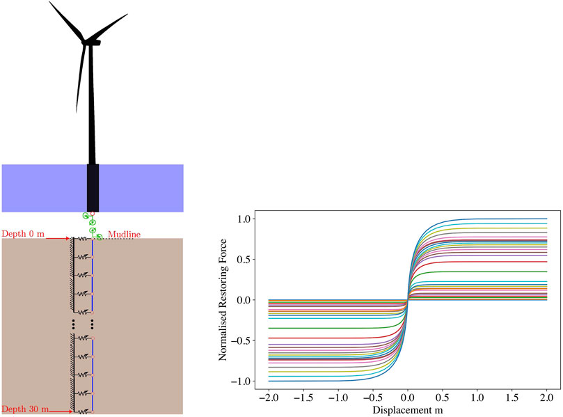
FIGURE 1. Left: Sketch of the modelled system, indicating the coupling between the wind turbine and soil through distributed non-linear spring forces. Right: Normalised non-linear restoring force-displacement (P–Y) curves of the soil at various depths in the y-axis.

The system to be modelled consists of a linear steel monopile constrained by soil exhibiting non-linear restoring force. The monopile is excited at the node at the top of the monopile at the mudline, through applied forces and moments which are extracted from coupled simulations. The dimensions and material of the monopile reflect representative values for modern offshore wind applications: the monopile has an outer diameter of 9.5 m, a wall thickness of 0.08 m and a length of 30 m with a constant annular cross section. The monopile is modelled with 31 nodes connected by 30 linear beam elements, whilst the restoring force of the soil is represented, as dictated by the P-Y curve method, by non-linear springs and non-linear dashpots constraining all 31 of the nodes in the x and y directions. The properties for these depth-dependent non-linear springs are provided by Siemens Gamesa and aim to reflect values corresponding to a representative North Sea project, and aim to reflect values of a representative North Sea project. The non-linear dashpot curves are approximated proportional to the stiffness at a ratio of 0.001 to the stiffness. The depth-dependent non-linear restoring force-displacement (P-Y) curves, representing the soil stiffness, are demonstrated in the right subplot of Figure 1.

75 different time histories of forcing and moments were extracted from coupled simulations. These correspond to parametric sets of 25 different wind and wave intensity levels varying from 3–28 m/s average wind speed. Each wind speed has a corresponding turbulence intensity as presented in the Supplementary Material, the wave loading was generated using a JONSWAP distribution Hasselmann et al. (1973) wherein the wave amplitude varies almost linearly from 0.2 to 7 m between 3 and 28 m/s. Three simulations are carried out at each distinct parametric configuration, with each simulation corresponding to a different random seed for generating the corresponding wind turbulence and wave loading. An example time history corresponding to 14 m/s is shown in Figure 2, which illustrates the forces (top subplots) and moments (bottom subplots), along the x (left subplots) and y directions (right subplots), acting on the monopile node at the mudline. The generated time series cover a total simulation time of 600 s, at a sampling period of 0.02 s.

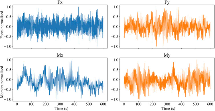
FIGURE 2. Sample input forcing (top) and bending moment (bottom) time histories at the mudline, along the x (left) and y (right) directions; directions are indicated in 1.

3 Reduced order modelling via AE-LSTM

The AE-LSTM ROM methodology used herein was recently developed by the authors Simpson et al. (2021) by coupling an AutoEncoder (AE) with LSTM neural networks. The autoencoder is employed for dimensionality reduction, while the LSTM reflects a recurrent neural network (RNN) for learning the underlying, possibly non-linear, dynamics. The method is a purely data based modelling method and has been shown to have significant capability for modelling the behaviour of strongly non-linear systems. The method has also been shown to be agnostic to the non-linearity type present, showing good performance with both a cubic type non-linearity and a Bouc-Wen hysteretic non-linearity Simpson et al. (2021). It is worth mentioning that when a VAE is adopted, in place of a plain AE, the latent space becomes statistically independent, implying that the underlying states resemble Non-linear Normal Modes (NNMs), as illustrated in Simpson et al. (2023); Champneys et al. (2022). While useful for decoupling the feature space in terms of carried spectral content, this approximation is not necessary for the ROM construction. In this work we extend the AE-LSTM methodology to deal with a realistic system, which represents a real issue faced by the industry in offshore wind energy systems.

3.1 Autoencoder neural networks

An autoencoder neural network is a type of neural network typically used for dimensionality reduction or de-noising applications Hinton and Salakhutdinov (2006). They are a type of Deep Neural Network (DNN) assuming a specific vector input, which is reproduced (decoded) as output, whilst the architecture of the network forces (encodes) this vector through a low dimensional “bottleneck layer”. This requires that the network learn a non-linear transform to a lower dimensional space which retains maximal information, such that the vector can be optimally reconstructed from this lower dimensional representation. The trained AE then contains both an encoder, which can transform data to the reduced space, and a decoder, which performs the opposite operation, returning from the compressed to the physical space. The architecture of an autoencoder is demonstrated in Figure 3, in this case we see an autoencoder with a 4 dimensional input vector X and a 2 dimensional bottleneck layer Z. The autoencoder outputs an approximation of the input vector $\tilde{X}$.

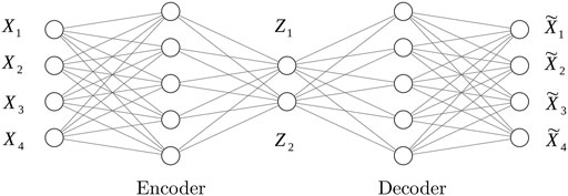
FIGURE 3. Diagram of an autoencoder neural network featuring 4 dimensional input/output and 2 dimensional hidden layer.

Autoencoders are very often used in machine learning applications as an unsupervised learning scheme for efficient feature extraction Vincent et al. (2008). Feature extraction is a common operation in machine learning methods and involves transformation of data to render these more efficient for use with downstream machine learning tasks. Successful feature extraction relies on reducing the dimensionality of the data Hinton and Salakhutdinov (2006). Autoencoders are part of a group of methods known as manifold learning algorithms, which target extraction of structure from datasets in an unsupervised manner Izenman (2012). The most widely known and essential of such methods is Principal Component Analysis (PCA). PCA seeks the optimal orthogonal projection of a dataset onto a reduced number of dimensions, whilst preserving the maximum possible variance Wold et al. (1987). An interesting detail in the domain of structural dynamics is that, for linear systems, implementation of PCA on the output response of a structural system is equivalent to operational modal analysis, and is equivalent to learning a transformation of the data to the modal domain Poncelet et al. (2007). Following this logic, when tackling non-linear systems, the use of a non-linear method can more efficiently extract such a reduced structure. Autoencoders are one such non-linear manifold learning method with certain advantages. Firstly, they efficiently scale to high dimensions. Secondly, they naturally provide both a forward and inverse transform from the physical to the reduced space. This is a very important aspect for ROMs within the context of SHM, as it allows reconstructing the system’s response in the physical coordinates, which represent the actually monitored space.

Autoencoders have found success in very diverse scientific fields, such as anomaly detection Sakurada and Yairi (2014), image processing and drug discovery. With regards to dynamical systems, autoencoders have been used in a number of cases where reduction on the basis of a manifold of lower dimension is deemed feasible Yoo et al. (2017). In Holden et al. Holden et al. (2015) autoencoders are used to capture a lower dimensional representation of videos of human motion. Lee and Carlberg Lee and Carlberg (2020) made use of convolutional autoencoders in conjunction with the non-linear Galerkin method to construct reduced order models. Vlachas et al. made use of autoencoders in combination with LSTM networks for modelling what they term the Learning of Effective Dynamics (LED) across multiple scales in areas of chemistry and fluid dynamics Vlachas P. R. et al. (2022). Lopez and Atzberger examine the use of variational autoencoders for uncovering lower dimensional dynamics in the Burgers equation Lopez and Atzberger (2020).

Regarding non-linear structural dynamics systems, a theory exists justifying the existence of such low dimensional manifolds, that is the theory of non-linear normal modes (NNMs) Kerschen et al. (2009). There further exists work connecting these NNMs with manifold learning techniques operated on output-only data; these refer to extraction using locally linear embedding Dervilis et al. (2019), generative adversarial networks Tsialiamanis et al. (2022) and variational autoencoders Simpson et al. (2023). Through these NNMs, parallels may also be drawn between autoencoders and structural dynamics, similarly to the relationship between PCA and linear modes. The connection comes in that, linear POD methods have been shown to find the best linear approximation of NNMs Kerschen et al. (2005) and further, that an autoencoder with linear activation functions will recreate the behaviour of POD Baldi and Hornik (1989). Such a connection to NNMs becomes more clear if we would consider the behaviour of a VAE Kingma and Welling (2014), in a VAE the latent space, which we consider to be approximating the NNMs, is encouraged to take the form of a given variational distribution, in most cases a diagonal Gaussian. This promotes statistical independence of the latent space variables and hence fulfils the NNM definition used by Worden and Green Worden and Green (2016).

3.2 LSTM neural networks

An LSTM neural network is a type of recurrent neural network (RNN), a neural network designed for modelling sequence data Rumelhart and McClelland (1987). RNN’s are conceptually similar to a non-linear auto-regressive with exogenous variable (NARX) model, which has been standardly adopted in dynamics and time series simulations CHEN and BILLINGS (1989). Similarly to NARX models RNNs deliver a prediction at time point t using predicted outputs at time point t − 1 and some exogenous variables from time point t. The key difference of the RNN to a NARX neural network, is that instead of explicitly using the predicted output of the model at previous time steps t − n - t − 1, where n is the number of lags in the NARX model, the internal state of the network at t − 1 is passed as endogenous input to time t. The passing of the internal state allows RNNs to achieve good predictive performance on sequence data whilst not being constrained to a certain pre-prescribed number of lags. The latter would limit the number of past values, which are assumed to influence the prediction, as would be the case for a traditional NARX model.

In practice, long term relations are difficult to learn by means of RNNs due to disappearing/exploding gradients during training. The LSTM network is a variation on a traditional RNN designed to combat this drawback, allowing for learning of long-term sequences. LSTM cells have been the key architecture for much of the successful uses of RNNs in recent years. The gated activation functions, which are key to LSTM networks, allow for improved capture of arbitrarily long relationships in sequence data. These have found applications in extensive fields, such as sequence modelling Bayer (2015), handwriting recognition Graves et al. (2007) and natural language translation Wu et al. (2016). Considerable success has been found in modelling dynamical systems of general nature, as well as structural systems in particular. In this context, Vlachas et al. Vlachas et al. (2018) consider the use of an LSTM network to model a chaotic Lorenz dynamic system. The use of LSTM networks has also been demonstrated for the reduced order modelling of non-linear aerodynamic simulations Wang and Wu (2020). Very recent work has also made use of physics informed LSTM networks to improve performance compared to purely data driven methods Zhang et al. (2020).

The LSTM cell is demonstrated in Figure 4 along with their defining parameters described in Eq. 1. The values i_t, f_t, o_t are the gates signals, of the forget, input and, output gates respectively. X_t, h_t−1, C_t−1 are the exogenous input, and the hidden and cell state from the previous time step whilst Uⁱ, U^f, U⁰, Wⁱ, W^f, W⁰ are weight matrices. The activation function σ is a sigmoid function. The full description and function of these equations can be found in the literature Hochreiter and Schmidhuber (1997) but the key element to the LSTM is the cell state C_t−1, this is the vector which is passed between time steps akin to the auto-regressive vector in a NARX model. This cell state acts as the memory of the network and the key difference is rather than the values in this vector being changed at every time step, to the previous network output, the values in the vector default to remaining the same. How this cell state is updated is controlled by the 3 “gates”: the forget, the update and output gate. These gates are also learned during the training of the network, as such if it proves advantageous for values to remain in the cell state over long sequences then this will be learned, this kind of behaviour is much more difficult to learn in vanilla RNN models. It is as a result of these gate functions that the LSTM network proves resistant to vanishing and exploding gradients. Due to the gating functions, the gradient of the cell is no longer intrinsically driven towards zero as in standard RNNs preventing vanishing gradients. Furthermore, the gradient of the cell state is upper bounded by 1 preventing exploding gradients Bayer (2015).

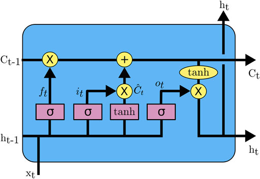
FIGURE 4. Architecture of the LSTM network cell: the previous output of the network h_t−1 is concatenated with the exogenous input x_t, the forget the update and output gates then define how this vector interacts with the cell state of the network C_t−1 to then given the new cell state C_t and network output h_t.

3.3 AE-LSTM ROM

The overall process of the ROM framework is illustrated in Figure 5. The ROM framework has two stages; the training stage, on the basis of input/output data from FOM simulations, and the testing stage, in which new (previously unseen) input time series are used by the ROM to generate predicted outputs. The upper subplot of Figure 5 demonstrates the training step of the ROM. Given that input, output data have already been generated from the FOM of the system of concern. The first step adopts output-only data from the FOM simulations, e.g., time-series of the displacement response at all monitored DOFs, and uses this to train an autoencoder to reduce the dimensionality of the data. The x and y displacement and R_x and R_y rotation time histories at each of the 31 nodes of the FE model, is aggregated in matrix [X]. The autoencoder then determines a non-linear transform, which reduces the 124 DOFs to a reduced space of dimension n, of latent variables represented in vector [Z]. The reduced dimension is considerably smaller than the original 124 DOFs and is selected so as to balance the amount of dimensionality reduction against the decrease in fidelity of said reduction. Simultaneously, the autoencoder learns the inverse operation; a non-linear transform, which returns from the reduced latent space [Z] to the approximated physical DOFs $[\tilde{X}]$.

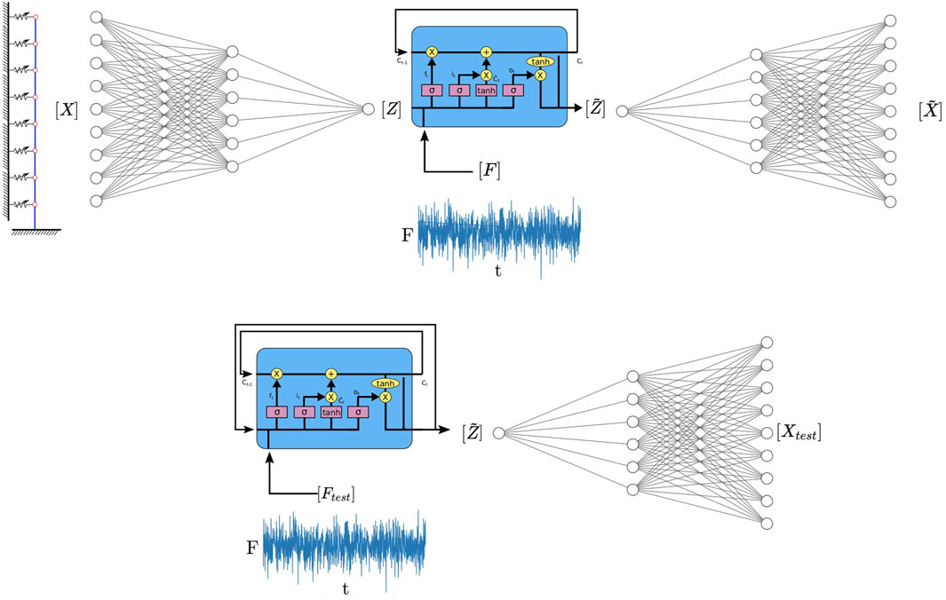
FIGURE 5. Upper: AE-LSTM based ROM framework in training mode, the AE is trained to transform the response vector X to the latent vector Z and the inverse transform of Z to $\tilde{X}$ whilst the LSTM is trained to predict $\tilde{Z}$ from the forcing time series F. Lower: AE-LSTM based ROM framework in testing mode. The LSTM network directly predicts the response in the latent space $\tilde{Z}$ to a new forcing time series F_test and the decoder reconstructs the response prediction in the physical space $\tilde{X}$.

Upon training of the autoencoder, the LSTM network must then be trained to learn the system dynamics. The LSTM network is trained using the force/moment time series as inputs and outputs the time series of the response in the reduced (latent) space of the n dimensions of the autoencoder bottleneck layer. As indicated in the upper subplot of Figure 5, the LSTM network learns to predict the latent space response of the system $[\tilde{Z}]$, taking as exogenous input the forcing time series collected in matrix [F] as well as the predicted output from the previous time step ${\tilde{Z}}_{t-1}$.

Having trained both the autoencoder and LSTM networks, the AE-LSTM ROM can then be used in prediction mode for predicting the response of the system to new forcing time histories. The testing stage of the ROM is shown in the lower subplot of Figure 5. The LSTM network admits a new set of forcing/moment time histories as inputs [F_test], and outputs the predicted response of the system in the reduced dimensional latent space $[\tilde{Z}]$. The predicted response in the original physical coordinates is then recreated by passing $[\tilde{Z}]$ through the decoder portion of the autoencoder to find the predicted response $[\tilde{X}]$. Prediction takes place in the reduced coordinate space which results in a lightweight and easily trainable model. The full methodology is more deeply examined and described in Simpson et al. (2021).

4 Data generation

In order to train and test the ROM, FOM simulations are executed for the 75 input time series, 6 of which will be used to train the ROM and the remaining 69 for testing its performance. The FOM as previously described in section 2, was created in Abaqus FE software Smith (2009); the Abaqus implicit solver was then used to simulate the dynamic response of the monopile SSI problem, with each simulation lasting 600 s with a maximum step size of 0.02 s. The response vectors were interpolated onto a constant sampling time of 0.02 s, as the Abaqus solver uses a varying time step integration scheme. Following the FOM simulations, the data was prepared for training the ROM. Firstly, the DOFs to be captured by the ROM were selected, the chosen DOFs were those normally of interest to Siemens Gamesa in their simulations. The DOFs of interest were defined as the x and y displacements and r_x and r_y rotations at each of the 31 nodes of the monopile. This results in 124 DOFs to be monitored.

Figure 6 plots the restoring force against displacement for one of the simulations carried out at 14 m/s wind speed. The response curve reveals significant non-linear behaviour. It is noteworthy that the restoring force plot is not symmetrical; this is due to non-zero mean forcing being applied to the system during the simulations.

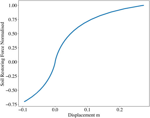
FIGURE 6. Force displacement plot of the ROM simulated response at DOF 30, corresponding to the x displacement of the topmost node at 0 m depth, for a simulation carried out at 14 m/s, with clearly evident non-linear behaviour.

5 ROM training

In order to fairly test the performance of the ROM, the data must be separated into suitable training and testing sets. The training data should cover the expected range of parameters/conditions within which the ROM is intended to perform. Simultaneously, however, we wish to minimise the number of expensive FOM runs required to train the model, to minimize the amount of training data. Furthermore, we would like to check the extrapolation performance of the ROM, i.e., we want to test the performance of the ROM at wind speeds higher or lower than those contained in the training set. To this end, the training set is selected to contain 6 of the original 75 input time series, at wind speeds of 7, 10, 13, 16, 22, 25 m/s. The testing set spans wind speeds from 3–28 m/s, allowing to test the extrapolation qualities of the ROM for wind speeds below 7 and above 25 m/s.

5.1 Autoencoder training

The autoencoder is then trained to as closely as possible recreate the displacement/rotation time series, which serves as both input and output. To this end, a mean squared error cost function between the input and output vectors is used, as defined in Eq. 2.

where M denotes the number of DOFs in the system, N stands for the number of data points or time steps, X_i is the M dimensional true response vector at step i and $\widehat{X_i}$ is the approximated M dimensional response vector outputted by the autoencoder for the sample at step i. By reducing this cost function we teach the autoencoder to learn a non-linear transform to a low dimensional space, whilst optimally reconstructing the original vector from the reduced space. The autoencoder is trained using the ADAM optimisation algorithm Kingma and Ba (2015) using the 6 training data series. Each of these datasets consists of 600 s of simulation at 0.02 s sampling rate giving a total of 30,000 data points, corresponding to the standard coupled simulations currently carried out by Siemens Gamesa. As such, for training the autoencoder, a total of 180,000 data points were used.

A critical step in the reduction process pertains to selection of a suitable dimension of the bottleneck layer. In order to do this, autoencoders were trained with consistent architectures but for a varying dimension of the bottleneck layer. The left hand sub figure of Figure 7 shows the reconstruction error of these autoencoders plotted against the dimension of the latent space. The error initially decreases significantly with increasing dimension, however, it plateaus for a dimension size larger than 4. Since we want to achieve maximum reduction whilst maintaining good fidelity, a latent space of 4 dimensions is used for the finally trained autoencoder.

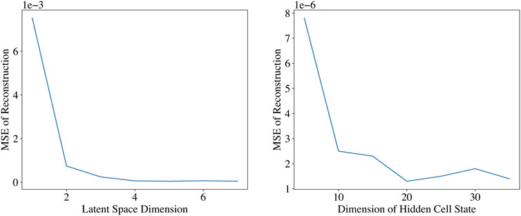
FIGURE 7. Left:Reconstruction error of the autoencoder with varying bottleneck layer dimensions during the ROM training, showing that the error plateaus after a 4D latent space. Right: Mean Squared Error of the Trained LSTM Network with Varying Cell State Dimension, showing that the error plateaus after a 20 dimensional cell state.

The architecture of the final autoencoder used is shown in Table 1. Both the encoder and decoder consist of 3-layer networks each with a single hidden layer. Non-linear tanh activation functions are used on all layers, with the exception of the layer prior to the bottleneck layer and the final output layer, where linear activations are used. Linear activations are generally used before outputs which are to be interpreted since a non-linear activation function limits the possible values to be output by the layer.

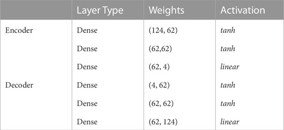
TABLE 1. Final architecture of the autoencoder used in the ROM.

5.2 LSTM training

The training of the LSTM network comprises the most challenging aspect of the ROM procedure, due to the large number of hyperparameters which must be tuned. To increase efficiency, a Nvidia Tesla P100 GPU was used for training, as provided through Google Colab hosted notebooks. The LSTM network considered consists of a single LSTM cell with a dense layer stacked on top of it. This network is trained to predict the response in the reduced space given the 4 input time series: the forces and moments in the x and y directions. As such the dense output layer has a fixed size of 4, since this layer corresponds to the dimensionality of the predicted output. Furthermore, the output layer is chosen to have a linear activation function per the standard for regression problems. This leaves the hidden state size of the LSTM cell as the key hyperparameter of the employed architecture, which dictates expressive power of the network. Generally, a higher hidden state size results in a more powerful network, albeit at a corollary increase in the number of parameters.

Further to the network architecture, some further important hyperparameters exist in the context of training, which severely affect performance. RNNs are trained using back propagation through time (BPTT)Goodfellow et al. (2016), similarly to standard back propagation, this involves a forward pass through the network to determine the error of prediction with the current parameters, followed by a backward pass in which the errors are propagated backwards through the network and the gradient of this error with respect to the parameters is found. Theoretically, we may pass the entire sequence to the network. Each training step then involves stepping through the entire time series of 600s in a forward pass, then propagating the error backwards through all time steps. Whilst the network may be trained by using the full length of the time series, this can become highly inefficient and memory intensive when considering long time histories Aicher et al. (2020). As such, it is common practice to make use of truncated BPTT. In truncated BPTT, each training step involves chunks of the total sequence of a given length. This increases efficiency in network training at the expense of having to choose the length of these chunks as another hyperparameter, which can significantly effect the rate of convergence Aicher et al. (2020).

In order to identify the optimal dimension of the hidden cell state, LSTM networks with varying cell state dimensions were trained and compared in terms of their predictive, one step ahead, performance on a validation set. The right hand subplot of Figure 7 plots the error of the different architectures of the LSTM network. A hidden cell state dimension of 20 was finally chosen, as the error decreased significantly up until a 20 dimensional state and then plateaued.

The final architecture used for the LSTM neural network is shown in Table 2. A single LSTM cell was used with a 20 dimensional hidden state vector and a tanh non-linear activation function. Stacked on the LSTM cell is a Dense layer with a 4 dimensional output and a linear activation function. In this case, 150 time steps were included for the BPTT algorithm Sutskever (2013), this corresponds to 3 s of response.

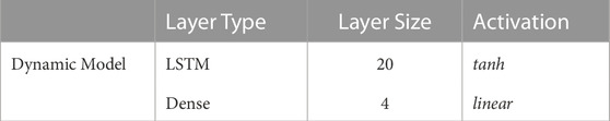
TABLE 2. Final architecture of the LSTM network used in the ROM.

6 ROM results

To test the accuracy of the trained ROM, the 69 input time series not used in the training stage are then fed as inputs to the ROM. The simulations are carried out using the ROM and compared to the results obtained from the FOM for the same input time series, using the normalised mean squared error (NMSE). This is the mean squared error normalised by the standard deviation of its DOF response. This is shown in Equation 3 wherein M is the number of DOFs and N the number of time steps, X the true response, $\widehat{X}$ the predicted response and σ meaning the standard deviation as defined in Equation 4. The NMSE as such, takes finds the mean squared error for each DOF individually and then normalises this mean squared error of each DOF by the standard deviation of the true response at this DOF. The NMSE is then the mean across all the DOFs of these normalised MSEs.

Figure 8 shows a violin plot of the NMSE values found for all 69 tested input time series with the wind speed represented by the color of each marker, from dark blue at 4 m/s to yellow at 28 m/s. The errors are distributed in two main lobes, with simulations in the first lobe comprising an extremely low NMSE error of less than 10^–4, while the second lobe is clustered between 2 − 4e-4. A single outlying simulation is caught with considerably larger NMSE error of 9.37 × 10⁻⁴. It is noteworthy that this highest error occurs from a simulation taken at the highest wind speed, which is outside of the range of speeds in the training set. Aside from this isolated outlier, no strong trend is noted between the wind speed and the error.

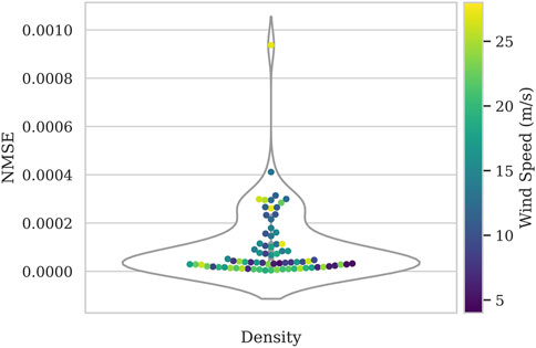
FIGURE 8. Violin plot how the NMSE error of the ROM simulations compared to the FOM is distributed, colored by wind speed from blue (lowest) to yellow (highest). The simulations exhibit very low NMSE values less than 4e − 4 with one outlying simulation with an error of 1e − 3.

In order to in practice understand what these NMSE values reveal in terms of discrepancy, the time series response of the FOM and ROM are further visually compared. Since it is unfeasible to visualise all DOFs of the system, few DOFs at the most critical locations on the monopile are monitored. The illustrated DOFs reflect the x, y, R_x and R_y response at the mud line, and at depths of 15m and 30 m. The upper subplot of Figure 9 shows such a visualisation for one of the tested time series with an NMSE of 1.56 × 10⁻⁴ hence locating it in the middle of the two main lobes of the violin plot. The ROM offers a good approximation of the reference FOM simulation in all of the monitored DOFs, once the steady state has been achieved. However, in the y displacement and R_x rotation, that the transient initial response is not perfectly captured by the ROM. The lack of fidelity in the transient regime is explainable in that the relevant dynamics in the transient response are significantly different to those in the stead-state regime. The transient dynamics usually contain much more in higher frequency ranges, however, since the majority of the data used for training the model is from the steady-state domain, the transient dynamics are less well approximated. If an application required that the transient response be better captured, this would be possible by increasing the amount of transient behaviour in the training data, or by weighting the cost function such that this data has more importance. Further, a more complex network may be required in order to capture both the transient and steady-state behaviour. In this use case, however, the lack of fidelity in the transient region is not considered a significant issue. This is because this initial transient response is anyway considered to be unrealistic, as it is a result of the immediate application of wind and wave loading from zero initial condition. Such a sudden loading example is not realistic during normal operation. The lower subplot of Figure 9 makes this more clear by displaying a zoomed view of the ROM prediction compared to the FOM prediction.

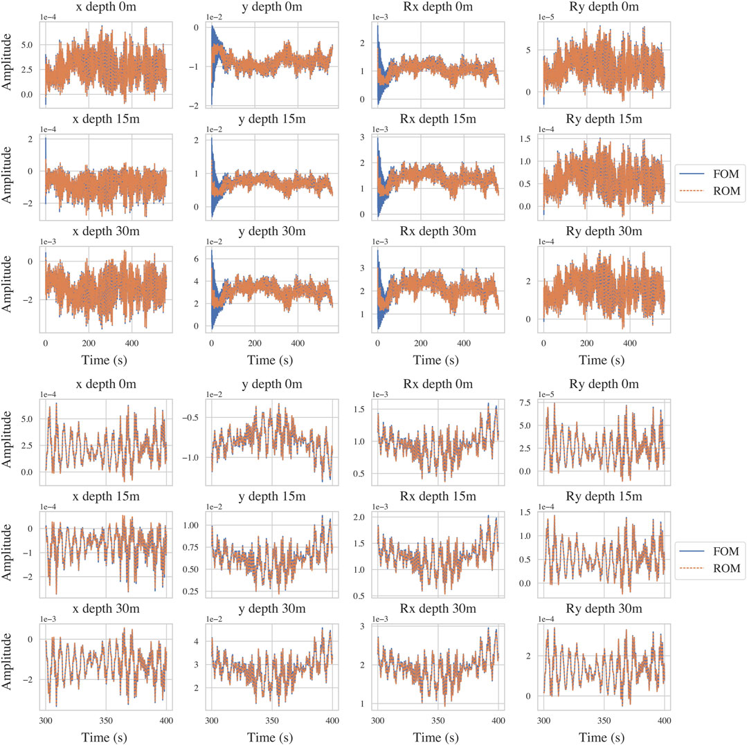
FIGURE 9. Upper: The time series response of the ROM (orange) compared against the reference FOM simulation (blue) for the x and y displacements in metres (1st and 2nd columns) and R_x and R_y rotations in rad (3rd and 4th columns) at depths of 0, 15 and 30 m (1st, 2nd and 3rd row) along the monopile. These results are taken from a simulation with NMSE of 1.56 × 10⁻⁴ carried out at a wind speed of 10 m/s and show excellent fidelity in the steady state response. Lower: A zoomed view of the upper plot highlighting the behaviour.

Figure 10 compares the frequency content of the response of the ROM and FOM predictions. The frequency content of the response is also captured with very high fidelity by the ROM.

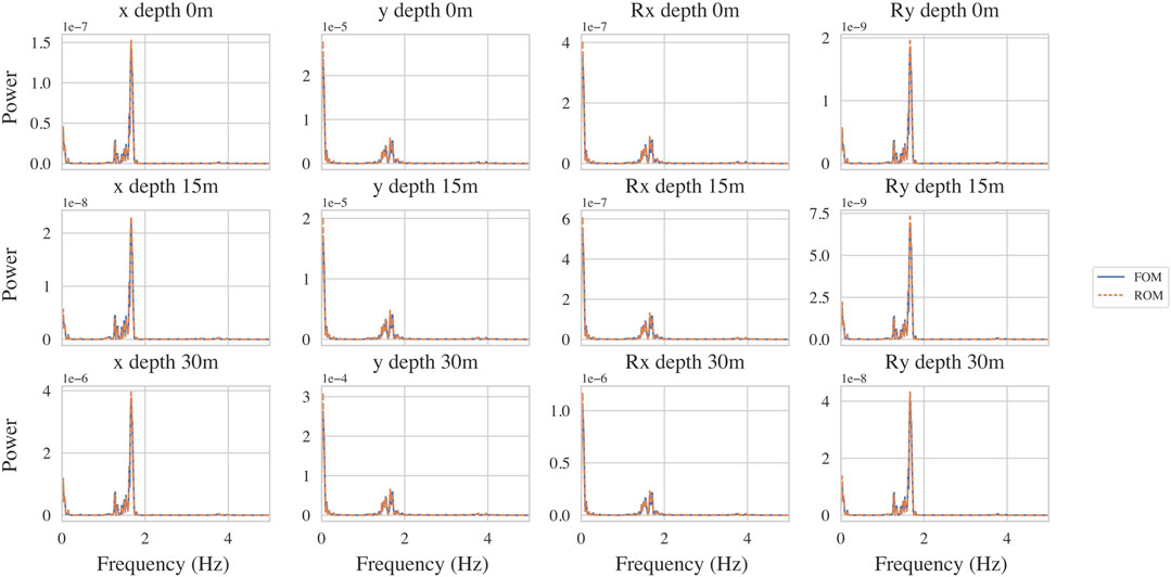
FIGURE 10. Comparison of frequency content of response of the ROM (orange) compared against the reference FOM simulation (blue) for the x and y displacements in m² (1st and 2nd columns) and R_x and R_y rotations in rad² (3rd and 4th columns) at depths of 0, 15 and 30 m (1st, 2nd and 3rd row) along the monopile. These results are taken from a simulation with NMSE of 1.56 × 10⁻⁴ carried out at a wind speed of 10 m/s and show excellent fidelity.

It is also worth illustrating the worst-case (outlier) performance of the model for the simulation which yielded a NMSE of 9.37 × 10⁻⁴, which corresponds to a wind speed of 28 m/s. The upper subplot of Figure 11 compares the time series response of the ROM and FOM for this worst performing simulation. The DOFs presented comprise of the x, y, R_x and R_y response at the mud line, at a depth of 15m, and at a depth of 30 m. For the x displacements and R_y rotations, the ROM performance is of good fidelity. However, in the y displacements and R_x rotations the ROM fails to adequately capture the reference behaviour, both missing certain peaks and displaying spurious peaks. This behaviour can be seen more closely in the lower subplot of Figure 11.

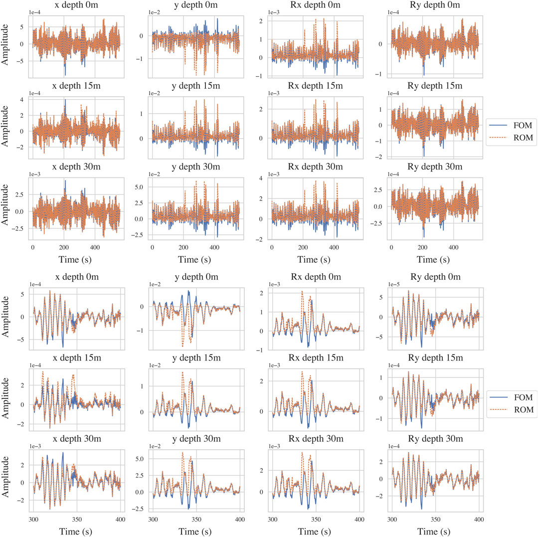
FIGURE 11. Upper: The time series response of the ROM (orange) compared against the reference FOM simulation (blue) for the x and y displacements in m (1st and 2nd columns) and R_x and R_y rotations in rad (3rd and 4th columns) at depths of 0, 15 and 30 m (1st, 2nd and 3rd row) along the monopile. These results are taken from the worst performing simulation with NMSE of 9.37 × 10⁻⁴ carried out at a wind speed of 28 m/s and show reasonable performance but with clear errors especially in the y displacements and R_x rotations. Lower: A zoomed view of the upper plot highlighting the behaviour.

Furthermore, from Figure 12 the spectrum of the ROM response is compared to the FOM response. It is clearly seen that the ROM inadequately captures the response of the y displacements and R_x rotations and suffers several spurious resonant peaks.

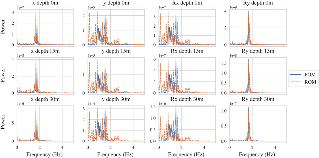
FIGURE 12. Comparison of the frequency content of the response of the ROM (orange) compared against the reference FOM simulation (blue) for the x and y displacements in m² (1st and 2nd columns) and R_x and R_y rotations in rad² (3rd and 4th columns) at depths of 0, 15 and 30 m (1st, 2nd and 3rd row) along the monopile. These results are taken from the worst performing simulation with NMSE of 9.37 × 10⁻⁴ carried out at a wind speed of 28 m/s and show reasonable performance but with clear spurious peaks in the spectra of the y displacements and R_x rotations.

In industrial settings, the full time series output by a simulation are often not used, rather certain features from them are taken and considered as the quantities of interest. Commonly used features are the maximum, minimum and standard deviation of the response. Figure 13 compares the maximum, minimum and standard deviation of the response in the x, y, R_x and R_y DOFs at the uppermost node of the monopile at a depth of 0 m as predicted by the FOM and ROM. The ROM can be seen to also very accurately recreate these values of interest across all 75 simulations. Notably, even the failed simulation observed in the full time series is not shown to have a great impact on the fidelity with respect to these quantities of interest.

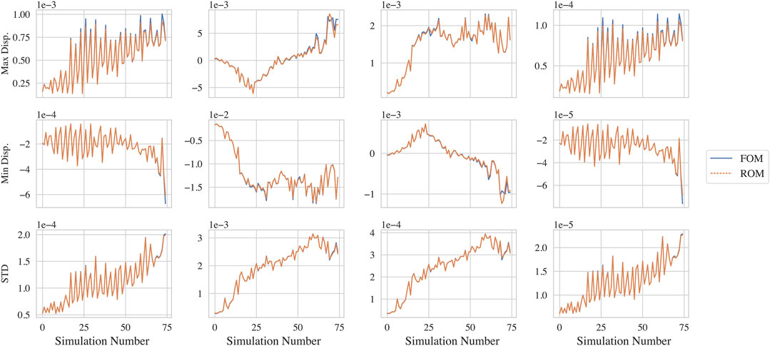
FIGURE 13. Comparison of the maximum (1st row), minimum (2nd row) and standard deviation (3rd row) of the displacement values during all 75 simulations as output by the ROM (orange) and FOM (blue). These measurements are for the x and y displacements in m2 (1st and 2nd columns) and R_x and R_y rotations in rad (3rd and 4th columns) at a depth of 0 m on the monopile.

An important aspect of any ROM lies in reduction in the computational time required against the FOM. In this case, a comparison was made between the prediction time of the ROM and Abaqus simulations on the same computing hardware, Intel^® Core™ i7-6700 CPU, 3.40 GHz 8 core Processor. In both cases a 600 s simulation was carried out. As Table 3 reports, the ROM provides a large benefit in terms of computational savings, delivering over 300 times of speed up. The ROM further allows for the simulation to be carried out significantly faster than real time, contrary to the FOM which is approximately four times slower than real time.

TABLE 3. Computational time of the ROM vs Abaqus for 600 s of simulation.

6.1 Recognising a failed simulation

Since the proposed framework describes a data-driven approach, it is expected that outliers will occur, particularly in an extrapolation setting. It is important that such outliers be detectable without having to run FOM simulations for comparison as this somewhat defeats the purpose of creating a ROM. With regards to the simulations carried out in this work, a single simulation is considered to have failed, comprising an error of roughly 10 times the mean error. Having observed the spectra of the response of this simulation in Figure 12, spurious peaks could be observed which do not appear in the FOM simulations. To try to identify this failed simulation, we can look at the spectra of all ROM simulations carried out in an attempt to check for anomalies. Importantly, the FOM simulations are not required in this error check.

In Figure 14, the spectra of the response for all 75 ROM simulations at the 92nd DOF (corresponding to the y displacement at the top of the monopile) is plotted. This figure shows that the spurious peaks in the spectra can be identified when com, paring against the further ROM simulations. The 74th simulation, which is indeed the simulation which failed, can easily be identified as differing from the remaining simulations. It can clearly be seen that the 74th simulation exhibits several peaks around 0.25–0.75 Hz unlike the remaining simulations. These spurious peaks further form a main difference between the spectra of the failed simulation when compared against the equivalent FOM simulation. These peaks can thus serve as a means to identifying failed ROM simulations.

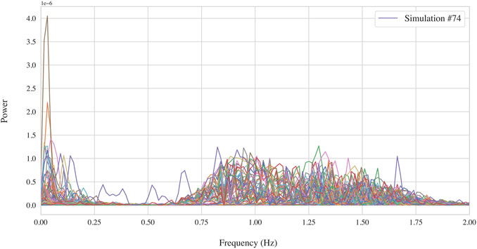
FIGURE 14. Spectral response of all 75 of the ROM simulations a the 92nd DOF, corresponding to the R_x rotation at a depth of 0 m. The 74th simulation may be seen to be an outlier exhibiting spurious peaks between 0.25 and 0.75 Hz.

To demonstrate how detecting such a failed simulation may be carried out practically, we demonstrate one such method. Firstly, from examining the Spectra as shown in Figure 14 we identify that the frequency range between 0.25 and 0.75 Hz seems to demonstrate some anomalous behaviour and so we focus our analysis on this area. We wish to do anomaly detection using this region of the spectra as such we take as features, the amplitude of the spectra at each of the frequency bins between 0.25 and 0.75 Hz, this corresponds to 40 amplitude values. This gives us 40 dimensional features for each of the 75 simulation runs, such high dimensional features are cumbersome and probably redundant, as such, a PCA reduction is applied to these features and the dimensionality reduced to 2. These features are visualised in Figure 15 in which the 2 principal components are plotted against one another for each of the 75 simulations. In this plot there is again one obvious outlier which is indeed the 74th simulation which we had previously identified as failing. To fully formalise this novelty detection methodology, we would then introduce a distance metric such as the Mahalanobis squared distance Mahalanobis (1936), then a training dataset would be created for which the simulations are known to be good, outliers would then be detectable based on their Mahalanobis distance from the centroid of such a training set. A similar process is shown in much more detail by Worden et al. Worden et al. (2000).

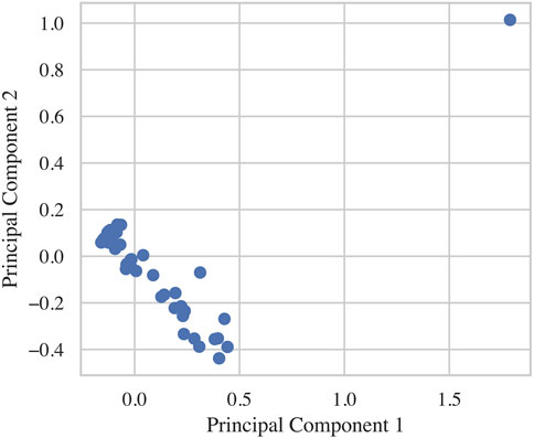
FIGURE 15. Plot of the first 2 principal components extracted from the spectral amplitudes between 0.25 and 0.75 Hz for all the 75 ROM simulations. One simulation represents a clear outlier, which corresponds to the simulation judged to have failed based on NMSE against the FOM.

7 Conclusion

This work demonstrates application of a recently developed non-linear ROM methodology, the AE-LSTM ROM, for treating the SSI problem in offshore wind turbine structures. The method reflects a data-driven approach requiring no assumptions on the type of non-linearity present and can be flexibly applied across a broad range of non-linear dynamical systems. The method is trained, using data extracted from FE simulations on the non-linear SSI problem of an offshore wind turbine monopile.

The following conclusions are drawn.

• The AE-LSTM methodology can capture the behaviour of the modelled non-linear SSI problem, with training conducted on only 6 time series, and accurately recreate the response for unseen input forcings.

• The ROM was successful in very significantly reducing the simulation time required when compared to the FOM, reducing the computational time by a factor of over 300 times.

• A single simulation was considered to have failed, yielding significantly higher error than the others. However, it is shown that an error metric can be adopted to identify such a failure without requiring the FOM response as comparison.

A limitation of the method is that the input dimensionality is currently not reduced at all. This is not an issue in the presented example where the forcing occurs only at the boundary, however, were the input high dimensional, e.g., for a distributed load, then this would likely scale badly and require dimensionality reduction of the input. One method to rectify this could be to add an additional layer to the network between the inputs and the LSTM layer. Such a layer would then reduce the dimension of the input data before passing it to the LSTM cell. Further development with regards to the ROM of the SSI problem would involve coupling it to the existing aeroelastic simulation of the wind turbine above the mudline. To achieve this, it would be necessary to additionally generate tangent structural matrices for each time step of the ROM in order to successfully couple the ROM to the existing simulation framework Arramounet et al. (2019).

Data availability statement

The datasets presented in this study can be found in online repositories. The names of the repository/repositories and accession number(s) can be found below: https://github.com/tomsimpson74/AE-LSTM_ROM.

Author contributions

TS: Methodology, carrying out FOM simulations, training the ROM and manuscript preparation. ND: Methodology, Review and editing. PC: Problem definition, Verifying and desiging the FOM, Review and editing. NM: Problem definition, Design and specification of the FOM and loading conditions, Review and editing. EC: Methodology Review and editing and Funding acquisition.

Funding

This project has received funding from the European Union’s Horizon 2020 research and innovation programme under the Marie Skłodowska-Curie grant agreement No 764547 and from the EPSRC under grant agreement EP/R004900/1.

Conflict of interest

The authors declare that the research was conducted in the absence of any commercial or financial relationships that could be construed as a potential conflict of interest.

Publisher’s note

All claims expressed in this article are solely those of the authors and do not necessarily represent those of their affiliated organizations, or those of the publisher, the editors and the reviewers. Any product that may be evaluated in this article, or claim that may be made by its manufacturer, is not guaranteed or endorsed by the publisher.

Supplementary material

The Supplementary Material for this article can be found online at: https://www.frontiersin.org/articles/10.3389/fenrg.2023.1128201/full#supplementary-material

References

Abdullahi, A., Wang, Y., and Bhattacharya, S. (2020). Comparative modal analysis of monopile and jacket supported offshore wind turbines including soil-structure interaction. Int. J. Struct. Stab. Dyn. 20, 2042016. doi:10.1142/s021945542042016x
Abhinav, K., and Saha, N. (2018). Nonlinear dynamical behaviour of jacket supported offshore wind turbines in loose sand. Mar. Struct. 57, 133–151. doi:10.1016/j.marstruc.2017.10.002
Adhikari, S., and Bhattacharya, S. (2011). Vibrations of wind-turbines considering soil-structure interaction. Wind Struct. 14, 85–112. doi:10.12989/was.2011.14.2.085
Aicher, C., Foti, N. J., and Fox, E. B. (2020). “Adaptively truncating backpropagation through time to control gradient bias,” in Proceedings of The 35th Uncertainty in Artificial Intelligence Conference, Israel, 1-17, 2020.
Amsallem, D., and Farhat, C. (2008). Interpolation method for adapting reduced-order models and application to aeroelasticity. AIAA J. 46, 1803–1813. doi:10.2514/1.35374
Arramounet, V., de Winter, C., Maljaars, N., Girardin, S., and Robic, H. (2019). “Development of coupling module between BHawC aeroelastic software and OrcaFlex for coupled dynamic analysis of floating wind turbines,” in Jornal of Physics: Conference Series, Norway, 16–18 January 2019.
Baldi, P., and Hornik, K. (1989). Neural networks and principal component analysis: Learning from examples without local minima. Neural Netw. 2, 53–58. doi:10.1016/0893-6080(89)90014-2
Bayer, J. S. (2015). Learning sequence representations. Ph.D. Thesis. München, Germany: Technische Universität München.
Cao, G., Chen, Z., Wang, C., and Ding, X. (2020). Dynamic responses of offshore wind turbine considering soil nonlinearity and wind-wave load combinations. Ocean. Eng. 217, 108155. doi:10.1016/j.oceaneng.2020.108155
Carlberg, K., and Farhat, C. (2008). “A compact proper orthogonal decomposition basis for optimization-oriented reduced-order models,” in 12th AIAA/ISSMO Multidisciplinary Analysis and Optimization Conference, Canada, 12 September 2008.
Cenedese, M., Axås, J., Bäuerlein, B., Avila, K., and Haller, G. (2022). Data-driven modeling and prediction of non-linearizable dynamics via spectral submanifolds. Nat. Commun. 13, 872. doi:10.1038/s41467-022-28518-y
Champneys, M., Tsialiamanis, G., Rogers, T., Dervilis, N., and Worden, K. (2022). On the dynamic properties of statistically-independent nonlinear normal modes. Mech. Syst. Signal Process. 181, 109510. doi:10.1016/j.ymssp.2022.109510
Chen, S., and Billings, S. A. (1989). Modelling and analysis of non-linear time series. Int. J. Control 50, 2151–2171. doi:10.1080/00207178908953491
Chinesta, F., Ladeveze, P., and Cueto, E. (2011). A short review on model order reduction based on proper generalized decomposition. Archives Comput. Methods Eng. 18, 395–404. doi:10.1007/s11831-011-9064-7
Craig, R., and Bampton, M. (1968). Coupling of substructures for dynamic analyses. AIAA J. 6, 1313–1319. doi:10.2514/3.4741
Craig, R., and Kurdila, A. (2006). Fundamentals of structural dynamics. Hoboken, New Jersey, USA: John Wiley and Sons.
Dervilis, N., Simpson, T., Wagg, D., and Worden, K. (2019). Nonlinear modal analysis via non-parametric machine learning tools. Strain 55, e12297. doi:10.1111/str.12297
Devriendt, C., Magalhães, F., Weijtjens, W., Sitter, G. D., Cunha, Á., and Guillaume, P. (2014). Structural health monitoring of offshore wind turbines using automated operational modal analysis. Struct. Health Monit. 13, 644–659. doi:10.1177/1475921714556568
Dnv, D. (2014). “Offshore standard: Design of offshore wind turbine structures,”. Tech. Rep. DNV-OS-J101, DNV AS, Høvik, Norway.
Farhat, C., Avery, P., Chapman, T., and Cortial, J. (2014). Dimensional reduction of nonlinear finite element dynamic models with finite rotations and energy-based mesh sampling and weighting for computational efficiency. Int. J. Numer. Methods Eng. 98, 625–662. doi:10.1002/nme.4668
Graves, A., Fernández, S., Liwicki, M., Bunke, H., and Schmidhuber, J. (2007). “Unconstrained online handwriting recognition with recurrent neural networks,” in Proceedings of the 20th International Conference on Neural Information Processing Systems, Korea, November 3-7, 2013.
Harte, M., Basu, B., and Nielsen, S. (2012). Dynamic analysis of wind turbines including soil-structure interaction. Eng. Struct. 45, 509–518. doi:10.1016/j.engstruct.2012.06.041
Hasselmann, K., Barnett, T. P., Bouws, E., Carlson, H., Cartwright, D. E., Enke, K., et al. (1973). Measurements of wind-wave growth and swell decay during the joint north sea wave project (jonswap). Ergaenzungsh. zur Dtsch. Hydrogr. Z. Reihe A.
Hinton, G. E., and Salakhutdinov, R. R. (2006). Reducing the dimensionality of data with neural networks. Science 313, 504–507. doi:10.1126/science.1127647
Hochreiter, S., and Schmidhuber, J. (1997). Long short-term memory. Neural Comput. 9, 1735–1780. doi:10.1162/neco.1997.9.8.1735
Holden, D., Saito, J., Komura, T., and Joyce, T. (2015). “Learning motion manifolds with convolutional autoencoders,” in SIGGRAPH Asia 2015 Technical Briefs, Kobe Japan, November 2 - 6, 2015.
Hu, W.-H., Thöns, S., Rohrmann, R. G., Said, S., and Rücker, W. (2015b). Vibration-based structural health monitoring of a wind turbine system part ii: Environmental/operational effects on dynamic properties. Eng. Struct. 89, 273–290. doi:10.1016/j.engstruct.2014.12.035
Hu, W.-H., Thöns, S., Rohrmann, R. G., Said, S., and Rücker, W. (2015a). Vibration-based structural health monitoring of a wind turbine system. part i: Resonance phenomenon. Eng. Struct. 89, 260–272. doi:10.1016/j.engstruct.2014.12.034
Izenman, A. J. (2012). Introduction to manifold learning. WIREs Comput. Stat. 4, 439–446. doi:10.1002/wics.1222
Jain, S., Tiso, P., Rutzmoser, J. B., and Rixen, D. J. (2017). A quadratic manifold for model order reduction of nonlinear structural dynamics. Comput. Struct. 188, 80–94. doi:10.1016/j.compstruc.2017.04.005
Jardine, R. J., Potts, D. M., Fourie, A. B., and Burland, J. B. (1986). Studies of the influence of non-linear stress–strain characteristics in soil–structure interaction. Géotechnique 36, 377–396. doi:10.1680/geot.1986.36.3.377
Kerschen, G., Jean-claude, G., Vakakis, A. F., and Bergman, L. A. (2005). The method of proper orthogonal decomposition for dynamical characterization and order reduction of mechanical systems: An overview. Nonlinear Dyn. 41, 147–169. doi:10.1007/s11071-005-2803-2
Kerschen, G., Peeters, M., Golinval, J., and Vakakis, A. (2009). Nonlinear normal modes, part i: A useful framework for the structural dynamicist. Mech. Syst. Signal Process. 23, 170–194. doi:10.1016/j.ymssp.2008.04.002
Kingma, D. P., and Ba, J. (2015). “Adam: A method for stochastic optimization,” in 3rd International Conference on Learning Representations, ICLR 2015 - Conference Track Proceedings, USA, May 7-9, 2015.
Kingma, D. P., and Welling, M. (2014). “Auto-encoding variational bayes,” in 2nd International Conference on Learning Representations, ICLR 2014 - Conference Track Proceedings, Canada, April 14-16, 2014.
Lee, K., and Carlberg, K. T. (2020). Model reduction of dynamical systems on nonlinear manifolds using deep convolutional autoencoders. J. Comput. Phys. 404, 108973. doi:10.1016/j.jcp.2019.108973
Lopez, R., and Atzberger, P. J. (2020). Variational autoencoders for learning nonlinear dynamics of physical systems. USA: CSAI.
Mahalanobis, P. C. (1936). On the generalized distance in statistics. Calcutta: National Institute of Science of India.
Martakis, P., Taeseri, D., Chatzi, E., and Laue, J. (2017). A centrifuge-based experimental verification of soil-structure interaction effects. Soil Dyn. Earthq. Eng. 103, 1–14. doi:10.1016/j.soildyn.2017.09.005
Martinez-Luengo, M., Kolios, A., and Wang, L. (2016). Structural health monitoring of offshore wind turbines: A review through the statistical pattern recognition paradigm. Renew. Sustain. Energy Rev. 64, 91–105. doi:10.1016/j.rser.2016.05.085
Matlock, H. (1970). “Correlation for design of laterally loaded piles in soft clay,” in OTC Offshore Technology Conference, Houston, April 1970.
Matlock, H., and Reese, L. C. (1960). Generalized solutions for laterally loaded piles. J. Soil Mech. Found. Div. 86, 63–92. doi:10.1061/JSFEAQ.0000303
Mylonakis, G., and Gazetas, G. (2000). Seismic soil-structure interaction: Beneficial or detreimental? J. Earthq. Eng. 4, 277–301. doi:10.1080/13632460009350372
Pando, M., Ealy, C., Filz, G., Lesko, J., and Hoppe, E. (2006). A laboratory and field study of composite piles for bridge substructures. Tech. Rep. FHWA-HRT-04-043. United States: Federal Highway Administration.
Pimenta, F., Pacheco, J., Branco, C. M., Teixeira, C. M., and Magalhães, F. (2020). Development of a digital twin of an onshore wind turbine using monitoring data. J. Phys. Conf. Ser. 1618, 022065. doi:10.1088/1742-6596/1618/2/022065
Poncelet, F., Kerschen, G., Golinval, J.-C., and Verhelst, D. (2007). Output-only modal analysis using blind source separation techniques. Mech. Syst. Signal Process. 21, 2335–2358. doi:10.1016/j.ymssp.2006.12.005
Rogers, T. J., Schön, T. B., Lindholm, A., Worden, K., and Cross, E. J. (2019). Identification of a duffing oscillator using particle gibbs with ancestor sampling. J. Phys. Conf. Ser. 1264, 012051. doi:10.1088/1742-6596/1264/1/012051
Rumelhart, D. E., and McClelland, J. L. (1987). Learning internal represetnations by error propagation. USA: MIT Press.
Sadorksy, P. (2021). Wind energy for sustainable development: Driving factors and future outlook. J. Clean. Prod. 289, 125779. doi:10.1016/j.jclepro.2020.125779
Sajeer, M. M., Mitra, A., and Chakraborty, A. (2021). Multi-body dynamic analysis of offshore wind turbine considering soil-structure interaction for fatigue design of monopile. Soil Dyn. Earthq. Eng. 144, 106674. doi:10.1016/j.soildyn.2021.106674
Sakurada, M., and Yairi, T. (2014). “Anomaly detection using autoencoders with nonlinear dimensionality reduction,” in Proceedings of the MLSDA 2014 2nd Workshop on Machine Learning for Sensory Data Analysise, New York, 2 December 2014.
Simpson, T., Dervilis, N., and Chatzi, E. (2021). Machine learning approach to model order reduction of nonlinear systems via autoencoder and lstm networks. J. Eng. Mech. 147, 04021061. doi:10.1061/(ASCE)EM.1943-7889.0001971
Simpson, T., Tsialiamanis, G., Dervilis, N., Worden, K., and Chatzi, E. (2023). “On the use of variational autoencoders for nonlinear modal analysiss,” in Nonlinear structures and systems (Orlando, Florida: Springer International Publishing).
Solman, H., Kirkegaard, J. K., Smits, M., Van Vliet, B., and Bush, S. (2022). Digital twinning as an act of governance in the wind energy sector. Environ. Sci. Policy 127, 272–279. doi:10.1016/j.envsci.2021.10.027
Sudret, B., Marelii, S., and Wiart, J. (2017). “Surrogate models for uncertainty quantification: An overview,” in 2017 11th European Conference on Antennas and Propagation, France, 19-24 March 2017.
Sutskever, I. (2013). Training recurrent neural networks. Toronto, Canada: Ph.D. thesis, University of Toronto.
Tatsis, K., Dertimanis, V., Abdallah, I., and Chatzi, E. (2017). A substructure approach for fatigue assessment on wind turbine support structures using output-only measurements. Procedia Eng. 199, 1044–1049. International Conference on Structural Dynamics, EURODYN 2017. doi:10.1016/j.proeng.2017.09.285
Tatsis, K., Wu, L., Tiso, P., and Chatzi, E. (2018). State estimation of geometrically non-linear systems using reduced-order models. Europe: Taylor and Francis.
Tsialiamanis, G., Champneys, M., Dervilis, N., Wagg, D., and Worden, K. (2022). On the application of generative adversarial networks for nonlinear modal analysis. Mech. Syst. Signal Process. 166, 108473. doi:10.1016/j.ymssp.2021.108473
University of Michigan (2021). Wind energy fact sheet. Tech. Rep. Pub. No. CSS07-09. Michigan: University of Michigan.
Vincent, P., Larochelle, H., Bengio, Y., and Manzagol, P.-A. (2008). “Extracting and composing robust features with denoising autoencoders,” in Proceedings of the 25th International Conference on Machine Learning, Helsinki Finland, July 5 - 9, 2008.
Vlachas, K., Tatsis, K., Agathos, K., Brink, A. R., and Chatzi, E. (2021). A local basis approximation approach for nonlinear parametric model order reduction. J. Sound Vib. 502, 116055. doi:10.1016/j.jsv.2021.116055
Vlachas, K., Tatsis, K., Agathos, K., Brink, A. R., Quinn, D., and Chatzi, E. (2022a). “Parametric model order reduction for localized nonlinear feature inclusion,” in Advances in nonlinear dynamics. Editors W. Lacarbonara, B. Balachandran, M. J. Leamy, J. Ma, J. A. Tenreiro Machado, and G. Stepan (Cham: Springer International Publishing).
Vlachas, P. R., Arampatzis, G., Uhler, C., and Koumoutsakos, P. (2022b). Multiscale simulations of complex systems by learning their effective dynamics. Nat. Mach. Intell. 4, 359–366. doi:10.1038/s42256-022-00464-w
Vlachas, P. R., Byeon, W., Wan, Z. Y., Sapsis, T. P., and Koumoutsakos, P. (2018). Data-driven forecasting of high-dimensional chaotic systems with long short-term memory networks. Proc. R. Soc. A 474, 20170844. doi:10.1098/rspa.2017.0844
Wagg, D., Worden, K., Barthorpe, R., and Gardner, P. (2020). Digital twins: State-of-the-Art and future directions for modeling and simulation in engineering dynamics applications. ASCE-ASME J Risk Uncert Engrg Sys Part B Mech Engrg 6. doi:10.1115/1.4046739
Wang, H., and Wu, T. (2020). Knowledge-enhanced deep learning for wind-induced nonlinear structural dynamic analysis. J. Struct. Eng. 146. doi:10.1061/(asce)st.1943-541x.0002802
Whyte, S., Burd, H., Martin, C., and Rattley, M. (2020). Formulation and implementation of a practical multi-surface soil plasticity model. Comput. Geotechnics 117, 103092. doi:10.1016/j.compgeo.2019.05.007
Wold, S., Esbensen, K., and Geladi, P. (1987). Principal component analysis. Chemom. Intelligent Laboratory Syst. 2, 37–52. doi:10.1016/0169-7439(87)80084-9
Wolf, T., Rasmussen, K., Hansen, M., Roesen, H., and Ibsen, L. (2013). “Assessment of p-y curves from numerical methods for a non-slender monopile in cohesionless soil,” in DCE technical memorandum (Denmark: Department of Civil Engineering, Aalborg University).
Wong, H. L. (1975). Dynamic soil-structure interaction. Ph.D. Thesis. Pasadena, California, USA: California Institute of Technology.
Worden, K., and Green, P. L. (2016). A machine learning approach to nonlinear modal analysis. Mech. Syst. Signal Process. 84, 34–53. doi:10.1016/j.ymssp.2016.04.029
Worden, K., Manson, G., and Fieller, N. (2000). Damage detection using outlier analysis. J. Sound Vib. 229, 647–667. doi:10.1006/jsvi.1999.2514
Wu, L., and Tiso, P. (2016). Nonlinear model order reduction for flexible multibody dynamics: A modal derivatives approach. Multibody Syst. Dyn. 36, 405–425. doi:10.1007/s11044-015-9476-5
Wu, Y., Schuster, M., Chen, Z., Le, Q. V., Norouzi, M., Macherey, W., et al. (2016). “Google’s neural machine translation system: Bridging the gap between human and machine translation,”. CoRR.
Yoo, Y., Yun, S., Chang, H. J., Demiris, Y., and Choi, J. Y. (2017). “Variational autoencoded regression: High dimensional regression of visual data on complex manifold,” in 2017 IEEE Conference on Computer Vision and Pattern Recognition, USA, July 26 2017.
Zhang, R., Liu, Y., and Sun, H. (2020). Physics-informed multi-lstm networks for metamodeling of nonlinear structures. Comput. Methods Appl. Mech. Eng. 369, 113226. doi:10.1016/j.cma.2020.113226
Keywords: SSI, rom, LSTM, autoencoder (AE), non-linear, machine learning
Citation: Simpson T, Dervilis N, Couturier P, Maljaars N and Chatzi E (2023) Reduced order modeling of non-linear monopile dynamics via an AE-LSTM scheme. Front. Energy Res. 11:1128201. doi: 10.3389/fenrg.2023.1128201
Received: 20 December 2022; Accepted: 20 February 2023;
Published: 06 March 2023.
Edited by:
Shan Wang, University of Lisbon, PortugalReviewed by:
Xiaoxian Guo, Shanghai Jiao Tong University, ChinaArash Abbasnia, University of Lisbon, Portugal
Copyright © 2023 Simpson, Dervilis, Couturier, Maljaars and Chatzi. This is an open-access article distributed under the terms of the Creative Commons Attribution License (CC BY). The use, distribution or reproduction in other forums is permitted, provided the original author(s) and the copyright owner(s) are credited and that the original publication in this journal is cited, in accordance with accepted academic practice. No use, distribution or reproduction is permitted which does not comply with these terms.
*Correspondence: Thomas Simpson, simpson@ibk.baug.ethz.ch