Short-Term Forecasting and Uncertainty Analysis of Photovoltaic Power Based on the FCM-WOA-BILSTM Model

1 Introduction

In recent years, the demand for energy has been growing under the rapid economic development. Solar energy is the main clean energy source, and with gradual maturity of photovoltaic power generation technology and the increasing need to improve the global energy structure (Fei et al., 2016; Jin et al., 2021), photovoltaic power generation has been able to develop rapidly. However, photovoltaic power has strong randomness and volatility, and it is easy to cause a volatile impact on the power grid when photovoltaic power is connected to the grid, affecting the stable and safe operation of the power system (Guang et al., 2021), which brings certain difficulties to the dispatch of the power system, so the accuracy of photovoltaic power generation power prediction is of great research significance.

When the inner resolution of photovoltaic power generation is 15 min, it can be divided into ultra-short-term prediction (15 min–4 h), short-term prediction (4 h–3 days), and medium and long-term prediction (in months and years). The short-term photovoltaic probability is the research object of this paper. The existing PPF is mainly divided into direct method and indirect method (Changwei et al., 2019), of which the indirect method is mainly combined with the physical power generation principle of photovoltaic power plants (Ma et al., 2014; Almonacid et al., 2014). By establishing a physical model to predict the solar irradiance received by the ground or the solar irradiance received on the surface of the photovoltaic panels, and then predict the photovoltaic power generation power according to the various parameters of the photovoltaic power station and the solar irradiation intensity (Jiang et al., 2021). However, due to the complexity of physical modeling, the numerical weather forecasting update frequency is low, so the prediction effect of physical methods in ultra-short-term forecasting is often not ideal, and it is only suitable for medium-term, long-term, and short-term forecasting. The direct method relies on historical data to directly predict the photovoltaic power generation power, the modeling is relatively simple, and the forecast cost is relatively low, so it is widely used in the short-term prediction of photovoltaic power. For a long time, domestic and foreign scholars have done a lot of research on the short-term prediction of optical volt power in the direct method to solve the problems of photovoltaic grid connection to maintain the stability of the power system. Researchers have successively proposed support vector machine (SVM) (Mayer and Gróf, 2021), Markov chain (Hu and Zhang, 2018), limit learning machine (Wang, 2018), artificial neural network (ANN) (López Gómez et al., 2020), time series prediction and other methods (Zhu et al., 2019; Singh et al., 2021). Traditional ANN achieves power prediction by establishing a mapping between input data and output data, and the lack of consideration of time correlation in the data series makes it impossible for neural network models to capture the relationship between data and time, which limits its application in time series forecasting methods. Afterward, with the development of artificial intelligence (AI), the deep learning algorithm model represented by a recurrent neural network (RNN) (Li et al., 2019) has been widely used in the field of short-term PV power prediction. RNN is mainly used to process time-series data, but it is prone to long-term dependence. Long short-term memory (LSTM) introduces a gate structure on the basis of RNN structure, realizes the selective storage function of historical information, and solves the long-term dependency problem of RNN. LSTM is widely used in the fields of stock price forecasting, biomedicine, and power forecasting. Wu et al. (2022) have developed a cancer risk prediction tool for cancer through LSTM models, which works best with irregular data by comparing them with other ML models. These risk prediction tools are useful to direct subjects to further screening sooner, resulting in earlier detection of occult tumors. The water demand point forecasting will encounter uninformative and unreliable problems when the uncertainty level of data increases. A hybrid model (KDE-PSO-LSTM), which combines long-short-term memory networks (LSTM) with kernel density estimation (KDE) optimized by using the particle swarm optimization (PSO) algorithm, is proposed by Du et al. (2022) to acquire the water demand prediction interval (PI) to quantify the likely uncertainties in the predictions. Experimental results show that the proposed KDE-PSO-LSTM model generates better comprehensive performance than other models. Therefore, it can be demonstrated that the KDE-PSO-LSTM model can provide reliable decision support to policy-makers for making the optimal water supply management decision. Wang et al. (2020) proposed a photovoltaic ultra-short-term power output prediction method based on long short-term memory (LSTM). This method can not only mine the spatial and temporal correlation between the output and related input variables but has also been greatly developed in the field of complex time series prediction. This method has good prediction accuracy for the prediction of large data time series, but the determination of model parameters is troublesome. If it is directly applied to other practical prediction problems, the effect may not be very ideal. A single predictive model tends to have lower prediction accuracy, with the rapid development of deep learning, the accuracy of combined predictive models has been significantly improved compared with single predictive models. In addition, LSTM has too many internal parameters, and the model training time is long, which is prone to overfitting. Liu and Liu (2021) used genetic algorithms (GA) to optimize LSTM models to improve wind power forecasting. By analyzing the model prediction results of LSTM-CNN and GA-LSTM-CNN and comparing them with the actual power, the results show that the GA-LSTM-CNN prediction model has high accuracy. Tuerxun et al. (2022) proposed to build an optimized LSTM based on the modified condor search (MBES) algorithm to construct an MBES-LSTM model for short-term power prediction, thereby solving the problem that the choice of LSTM hyperparameters may affect the prediction results. The experimental results show that compared with the PSO-RBF, PSO-SVM, LSTM, PSO-LSTM, and BES-LSTM prediction models, the MBES-LSTM model can effectively improve the accuracy of wind farm prediction. Liu et al. (2021) proposed the dragonfly algorithm to optimize the short-term probability prediction of LSTM neural network. The dragonfly algorithm is used to optimize the super parameters of LSTM neural network, and the LSTM neural network prediction model is established according to the obtained optimal parameters. Finally, the DA-LSTM prediction model constructed using the optimum hyperparameters obtains the prediction results. The simulation results of the study show that compared with the traditional prediction model and the LSTM model, the DA-LSTM model can effectively make short-term predictions of wind power and has higher prediction accuracy. These authors mainly use some traditional optimization algorithms to optimize the parameter values of LSTM, thereby improving the prediction accuracy of LSTM. Due to the large number of internal parameters of LSTM, the long training time of the model, and the tendency to overfit, the effect of traditional optimization algorithms is not very ideal. With the development of science and technology, the whale optimization algorithm (WOA) (Gharehchopogh and Gholizadeh, 2019) has been introduced, which has the advantages of simple structure, fast convergence speed, and high convergence accuracy, and has been widely used in parameter optimization. Shang et al. (2020) proposed the use of least squares support vector machine (SVM), limit learning machine (ELM), and generalized regression neural network for power load prediction. In addition, the model uses a heuristic algorithm, the whale optimization algorithm (WOA), to optimize the weight coefficients. The proposed model was applied to electricity price forecasting and compared with the benchmark method. Experimental results show that the model can not only obtain accurate results for short-term power load prediction but also has good accuracy for electricity price prediction in the same period. However, we have rarely seen studies of optimizing other algorithms with WOA, especially the study of optimizing LSTM models with WOA. At the same time, the above prediction method only considers the one-way data information flow, ignores the impact of the transformation law of the reverse data sequence on the short-term prediction, and insufficient consideration is given to the time correlation and periodicity of the data. When the input time series is long, the sequence information is easily lost, and the prediction accuracy of the model is not high. Xie et al. (2020) used wavelet decomposition to extract the time domain information and frequency domain information of the input time series. Then, considering the bidirectional information flow, a bi-directional long-short-term memory network (BILSTM) is used for prediction, and an attention mechanism is introduced to give different weights to the hidden states of BILSTM by mapping the weighting and learning parameter matrix so as to selectively obtain more effective information. Finally, the simulation verification is carried out using the actual data. Simulation results show that the proposed BILSTM model has good predictive performance compared with the LSTM model. These authors mainly use some optimization algorithms to optimize the parameter values of neural network model models, thereby improving the prediction accuracy of the model. They did not consider the impact of weather clustering on prediction accuracy nor analyze the uncertainty of forecasting power.

Accurate analysis of PPF uncertainty is important for supporting the dispatching of the power grid and reducing the rotating reserve capacity of power generation equipment (Liu et al., 2018). The uncertainty analysis of PPF is mainly quantified by the confidence interval, which is usually described by the parametric estimation method and the non-parametric estimation method (Lv et al., 2021). The parameter estimation method needs to assume in advance that the photovoltaic power prediction error is a fixed empirical value or assume that the error distribution is a specific distribution form (Liu et al., 2018), beta (Von Loeper et al., 2020), gamma (Sun et al., 2020), Laplace mixture distribution (Elmagbri and Mnatsakanov, 2018), and Gaussian distribution (Hu et al., 2017). However, due to the common influence of various physical processes, the output of photovoltaic power generation is difficult to meet a specific distribution, and sometimes the assumption of the shape of the photovoltaic power distribution may be unreasonable, and the parameter estimation method is difficult to apply. The functional form and parameters of the non-parametric estimation method are unknown, and there is no need to make assumptions about its shape. Therefore, the non-parametric estimation method can express the true distribution of random variables better than the parameter estimation method. It is one of the typical methods of model estimation. Common nonparametric methods include quantile regression (Takamatsu et al., 2022), Monte Carlo simulations (Sugiyama, 2007), and sample entropy (Duan et al., 2021). The uncertainty factor decomposition and superposition consider all factors that may lead to forecasting uncertainty, including data noise (Zhao et al., 2021), NWP error (Yan et al., 2015), and dispersion of the actual power curve. Although these methods can accurately calculate confidence intervals, they are time-consuming and computationally expensive. Therefore, this paper adopts a non-parametric method to calculate the distribution of PPF prediction errors.

To sum up, in view of the shortcomings of current photovoltaic power prediction methods. This paper proposes a day-ahead PPF and uncertainty analysis method using FCM, WOA, BILSTM, and NPKDE (FCM-WOA-BILSTM-NPKDE). Firstly, this paper uses principal component analysis (PCA) to reduce the dimension of similar daily eigenvectors. Then, according to the FCM, it selects similar days according to the weather type and determines the input of the photovoltaic power prediction model. Secondly, it uses the whale optimization algorithm to optimize the BILSTM and establishes the photovoltaic power short-term prediction model of the FCM-WOA-BILSTM considering the weather type and similar days. Thirdly, it uses the NPKDE algorithm to calculate the probability density distribution characteristics of the PPF error and then uses the probability density distribution characteristics to calculate the confidence interval and the coverage rate of the confidence interval. Through the comparative analysis of examples, the short-term prediction model of photovoltaic power proposed in this paper has a better prediction effect than BP, LSTM, and FCM-PSO-BP. The NPKDE method can describe the probability density distribution of PPF errors more accurately than the parametric method.

The innovation of this article lies in the following:

1. FCM is used to cluster weather types into four categories: sunny, cloudy, rainy, and extreme weather types.

2. The WOA was used to optimize the initial learning rate and the maximum number of iterations of the BILSTM model.

3. The NPKDE method was used to accurately calculate the probability density distribution of forecasting error.

4. A comparison of the forecasting accuracy of the BILSTM, LSTM, GRU, PSO-BILSTM, FCM-BILSTM, BP, PSO-BP, and FCM-PSO-BP models was calculated.

2 Materials and Methods

2.1 PCA Principal Component Analysis

There is a correlation between the various indicators in the daily feature vector, and the main component analysis is used to reduce the input parameters. In the case where the information is not lost, with fewer parameters instead of the original multiple parameters, the calculation and convergence speed improves. As a classic data dimensionality reduction method, the main purpose of PCA (Ge et al., 2020) is “dimensionality reduction,” and its idea is to convert multiple indicator features into a small number of comprehensive indicators. Each principal component can reflect most of the information of the original variable, discarding redundant information. The PCA method steps are as follows:

1) Suppose that the raw data has m more features and has n samples, construct a matrix of $\text{m}\times X_{m\times n}$ n

Normalize Eq. 1 by subtracting the average value of each line of $X_{m\times n}$, that is:

where, $\overline{X}$ is the sample mean, $\delta$ is the sample variance.

2) Solve for the $X^{\ast }$ eigenvalues and eigenvectors of the covariance matrix. The eigenvalue is [${\lambda }_1$, ${\lambda }_2$ ... ${\lambda }_n$], which corresponds to a feature vector of [${\alpha }_1$, ${\alpha }_2$ ... ${\alpha }_n$]。

3) The number of principal components K is given, the eigenvectors are arranged in rows from top to bottom according to the corresponding eigenvalues into matrix $W_{n\times k}$, and the data reduced to K dimension is obtained.

2.2 Similar Daily Clusters Based on FCM

Conventional clustering methods such as the K-means clustering algorithm, due to its strong universality and simple principle, are widely used in the field of clustering, but they only classify samples simply, and classifying samples is not accurate. The effect is not good when the sample is not engaged, so in order to improve the accuracy of the prediction model proposed in this paper, the FCM (Bian et al., 2020) value based on the membership degree is used. The clustering method selects similar days, and the specific selection steps are as follows:

First extract the daily feature vector $X_i$ = [$I_{mi}$, $I_{li}$ $I_i$、 $T_{mi}$、 $T_{li}$、 $T_i$、 $W_{mi}$、 $W_{li}$ $W_i$], where $I_{mi}$, $I_{li}$ and $I_i$ is the maximum, minimum and average irradiation intensity W/ $m^2$; the $T_{mi}$, $T_{li}$, and $T_i$ is the highest, lowest, and average temperature, °C; the $W_{mi}$, $W_{li}$ and $W_i$ is the maximum, minimum and average wind speed, m/s. Due to the different daily characteristic vectors and the data dimensions being too high, they are normalized and then subject component analysis and dimensionality reduction are carried out. The low-dimensional data will be obtained for FCM clustering analysis, and the specific steps of FCM are as follows:

1) Determine the value of the classification number m, the number of iterations, initialize a membership degree U,

2) Calculate cluster centers $c_i$,

3) Membership calculation. $u_{ij}=\frac{1}{{{\displaystyle \sum }}_{k=1}^c{\left(\frac{d_{ij}}{d_{kj}}\right)}^{\frac{2}{m-1}}}$, where $c_i$ is the clustering center of the fuzzy group and $d_{ij}=\left|\right|c_i-x_j\left|\right|$ is the Euclidean distance between the ith data point and the jth sample.

4) Calculate the objective function $J_m$.

5) Repeat steps 2–4 until it $J_m$ is less than a certain defined threshold.

After clustering, 4 cluster centers are obtained, and Euclidean distance is used to $d_{ij}$ describe the similarity between day i and day j, and the similarity formula is,

where the number of eigenvectors is n, and the ordinal number of eigenvectors is k (k = 1, 2, 3, 4, 5, 6), according to the Euclidean distance formula to obtain the similarity between the day to be predicted and each cluster center, select the cluster where the cluster center with the highest similarity is located as the training set to train the model. According to the FCM clustering results, the training set samples were divided into four categories according to weather type: sunny, cloudy, rainy, and extreme weather, and the four types of data were selected to train the model, which further improved the accuracy of the prediction model.

3 Power Prediction Model

3.1 Analysis of the WOA Algorithm

WOA was proposed by Seyedali Mirjalili in 2016. It has a simple principle and few parameter settings. It has strong global search ability in dealing with continuous time series function optimization.

The WOA has better accuracy and convergence speed than previous algorithms in spring lifting, parameter, and super parameter optimization. The WOA simulates the bubble net predation behavior of whales, and the algorithm designs the shrinking encirclement mechanism and the spiral update position to simulate the whale population encirclement, hunting, attacking prey, and other processes to achieve optimized search. In WOA, the position of the prey corresponds to the global optimal solution, and the population of whale individuals is surrounded by the optimal individual. In WOA, the position of prey corresponds to the global optimal solution, and the population of whale individuals is surrounded by the optimal individual. Initialize the search particles in the swarm search space. When | a | < 1, WOA performs a local search, and when | a | > 1, WOA performs the global search. In WOA, the location of each whale is the feasible solution to be searched. The specific hunting steps are as follows:

Prey search phase: Whales hunt for the purpose of hunting by constantly updating their positions when searching for prey.

where t is the current number of iterations, $X^{\ast }$ the prey position, $X\left(t\right)$ the current position, and A and C are the coefficient vectors.

where $r_1$ and $r_2$ is a random vector between [0,1], is the convergence factor, which $\alpha$ decreases linearly from 2 to 0 as the number of iterations increases

where $t_{max}$ is the maximum number of iterations.

The local search phase includes shrinking surrounds and spiral updates.

Shrink enveloping phase: At this stage $\alpha$, it gradually decreases, so the range of A also decreases, and the search particle can reach any position, updated by Eqs. 12 and 13.

$X^{\ast }\left(t\right)$ represents the optimal solution so far, $X\left(t\right)$ representing the current position vector.

Spiral hunting stage:

$D^{\prime }=\left|C\cdot X^{\ast }\left(t\right)-X\left(t\right)\right|$, in the formula, the $D^{\prime }$ distance between the optimal solution and the prey is represented, b is a constant that defines the shape of the logarithmic spiral, and I is a random number between [-1,1].

Whales hunt by combining the above two methods when hunting, and the probability p = 0.5 is introduced to determine the hunting method of whales.

Global search phase:

This $X_{rand}$ is a randomly selected individual whale position vector in the current population.

3.2 BILSTM Network

LSTM neural networks overcome the problem of a long-term dependence on RNNs and at the same time can overcome the problem of “gradient explosion,” which has been widely used in time series prediction problems, and its structure is shown in Figure 1.

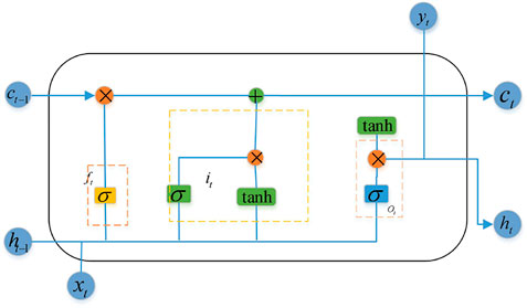
FIGURE 1. The structure of LSTM-based neuron.

LSTM is designed from storage cells that store long-term dependencies. The LSTM cell structure is shown in Figure 1, in addition to the storage unit, the LSTM cell also contains an input gate $i_t$, an output gate $o_t$ and a forget gate $f_t$, the core computing node (Cell), used to record the state information of the cell at the current moment.

The unwanted information in the LSTM is identified and discarded from the cell state through the sigmoid layer defined as the forgetting gate layer. The gate will read $h_{t-1}$ and $x_t$ output a value between 0 and 1 for each cell state. 0 means “completely discarded” and 1 means “completely retained.” Represents the output of the previous cell, and $h_{t-1}$ represents the input of the current cell.

The new information stored in the cell state is determined and updated by a sigmoid layer called the input gate layer. Next, the tanh layer creates a new candidate value vector that can be added to the state.

Update the previous layer of cells $c_{t-1}$ as $c_t$, the cell state is updated as follows,

4) Finalize what values need to be output, this value depends on my cell state, will run a sigmoid layer to decide which parts of the cell state will be exported. The cell state is then treated with tan h (giving a value between [-1,1]) and multiplied it by the output of the sigmoid to get the part we determine the output.

One-way LSTM models use previous information to predict subsequent information, while BILSTM can comprehensively learn both forward and backward time-related information to improve prediction accuracy. In PV power forecasting, considering that information about the past and the future in PV power time series data can play an important role at the same time, we also used BILSTM for simulation experiments to compare with LSTM. BILSTM models include both the forward LSTM layer and the backward LSTM layer. In the forward cell unit, the sequential input layer is the data, obtaining the first set of state output $\left\{h_1\mathrm{,}{h}_2\mathrm{...}\mathrm{,}{h}_k\right\}$, in the reverse cell unit, the data of the input layer is entered in reverse order to obtain the second set of state output $\left\{h_k\mathrm{,}{h}_{k-1}\mathrm{...}\mathrm{,}{h}_1\right\}$, the two sets of states are imported Spliced into $\left[h_1\mathrm{,}{h}_1\right]\left[h_2\mathrm{,}{h}_2\right]$, ..., $\left[h_k\mathrm{,}{h}_k\right]$, and finally $x_t$ gets the input corresponding to the state output is $H_t=\left[h_t\mathrm{,}{h}_t\right]$. The structure diagram of BILSTM is shown in Figure 2.

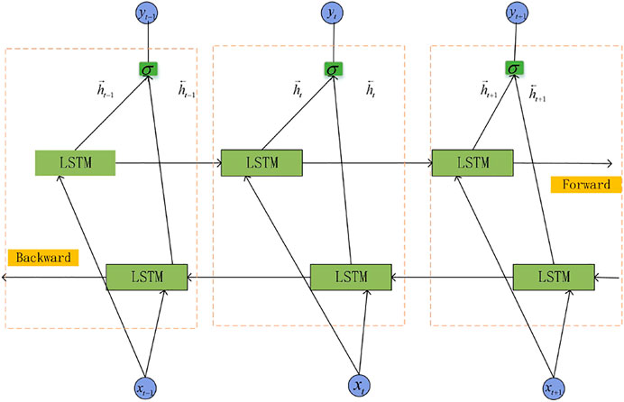
FIGURE 2. BILSTM model structure.

3.3 WOA-BILSTM Model

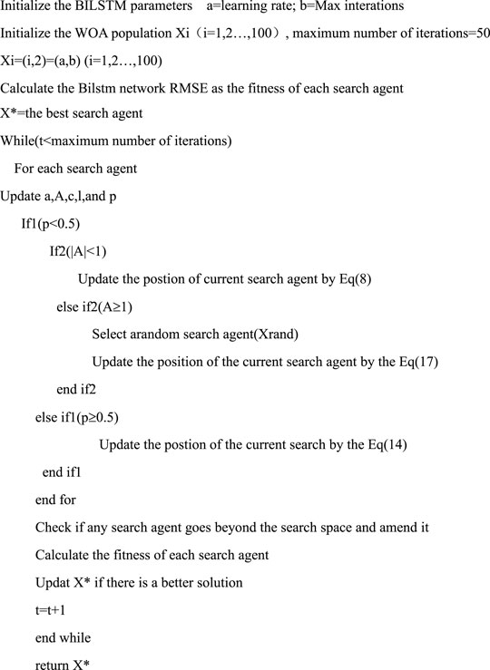
The prediction accuracy of the BILSTM model is mainly affected by the learning rate and the maximum number of iterations. However, the manual selection of the learning rate and the maximum number of iterations is a huge workload and it is difficult to find the optimal parameters, resulting in poor prediction accuracy. Therefore, using WOA to optimize the learning rate and the maximum number of iterations of BILSTM, the combined WOA-BILSTM model is obtained as shown in Figure 3.

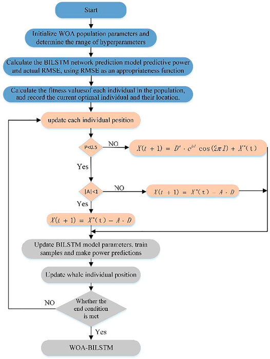
FIGURE 3. Optimization process of the WOA-BILSTM model.

4 Photovoltaic Output Power Prediction Model

4.1 PPF Model Based on FCM-WOA-BILSTM

Based on the theory of appeal, this paper constructs the PPF model of FCM-WOA-BILSTM and its prediction flow Figure 4, the whale optimization algorithm has good optimization ability, excellent global convergence effect, and fast convergence speed. Since the learning rate and the maximum number of iterations are determined in the BILSTM training, it is often necessary to select human experience in order to avoid the difference in human experience affecting the prediction effect of the BILSTM model. In this paper, the whale optimization algorithm is proposed to optimize the learning rate and the maximum number of iterations of the model.

FIGURE 4. FCM-WOA-BILSTM model prediction flow chart.

In the actual forecasting process, we will first read the corresponding data set from the SCADA system, and due to the existence of “garbage data” in a large number of light-voltage datasets, the data will first be cleansed, including the interpolation and rejection of missing and outlier values. The modeling steps are:

Step 1. Data processing of raw photovoltaic power data, including the filling of missing values and the treatment of outliers, excluding “garbage data” that is inconsistent with actual production, and then normalizing the data due to the different dimensions of each variable.

Step 2. The daily maximum, minimum, and average irradiation intensity; the maximum, minimum, and average temperature; and the maximum, minimum, and average wind speed are taken as the feature vectors reflecting the daily.

Step 3. The dimension of the data obtained in step 2 is reduced by PCA, the main factors affecting the photovoltaic output are selected by the PCA algorithm, and the dimension of the original high-dimensional data is reduced to facilitate the visualization of two-dimensional data.

Step 4. The data reflecting the daily eigenvectors after dimensionality reduction are clustered by FCM, and the daily eigenvector data set is divided into four categories according to the weather type: sunny, cloudy, rainy, and extreme weather divide each type of data sample that is well clustered into training sets and test sets.

Step 5. Initialize the dimensions, number of iterations, and population number of WOA. The range of values for parameters that determine the learning rate and the maximum number of iterations.

Step 6. Bring the divided four sets of training sets to the WOA-BILSTM model for training, and take the root mean square error between the predicted value of the photovoltaic power and the actual value of the model as the WOA the fitness value, calculating the corresponding fitness of each population, using the smallest fitness value as the optimization result, comparing it with the globally optimal result, updating the optimal population location as well as the minimum fitness value.

Step 7. Start iterating, using the WOA algorithm to update the two parameters corresponding to the population, repeat step 7 and 8 until the iteration is complete. Outputs the learning rate and the maximum number of iterations corresponding to the final optimal result for each model.

Step 8. By calculating the European-style clustering of the day to be predicted and the center of clustering, the weather type of the day to be predicted is determined, and the corresponding model is substituted to obtain the corresponding photovoltaic forecast power, RMSE, and MAE.

The flow of FCM-WOA-BILSTM photovoltaic power prediction model is shown in Figure 4.

4.2 Error Evaluation Index

In order to better compare the prediction effects of each model, three error evaluation criteria including mean absolute error (MAE), root mean square error (RMSE), and determining coefficient ($R^2$) are used to analyze the feasibility and effectiveness.

$P_t^{act}$ is the actual measured value of the output power of the photovoltaic power station at time t (MW); $P_t^{pre}$ is the predicted value of output power (MW) of a photovoltaic power station at time t; $P_{total}$ is the installed capacity of the photovoltaic power station (130 MW); $P_t^{ave}$ is the average value of actual power; Is n is the total number of samples.

5 Case Analysis

For the historical data of a 130 MW installed capacity photovoltaic power station in 2019, the sampling interval is 15 min. Using BP, GRU, LSTM, BILSTM, PSO-BILSTM, FCM-PSO-BP, and FCM-WOA-LSTM models for short-term PPF, the error of the prediction result is compared and analyzed from various angles.

5.1 Experimental Data Preprocessing

The data cleaning of the sampling data of photovoltaic power generation are carried out. Firstly, the abnormal data with the photovoltaic output of 0 and the irradiation intensity of 0 are eliminated. The key research time is 07:30–17:30, and the sampling interval is 15 min. Due to the small difference between sunrise and sunset every day, there are about 40 strongholds every day, and the missing values are supplemented by interpolation, then the box bitmap is used to eliminate the abnormal data. Each group of data includes four environmental data variables: total irradiation intensity, air temperature, air pressure, and relative humidity from 07:30 to 17:30 every day, as well as photovoltaic power data. Finally, 15,770 groups of experimental data are obtained. In order to eliminate the noise in the time series data and reduce the complexity of the data, the input of the acquired time-series data is subject to component analysis to obtain two-dimensional data with strong representativeness. The data samples were clustered by FCM to classify the samples into four categories: sunny, cloudy, rainy, and extreme weather.

5.2 Short-Term PV Power Forecast Based on Similar Days of FCM-WOA-LSTM

Based on similar daily clustering, combined with the WOA-BILSTM neural network, this paper establishes a short-term prediction model of FCM-WOA-LSTM photovoltaic output power, and the main implementation steps are as follows:

Determine the basic structure of the BILSTM neural network, determine the inputs and outputs of the training samples, and the structural parameters and hyperparameters of the neural network, and use the initial learning rate and the maximum number of iterations of the BILSTM neural network as particles in the WOA algorithm. The WOA optimizes the hyperparameters of the BILSTM network to establish a preliminary WOA-BILSTM basic model.

The forecast day in the test set is randomly selected, and the daily feature vector corresponding to the selected forecast day is determined. The weather type of the forecast day is determined through the Euclidean Distance measurement between the forecast day and each cluster center. The samples in the weather type category of the forecast day are extracted and brought into the WOA-BILSTM model for training. After meeting the conditions, the training is ended and the model is established.

In order to verify the effectiveness of the proposed FCM and WOA in improving the accuracy of short-term photovoltaic power prediction of the basic model of bidirectional long-term and short-term memory network. Take 14 June 2019 (sunny), 18 July 2019 (cloudy), and 22 June 2019 (rainy) as the forecast days, and verify them through three models: BILSTM, FCM-BILSTM, and FCM-WOA-BILSTM. The prediction results for 14 June 2019 (sunny), 18 July 2019 (cloudy), and 22 June 2019 (rainy) are shown in Figures 5–7, respectively.

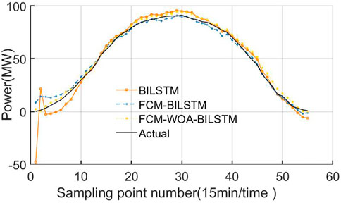
FIGURE 5. 14 June 2019 (sunny).

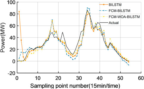
FIGURE 6. 18 July 2019 (cloudy).

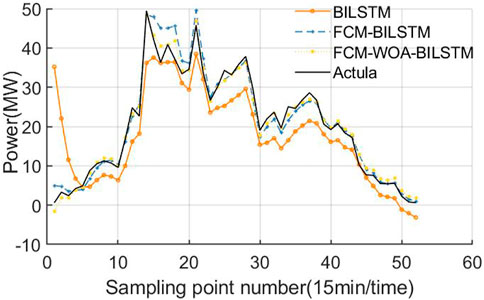
FIGURE 7. 22 June 2019 (rainy).

It can be seen from Figure 5 that under the condition of sunny weather, the power fluctuation range is small, and the prediction error of BILSTM basic model in the initial stage of sampling on that day is too large. After adding FCM clustering algorithm, the prediction error of FCM-BILSTM in the initial sampling stage of the day is relatively improved. On this basis, the prediction error of FCM-WOA-BILSTM model after introducing the WOA algorithm is significantly reduced in the initial sampling stage of the day.

As can be seen from Figure 6, in cloudy weather, the power fluctuation is relatively large, and there are large errors in the basic BILSTM model at each prediction time of the day, especially in the initial stage of sampling on the day. FCM- BILSTM has significantly improved the prediction of the initial sampling stage of the day compared with BILSTM, but there is still a large error between the prediction data of the whole day and the actual sampling data. The prediction results of FCM-WOA-BILSTM model perform well in the initial sampling stage of the day, and the prediction data accuracy of the sampling points within the whole day (with large fluctuation at the 16th sampling point) is very high.

It can be seen from Figure 7 that under rainy weather conditions, BILSTM model has the same problem of low accuracy in the initial stage of sampling on that day, and the prediction error is generally large for the whole day. Compared with BILSTM model, FCM- BILSTM model has improved the prediction accuracy, and FCM-WOA-BILSTM model has significantly improved the prediction effect and high accuracy at each sampling point. Combined with the prediction curves of various models under various weather types, it can be seen that FCM-WOA-BILSTM model has significantly improved the prediction accuracy of BILSTM basic model, with small error fluctuation and good prediction effect.

Table 1 shows the underlying BILSTM model selected and the introduction of FCM and WOA Schematic diagram of the algorithm’s FCM-BILSTM and FCM-WOA-BILSTM models predicting performance in various weather types.

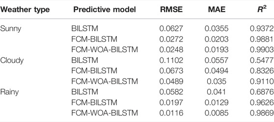
TABLE 1. Error index of three models.

As can be seen from Table 1, on sunny days, the RMSE of the BILSTM, FCM-BILSTM, and FCM-WOA-BILSTM models are 0.0627, 0.0272, and 0.0248, respectively, and the MAEs are 0.0355, 0.0203, and 0.0193, respectively. It shows that the prediction accuracy of each model is higher under the sunny weather type. The introduction of the FCM algorithm on the BILSTM model reduces the RMSE by 0.0355 and the MAE by 0.0152 on the basis of the original high accuracy, demonstrating the effectiveness of the intervention of the FCM algorithm for photovoltaic power prediction. Introducing WOA on the basis of FCM-BILSTM, its RMSE and MAE are further reduced, which effectively proves the practicability of WOA in optimizing BILSTM hyperparameters under sunny days. At the same time, on a sunny day, the $R^2$ of BILSTM was as high as 0.9372 and increased to 0.9881 after the introduction of FCM. On the basis of FCM-BILSTM, the WOA algorithm was added to optimize the hyperparameters of BILSTM, and $R^2$ was further increased to 0.9903. It can effectively improve the stability of photovoltaic power prediction. In cloudy conditions, the RMSE of BILSTM, FCM-BILSTM, and FCM-WOA-BILSTM models are 0.1102, 0.0673, and 0.0489, respectively, and the MAE are 0.0557, 0.0494, and 0.035, respectively, indicating that in cloudy weather with relatively large power fluctuations, the FCM and the WOA algorithm greatly improve the accuracy of the prediction model. Compared with the BILSTM model, the FCM-WOA-BILSTM reduces the RMSE by 0.0613 and the MAE by 0.0207, demonstrating that the FCM and WOA algorithms can effectively improve the prediction accuracy of the BILSTM model in rainy weather. After the introduction of FCM and WOA, its $R^2$ increased from 0.5477 to 0.9110, which proved that FCM and WOA algorithms can effectively improve the stability of photovoltaic power prediction in rainy conditions.

In the rainy season, the RMSE of the BILSTM、FCM-BILSTM, and FCM-WOA-BILSTM models are 0.0582, 0.0197, and 0.0116, respectively, and the MAE are 0.041, 0.0129, and 0.0085, respectively. It can be seen that on rainy days with large power fluctuations, compared with BILSTM, FCM-BILSTM reduces RMSE by 0.0385 and MAE by 0.0281, indicating that FCM is effective in improving photovoltaic power prediction accuracy on rainy days, while FCM-WOA-BILSTM compared with the FCM-BILSTM model, the RMSE and MAE of the model are further reduced, which proves the feasibility of WOA to optimize BILSTM on rainy days. The $R^2$ of FCM-BILSTM and FCM-WOA-BILSTM are 0.9626 and 0.9869, respectively, demonstrating that FCM and WOA algorithms can effectively improve the stability of photovoltaic power prediction on rainy days.

To sum up, under various weather types, both WOA and FCM algorithms can effectively improve the accuracy and stability of photovoltaic short-term power prediction.

In order to further verify the universality and superiority of the short-term photovoltaic power prediction model proposed in this paper, the prediction performance of the FCM-WOA-BILSTM model and other neural network models is compared to the sunny weather with small power fluctuations and the cloudy and rainy weather with large power fluctuations. Figures 8–10 show the power prediction curve of each model under different weather types, and Table 2 shows the RMSE, MAE, and $R^2$, each model under various weather types comparison results of the three evaluation indicators.

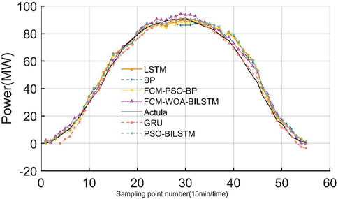
FIGURE 8. 14 June 2019 (sunny).

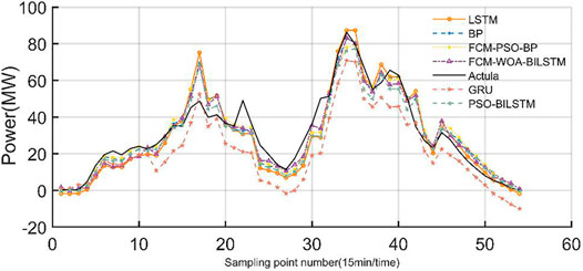
FIGURE 9. 18 July 2019 (cloudy).

FIGURE 10. 22 June 2019 (rainy).

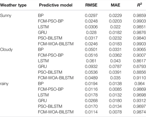
TABLE 2. Error index of four models.

As can be seen from Figures 8–10, the FCM-WOA-BILSTM model proposed in this paper has high prediction accuracy and good performance in various weather types. On sunny days when the output power is relatively stable, the energy concentration of each model predicts the power output situation better.

It can be seen from Table 2 that its RMSE is below 0.031 and the $R^2$ above 0.985. Compared with FCM-PSO-BP model with high prediction accuracy, the model proposed in this paper is basically the same in RMSE and $R^2$, but has an improvement of 0.002 in Mae, indicating that the prediction effect of this model is better under the condition of high accuracy. When the output power fluctuates greatly (on cloudy and rainy days), there is a certain deviation between the prediction curve of each model and the real power curve, and the prediction effect is lower than that on sunny days. The prediction effect of LSTM model and BP model is poor.

FCM-PSO-BP model and the model proposed in this paper are very stable in various evaluation indexes, in which FCM-WOALSTM remains above 0.91 in $R^2$. The cloudy world is as high as 0.9869, and the robustness of the model has been at a high level. It can be seen from the figure that under the sunny weather type, the prediction effect of each model is better than that of the cloudy and rainy weather types, and the prediction error of the FCM-WOA-LSTM model proposed in this paper is smaller than that of other models. The above results show that the FCM-WOA-LSTM model prediction has higher prediction accuracy and can better generate electricity for optical volts under different weather types.

5.3 Posterior-Variance Test

Set the actual value of the t-moment to be $P_t^{act}$ and the predicted value to $P_t^{pre}$, ${\overline{P}}_{act}$ is the average value of the actual value of the test set power, e(t) is the residual error at time t, and its average value is $\overline{\text{e}}$:

Suppose the variance of the original data is the square of S₁, the variance of the residual is the square of S₂, then:

The posterior difference ratio C = $\frac{S_2}{S_1}$, the small error frequency $P=P\{e\left(t\right)-\overline{e}|\le 0.6745S_1\}$ , and the indicators C and P can be used to test the prediction and fitting effect of the model. For prediction with good generalization ability, the index C must be very small, because the value of C is small, indicating that $S_1$ is large and $S_2$ is small, $S_1$ is large, indicating that the observed data has a large dispersion, and the original data has poor regularity, and $S_2$ is small, indicating that the dispersion of the prediction error is small, and the swing range of the prediction error is small. Small error probability P, the larger the p value, the more points where the difference between the residual and the mean value of the residual is less than 0.6745 $S_1$, indicating that the residual is relatively close and the prediction fitting effect is good. According to the P and C values, the model prediction accuracy is divided into four categories (Table 3).

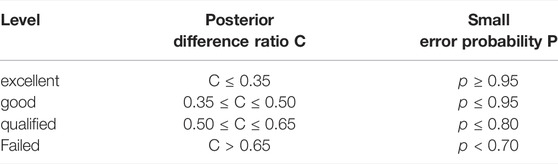
TABLE 3. Reference values of the evaluation level.

The posterior difference method was used to test the FCM-WOA-BILSTM model, and the accuracy of the model was tested with the prediction results of three different weather types, and the test results were obtained in Table 4.

TABLE 4. Results of the evaluation level.

It can be seen from Table 4 that on 14 June 2019 (Sunny), the posterior difference ratio C = 0.056 is obtained, and the small error probability P = 1, so the prediction accuracy level on sunny days is excellent. On 18 July 2019 (Cloudy), the posterior difference ratio C = 0.230 and the small error probability p = 0.967 were obtained, so the prediction accuracy level in cloudy was excellent. On 22 June 2019 (rainy), the posterior difference ratio C = 0.164 was obtained, and the small error probability P = 1, so the prediction accuracy level in rainy was excellent.

Through the post-error test of the power prediction results under different weather types, it can be seen that the prediction accuracy grades are excellent, which further verifies the universality of the FCM-WOA-BILSTM model under various weather types.

6 Uncertainty Analysis of PPF

6.1 Non-Parametric Kernel Density Estimation

Accurate uncertainty analysis of photovoltaic power prediction is of great significance for grid scheduling. In the uncertainty analysis of this study, NPKDE and confidence intervals were used to reflect the error distribution of the PPF. NKPDE is different from PDE in that it does not need to know the data distribution in advance, and it is more practical. In this study, the Gaussian kernel function is selected as the kernel function of NPKDE.

6.2 Calculation Analysis

6.2.1 Probability Density Estimation of PPF Error

Determining the probability density distribution characteristics of the error is the premise of using the confidence interval to calculate the distribution range of the actual value of photovoltaic power. The NPKDE method in Section was used to calculate the probability density distribution of sunny, cloudy, and rainy. Figure 11 is the probability density distribution of PPF.

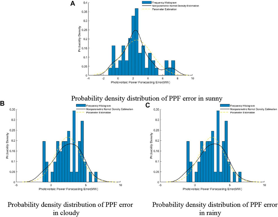
FIGURE 11. Probability density distribution of PPF.

As shown in Figure 11, the histogram represents the distribution of the PPF error, the yellow dotted line is the probability density distribution of the PPF error obtained by the parameter estimation method, and the black solid line represents the probability density distribution of the PPF error obtained by the NPKDE method. The figure shows that, compared with the parameter estimation method, the probability density curve obtained by the NPKDE method can more accurately describe the distribution characteristics of the PPF error.

After the probability density distribution of the PPF error was obtained, the uncertainty distribution of the PPF was quantified using confidence intervals. Figures 12–15 shows the distribution of confidence intervals at 97.5%, 95%, 90%, and 85% confidence levels for different weather conditions of the FCM-WOA-BILSTM prediction model. In Figures 12–15, the solid yellow line represents the PV power forecast value obtained by the FCMWOA-BILSTM method, and the solid black line represents the actual PV power.

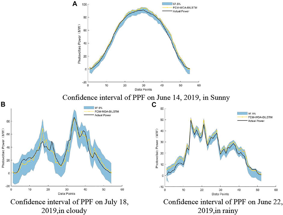
FIGURE 12. 97.5% Confidence interval of PPF under different climatic conditions.

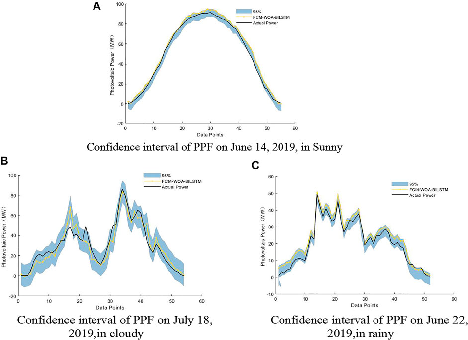
FIGURE 13. 95% Confidence interval of PPF under different climatic conditions.

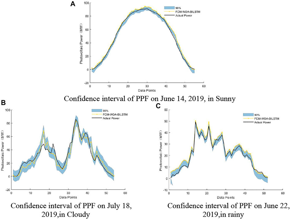
FIGURE 14. 90% Confidence interval of PPF under different climatic conditions.

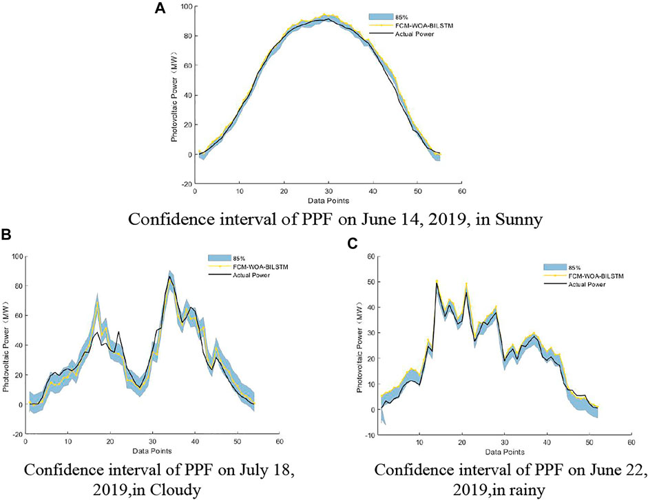
FIGURE 15. 85% Confidence interval of PPF under different climatic conditions.

The results show that under different weather conditions, a small part of the actual value of photovoltaic power is not within the confidence interval due to other potential factors, including NWP error, photovoltaic power plant failure, and shutdown. However, most actual values of photovoltaic power are still within the confidence interval with a probability greater than the confidence level.

Table 5 shows the coverage of PPF confidence intervals based on the FCM-WOA-BILSTM model under different meteorological conditions. The coverage of the PPF confidence interval is above the confidence level. This confirms that using the NPKDE method to quantify the confidence interval can accurately describe the distribution range of the actual power output of photovoltaic power generation.

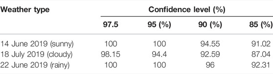
TABLE 5. Coverage rate of confidence interval.

Uncertainty analysis of PPF is an important strategy to promote photovoltaic power consumption and improve grid stability. Based on the photovoltaic power generation of the FCM-WOA-BILSTM model, this study proposes to use NPKDE to quantify the power error distribution. It can be seen from the interval coverage (PCIP) table that the NPKDE algorithm can accurately calculate the FCM-WOA-BILSTM model. prediction error distribution.

7 Conclusion

Aiming at the problem that the accuracy and universality of photovoltaic power short-term prediction models under different weather types are difficult to balance, this paper proposes an optimized neural network hybrid model combined with similar daily clustering. To accurately calculate the probability density distribution of forecasting error, the NPKDE method is used to calculate the probability density distribution characteristics of forecasting error, and the confidence interval and coverage rate of day-ahead PPF. The key findings are as follows:

(1) The prediction effect of BILSTM model under different weather types is different. In this paper, the FCM algorithm based on similar days is used to cluster photovoltaic historical data, and four types of similar-day sample sets are obtained. It is proved that using the FCM algorithm to classify weather can effectively improve the prediction accuracy of the model.

(2) The WOA is used to optimize the hyperparameters of the bidirectional long-short-time memory network and, compared with the optimization algorithms such as PSO and GA, the WOA algorithm has stronger optimization performance. Compared with a single BILSTM model, the prediction effect is significantly improved.

(3) Under different weather types, the RMSE and MAE are lower than other models in the paper, which proves that the prediction accuracy of the FCM-WOA-BILSTM model is relatively high, and $R^2$. It is above 0.985 on sunny and cloudy days, reflecting the high prediction stability of the model.

(4) The NPKDE method is found to describe the probability density distribution characteristics of the PPF error with greater relative accuracy compared to the parametric method.

The combinatorial model proposed in this paper is more complex and cannot take into account the predicted accuracy and prediction speed. Future studies could fruitfully explore this issue further by reducing the loops of the program and changing it to vector operations and through improvements to optimization algorithms. Strive to achieve the highest possible speed of calculation without losing the accuracy of prediction.

Data Availability Statement

The original contributions presented in the study are included in the article/Supplementary Material; further inquiries can be directed to the corresponding authors.

Author Contributions

QX, corresponding author, is primarily responsible for this article. WC was instrumental in the selection of research topics and funding support for this paper. JLZ analyzed the work and wrote the first draft of the manuscript. JZ made a significant contribution to the data processing and analysis of this article. All authors participated in the revision of the manuscript and read and approved the submitted version.

Funding

This work was supported in part by Academic Degrees & Graduate Education Reform Project of Henan Province (2021SJGLX078Y), the Key Scientific Research Projects Plan of Henan Higher Education Institutions under Grant 19A470006, and Cultivation Plan of Young Backbone Teachers in Colleges and Universities of Henan Province under Grant 2019GGJS104.

Conflict of Interest

The authors declare that the research was conducted in the absence of any commercial or financial relationships that could be construed as a potential conflict of interest.

Publisher’s Note

All claims expressed in this article are solely those of the authors and do not necessarily represent those of their affiliated organizations, or those of the publisher, the editors, and the reviewers. Any product that may be evaluated in this article, or claim that may be made by its manufacturer, is not guaranteed or endorsed by the publisher.

References

Almonacid, F., Pérez-Higueras, P. J., Fernández, E. F., and Hontoria, L. (2014). A Methodology Based on Dynamic Artificial Neural Network for Short-Term Forecasting of the Power Output of a PV Generator. Energy Convers. Manag. 85, 389–398. doi:10.1016/j.enconman.2014.05.090
Bian, H., Zhong, Y., Sun, J., and Shi, F. (2020). Study on Power Consumption Load Forecast Based on K-Means Clustering and FCM-BP Model. Energy Rep. 6, 693–700. doi:10.1016/j.egyr.2020.11.148
Changwei, L., Jinghua, L., Bo, C., Yujin, H., and Shanyang, W. (2019). Review of Photovoltaic Power Output Prediction Technology. Trans. china el ect rotechnical Soc. 34 (6), 1201–1217. doi:10.19595/j.cnki.1000-6753.tces.180326
Du, B., Huang, S., Guo, J., Tang, H., Wang, L., and Zhou, S. (2022). Interval Forecasting for Urban Water Demand Using PSO Optimized KDE Distribution and LSTM Neural Networks. Appl. Soft Comput. 122, 108875. doi:10.1016/j.asoc.2022.108875
Duan, J., Wang, P., Ma, W., Tian, X., Fang, S., Cheng, Y., et al. (2021). Short-term Wind Power Forecasting Using the Hybrid Model of Improved Variational Mode Decomposition and Correntropy Long Short -term Memory Neural Network. Energy 214, 118980. doi:10.1016/j.energy.2020.118980
Elmagbri, F., and Mnatsakanov, R. M. (2018). Nonparametric Density Estimation Based on the Scaled Laplace Transform Inversion. Trans. A. Razmadze Math. Inst. 172 (3), 440–447. doi:10.1016/j.trmi.2018.09.003
Fei, Y., Zong, X., Qiao, Y., and Wang, Q. (2016). Photovoltaic Power Prediction Technology. Power Syst. Autom. 40 (04), 140–151. doi:10.7500/AEPS20150711003
Ge, L., Xian, Y., Yan, J., Wang, B., and Wang, Z. (2020). A Hybrid Model for Short-Term PV Output Forecasting Based on PCA-GWO-GRNN. J. Mod. Power Syst. Clean Energy 8 (6), 1268–1275. doi:10.35833/MPCE.2020.000004
Gharehchopogh, F. S., and Gholizadeh, H. (2019). A Comprehensive Survey: Whale Optimization Algorithm and its Applications. Swarm Evol. Comput. 48, 1–24. doi:10.1016/j.swevo.2019.03.004
Guang, Z., Lu, L., Tang, B., Wang, S., Yang, X., and Chen, R. (2021). An Improved Hybrid Neural Network Ultra-short-term Photovoltaic Power Forecasting Meth Od Based on Cloud Image Feature Extraction. Proc. CSEE (20), 6989–7003. doi:10.13334/j.0258-8013.pcsee.201929
Hu, J., Wang, J., and Xiao, L. (2017). A Hybrid Approach Based on the Gaussian Process with T-Observation Model for Short-Term Wind Speed Forecasts. Renew. Energy 114, 670–685. doi:10.1016/j.renene.2017.05.093
Hu, W., and Zhang, B. (2018). Short-term Wind Power Forecast Based on Back-Propagation Neural Network Corrected by Markov Chain. Euro. J. Electric. Engineer. 20 (3), 279–293. doi:10.3166/ejee.20.279-293
Jiang, W., Zhao, Y,, Wang, B,, Feng, S., Pei, Y., and Zhang, F. (2021). Photovoltaic Power Prediction Method Based on NWP Irradiance Inclination Conversion. J. Shandong Univ. Eng. Sci. 51 (05), 114–121. doi:10.6040/j.issn.1672-3961.0.2020.104
Jin, Y., Jiang, H., Qiang, Y., Li, J., Wang, Q., Ru, J., et al. (2021). China's Photovoltaic Industry 2020 Review and 2021 Outlook. Sol. Energy (04), 42–50. doi:10.19911/j.1003-0417.tyn20210304.b
Li, G., Wang, H., Zhang, S., Xin, J., and Liu, H. (2019). Recurrent Neural Networks Based Photovoltaic Power Forecasting Approach. Energies 12 (13), 2538. doi:10.3390/en12132538
Liu, H., Chen, D., Lin, F., and Wan, Z. (2021). Wind Power Short-Term Forecasting Based on LSTM Neural Network with Dragonfly Algorithm. J. Phys. Conf. Ser. 1748, 032015. doi:10.1088/1742-6596/1748/3/032015
Liu, L., Zhao, Y., Chang, D., Xie, J., Ma, Z., Sun, Q., et al. (2018). Prediction of Short-Term PV Power Output and Uncertainty Analysis. Appl. energy 228, 700–711. doi:10.1016/j.apenergy.2018.06.112
Liu, Y., and Liu, L. (2021). Wind Power Prediction Based on LSTM-CNN Optimization. Sci. J. Intelligent Syst. Res. 3 (4), 277–285.
López Gómez, J., Ogando Martínez, A., Troncoso Pastoriza, F., Febrero Garrido, L., Granada Álvarez, E., and Orosa García, J. A. (2020). Photovoltaic Power Prediction Using Artificial Neural Networks and Numerical Weather Data. Sustainability 12 (24), 10295. doi:10.3390/su122410295
Lv, J., Zheng, X., Pawlak, M., Mo, W., and Miśkowicz, M. (2021). Very Short-Term Probabilistic Wind Power Prediction Using Sparse Machine Learning and Nonparametric Density Estimation Algorithms. Renew. Energy 177, 181–192. doi:10.1016/j.renene.2021.05.123
Ma, T., Yang, H., and Lu, L. (2014). Solar Photovoltaic System Modeling and Performance Prediction. Renew. Sustain. Energy Rev. 36, 304–315. doi:10.1016/j.rser.2014.04.057
Mayer, M. J., and Gróf, G. (2021). Extensive Comparison of Physical Models for Photovoltaic Power Forecasting. Appl. Energy 283, 116239. doi:10.1016/j.apenergy.2020.116239
Shang, Z., He, Z., Song, Y., Yang, Y., Li, L., and Chen, Y. (2020). A Novel Combined Model for Short-Term Electric Load Forecasting Based on Whale Optimization Algorithm. Neural Process Lett. 52 (2), 1207–1232. doi:10.1007/s11063-020-10300-0
Singh, P. K., Singh, N., and Negi, R. (2021). Short-term Wind Power Prediction Using Hybrid Auto Regressive Integrated Moving Average Model and Dynamic Particle Swarm Optimization. Int. J. Cognitive Inf. Nat. Intell. (IJCINI) 15 (2), 111–138. doi:10.4018/IJCINI.20210401.oa9
Sugiyama, S. (2007). Forecast Uncertainty and Monte Carlo Simulation. Foresight Int. J. Appl. Forecast. 6 (6), 29–37.
Sun, M., Feng, C., and Zhang, J. (2020). Multi-distribution Ensemble Probabilistic Wind Power Forecasting. Renew. Energy 148, 135–149. doi:10.1016/j.renene.2019.11.145
Takamatsu, T., Ohtake, H., and Oozeki, T. (2022). Support Vector Quantile Regression for the Post-Processing of Meso-Scale Ensemble Prediction System Data in the Kanto Region: Solar Power Forecast Reducing Overestimation. Energies 15 (4), 1330. doi:10.3390/en15041330
Tuerxun, W., Xu, C., Guo, H., Guo, L., Zeng, N., and Gao, Y. (2022). A Wind Power Forecasting Model Using LSTM Optimized by the Modified Bald Eagle Search Algorithm. Energies 15 (6), 2031. doi:10.3390/en15062031
Von Loeper, F., Schaumann, P., de Langlard, M., Hess, R., Bäsmann, R., and Schmidt, V. (2020). Probabilistic Prediction of Solar Power Supply to Distribution Networks, Using Forecasts of Global Horizontal Irradiation. Sol. Energy 203, 145–156. doi:10.1016/j.solener.2020.04.001
Wang, L., Liu, Y., Li, T., Xie, X., and Chang, C. (2020). Short-term PV Power Prediction Based on Optimized VMD and LSTM. IEEE Access 8, 165849–165862. doi:10.1109/ACCESS.2020.3022246
Wang, M. (2018). The Prediction of Photovoltaic Power Output Based on the Extreme Learning Machine Algorithm of Particle Swarm Optimization. Int. J. Comput. Eng. 1 (1), 100–102.
Wu, X., Wang, H.-Y., Shi, P., Sun, R., Wang, X., Luo, Z., et al. (2022). Long Short-Term Memory Model - A Deep Learning Approach for Medical Data with Irregularity in Cancer Predication with Tumor Markers. Comput. Biol. Med. 144, 105362. doi:10.1016/j.compbiomed.2022.105362
Xie, X., Zhou, J., Zhang, Y., Wang, J., and Su, J. (2020). W-BiLSTM Based Ultra-short-term Generation Power Prediction Method of Renewable Energy. Autom. Electr. Power Syst. 45 (08), 175–184. doi:10.7500/AEPS20200718002
Yan, J., Liu, Y., Han, S., Wang, Y., and Feng, S. (2015). Reviews on Uncertainty Analysis of Wind Power Forecasting. Renew. Sustain. Energy Rev. 52, 1322–1330. doi:10.1016/j.rser.2015.07.197
Zhao, X., Ge, C., Ji, F., and Liu, Y. (2021). Monte Carlo Method and Quantile Regression for Uncertainty Analysis of Wind Power Forecasting Based on Chaos-LS-SVM. Int. J. Control Autom. Syst. 19 (11), 3731–3740. doi:10.1007/s12555-020-0529-z
Keywords: fuzzy c-means clustering, whale optimization algorithm, BiLSTM, photovoltaic power forecasting, uncertainty analysis
Citation: Cao W, Zhou J, Xu Q, Zhen J and Huang X (2022) Short-Term Forecasting and Uncertainty Analysis of Photovoltaic Power Based on the FCM-WOA-BILSTM Model. Front. Energy Res. 10:926774. doi: 10.3389/fenrg.2022.926774
Received: 23 April 2022; Accepted: 24 May 2022;
Published: 07 July 2022.
Edited by:
Peng Hou, Independent Researcher, Aarhus, DenmarkReviewed by:
Jie Shi, University of Jinan, ChinaHuiling Chen, Wenzhou University, China
Yongquan Zhou, Guangxi University for Nationalities, China
Copyright © 2022 Cao, Zhou, Xu, Zhen and Huang. This is an open-access article distributed under the terms of the Creative Commons Attribution License (CC BY). The use, distribution or reproduction in other forums is permitted, provided the original author(s) and the copyright owner(s) are credited and that the original publication in this journal is cited, in accordance with accepted academic practice. No use, distribution or reproduction is permitted which does not comply with these terms.
*Correspondence: Qiang Xu, xuqiang@ncwu.edu.cn; Junlong Zhou, Z20201050598@stu.ncwu.edu.cn