Green Building Energy Cost Optimization With Deep Belief Network and Firefly Algorithm

Introduction

The building industry is one of the largest sectors in creating jobs and has made great impact on the economy. Meanwhile, the buildings consume large amounts of natural resources such as water and electricity and its adverse environmental impacts are widely concerned. According to the World Business Council for Sustainable Development, buildings has contributed to more than 40% of total energy consumption (Mull, 1998) and 30% of greenhouse has emission (Payne et al., 2012). As a result, the high energy cost and environmental impacts from the buildings are becoming a major issue (Li et al., 2021a).

The new concept Green Building (GB) is conceived as an opportunity to reduce adverse impacts of buildings on the environment and energy cost. GB has been defined as a term that is interchangeable with buildings that has efficient energy utility and high sustainability. An increasing number of studies have been conducted on GB in the past decade and one major research direction is the reduction of the energy cost. Heating, ventilation, and air-conditioning (HVAC) systems are the major source of energy consumption in commercial buildings, and they account for more than 60% of annual total energy utility.

Previous literature has invested significant research efforts related to the modeling and optimization of the HVAC systems. They can be classified into two types of approaches: the physics-based approaches and the data-driven approaches. Physics-based approaches are generally developed over mathematical equations to depict the HVAC system modules and have been extensively utilized in HVAC related research. Sakulpipatsin et al. (2010) proposed extended physics-based models of HVAC systems and used TRNSYS software to perform the simulation for optimization studies. Zhang et al. (2013) introduced a novel physics-based model to study the HVAC energy consumption mechanism and a new model parameter namely entrants is included in the model. Teodosiu et al. (2003) developed an analytical model to evaluate thermal comfort by considering indoor air moisture and its transport by the airflow. Nassif et al. (2004) proposed a supervisory control strategy to optimize set points of controllers used in a multi-zone HVAC system.

The physics-based approaches are usually computationally complex and can be only applied under certain conditions. In comparison, data-driven approaches have reflected effectiveness in modeling complex, dynamic, and non-linear systems in many domains (He et al., 2017; He and Kusiak, 2017; Ouyang et al., 2017; Li et al., 2018; Ouyang et al., 2018; Li et al., 2020). Kusiak et al. (2011a) proposed a data-mining approach for the optimization of the HVAC units. Chang et al. (2009) constructed a Hopfield neural network to model the chilled water supply temperatures in chillers. Fong et al. (2006) used TRNSYS software to construct a data-driven model to optimize the settings of chilled water and supply air temperature. Lv et al. (2018) discussed various low carbon technologies and strategies to optimize the green building HVAC energy consumption. Kontes et al. (2013) proposed a stochastic optimization algorithm to maximize the utility of renewable energy proportion within the HVAC system. Lachheb et al. (2020) studied parametric models to investigate the impact of HVAC utility on the glazing size in various regions. Promising results from the data-driven approaches have demonstrated the effectiveness and robustness in modeling and optimizing the HVAC systems.

Inspired by the recent advent of deep learning algorithms, in this research, we would like to advocate a novel data-driven framework to modeling and optimizing the energy cost. In this modeling stage, the artificial neural network is constructed and trained on the HVAC energy consumption dataset to study the non-linear mapping between input features and energy cost. The algorithm with the top performance is selected as the benchmark for the following stage. In stage II, a firefly algorithm is utilized as the optimizer to reduce the total energy consumption while maintaining the air quality at an acceptable level.

HAVC System and Problem Formulation

HVAC System

HAVC systems are widely installed in the commercial buildings located in the central business district (CBD). A schematic diagram of a typical HVAC system installed in the commercial buildings is illustrated in Figure 1. A typical HVAC system consists an air handling unit (AHU) and multiple thermal zones. For each thermal zone, a VAV (variable air volume) box is connected to the air handling unit to maintain the comfort temperature of the thermal zone.

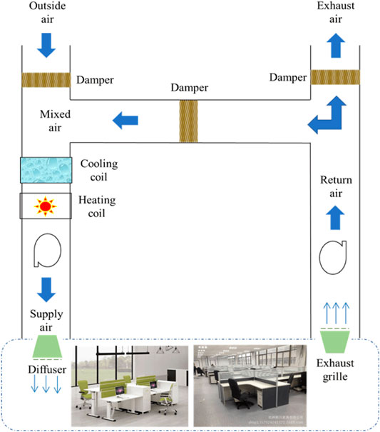
FIGURE 1. Schematic diagram of an HVAC system.

The total energy utility by the HVAC system is consisted of the utility from the AHU and VAV. Three major resources including heat energy, fan energy, and pump energy, account for all energy consumptions in the AHU. For the VAV, the reheat load accounts for the maximum consumed energy (Kusiak et al., 2011b). The VAV box basically supplied the conditioned air for a specific thermal zone in order to satisfy the comfort temperature of the zone envelope. By tuning the dampers in the VAV box, the hot water flows through the coils adjusting to the actual requirements of the zone comfort.

Data Collection

The HVAC system discussed in this research as our case study is operated by a commercial building located in the central business district in Chengdu, China. This building has 33 floors and many big companies set their regional headquarter offices inside this building.

The dataset provided contains the hourly data of the HVAC system in the underlying building during the whole year of 2019. Multiple features that are relevant to our study is provided including total energy consumption, supply air temperature set point, supply air duct static pressure set point, system load, supply air humidity, barometric pressure, and outside air temperature. The in-detail description of the features utilized in this study has been summarized in Table 1 as follows.

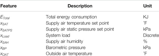
TABLE 1. Introduction of the related features collected in the dataset.

Problem Formulation

In this research, the main goal is to develop a data-driven framework to minimize the total energy cost which ensuring the indoor air quality is maintained at a desirable level. The setting of the two controllable parameters namely the supply air temperature set point and the supply air static pressure set point play the essential role in impacting the total energy consumption of the HVAC system.

The total energy utility of an HVAC system comes from the AHU and VAV and it can be expressed in eq. 1 as follows:

Based on prior domain knowledge, the input features are associated with the AHU and VAV and we may re-formulate the problem as a regression problem as expressed in eq. 2:

Among them, the $x_{SAT}$ and the $x_{SATPS}$ are controllable features and the rest are uncontrollable features.

In this research, the goal is to reduce the energy consumption while maintaining the indoor air quality. Hence, according to literature review (Kusial et al., 2011; Li et al., 2021b), we set the following constrains to our optimization model: the supply air temperature ($x_{SAT}$) should be between 50°F and 65°F; the supply air duct static pressure ($x_{SATPS}$) must be between 0.2 and 0.5 kPa; and the supply air humidity ($x_{SAH}$) should be controlled below 25%. Consequently, it can be formulated in the following non-linear optimization problem with the underlying constraints in eq. 3 as follows:

subject to:

Methodology

Deep Belief Network

The number of applications of deep learning architecture in regression, multi-class classification, collaborative filtering, and graphic learning tasks has experienced rapid growing in the recent decade (LeCun et al., 2015). In this section, a deep-learning based framework is presented to predict wind direction. The concept of deep learning originates from research on artificial neural networks and it alleviates the local optima problem in the non-convex objective function of a neural network (Ouyang et al., 2020). The success of deep learning architectures is contributed by three characteristics: a large number of hidden neurons, better learning algorithms, and better parameter initialization techniques (Deng and Yu, 2013).

In this paper, a widely utilized deep-learning algorithm namely deep belief network (DBN) is selected to construct the regression models to predict total energy consumption of the HVAC system. Originally proposed by Hinton et al. (2006), a typical DBN contains multiple restricted Boltzmann machines (RBMs) which are stacked in a hierarchically manner. Each RBM includes a visible layer and a hidden layer both are composed of Boolean neurons (see Figure 2). The connection between the hidden layer and the visible layer is bidirectional and symmetrical without any inter-connections between neurons in the same layer exists.

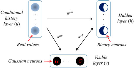
FIGURE 2. Restricted Boltzmann Machine (RBM).

The optimization of the weight matrix between the two layers is the main target in the training process in order to construct a robust mapping. The configuration of weight matrix is based on the energy function expressed in eq. 4 (Hinton et al., 2006). The joint distribution of a visible layer vector and the hidden layer vector is expressed in eq. 5. The activation functions of neurons in the visible and hidden layer are presented in eqs. 6, 7 (Hinton et al., 2006):

Layer-wise Training

Multiple layers of restricted Boltzmann machines (RBMs) are hierarchically stacked within the DBN algorithm. The first RBM is pre-trained as an independent RBM and the weight matrix of the first RBM is computed. The output of the first RBM is treated as the input to the second RBM. By training the RBMs iteratively following the above strategy, the DBN is trained and the weight matrices between the remaining hidden layers are obtained.

During the training process of RBMs, the optimization problem is formulated using a stochastic gradient ascent approach (SGA) (Hinton et al., 2006). Based on vector (5) of the joint distribution function between the visible and hidden layer, the objective function of the stochastic gradient ascend method is expressed in eq. 8:

Benchmarking Algorithms

Three benchmarking algorithms including support vector regression machine (SVR), neural network (NN), and extreme learning machine (ELM).

The support vector regression machine (SVR) is a supervised classification/regression algorithm that includes a Gaussian kernel function (Drucker et al., 1996). The neural network (NN) is a machine-learning algorithm which contains the input layer, hidden layer and the output layer. The extreme learning machine (ELM) algorithm (Liang et al., 2006) is a single hidden layer feedforward network. The ELM learning model is expressed in eqs. 9, 10 (He and Kusiak 2017; Li et al., 2018; Ouyang et al., 2019; Li et al., 2021c).

Firefly Algorithm

The Firefly Algorithm (FA) (Bacanin et al., 2021) is a new swarm intelligence algorithm that simulates the social behavior of fireflies. In the nature, fireflies use flashing to attract mating partners and the movement of the fireflies is determined by the resulting attraction which is related to the intensity of the emitted light. Similar to the particle swarm optimization (PSO) algorithm, the FA algorithm is a population-based stochastic search algorithm. Each firefly member in the population represents a candidate solution in the search space. Fireflies move toward other directions and search potential candidate solutions. Overall, the attractiveness is determined by the intensity of the emitted light that is measured by the fitness value (Wang et al., 2017).

In detail, the attractiveness between the two fireflies X_i and X_j can be computed in eqs. 11, 12 as follows:

where d = 1,2,3, … ,D and D is the problem dimension; r_ij is the distance between X_i and X_j; x_id and x_jd are the dimension of X_i and X_j respectively. Each firefly X_i is compared with all other fireflies X_j, where j = 1,2, … ,N and $j\ne i$. If X_j is brighter than X_i, the X_i will be attracted by X_j and move towards X_j. The movement of X_i can be computed by eq. 13 as follows:

Therefore, the FA algorithm can be summarized into the following three steps as follows:

• Step 1: Initialization. Randomly generate N solutions as an initial population accordingly. Each individual solution (firefly) is $X_i$.

• Step 2: Movement (attraction). For each solution $X_i$, we compare with all other solutions $X_j$. If $X_j$ is greater than $X_i$, $X_i$moves towards $X_j$ and changes its position according to eq. 13.

• Step 3: Stopping. If the stopping criteria has been satisfied, we can stop the algorithm.

Measurement Metrices

In this research, the prediction output is the energy consumption and hence we may formulate this as a regression problem. Two widely utilized metrics namely mean absolute percentage error (MAPE) and root mean square error (RMSE) are selected in this study to measure the performance of different DBN architectures (Li et la. 2021b). The MAPE and RMSE are expressed in eq. 8, 9 as follows:

Experimental Results

Feature Analysis

In this research, the HAVC energy consumption dataset includes six predictor variables (features) and the energy utility is the dependent variable as indicated in Section “Data Collection”. All features are continuous numerical features and the feature preliminary analysis with min-max scaling and histogram are performed in this section.

As illustrated in Figure 4, the histograms of the energy consumption are presented. In order to investigate the energy consuming behavior of the underlying commercial building in different seasons, the hourly energy consumption in summer season (Jun-Aug) and winter season (Dec-Feb) has been randomly sampled and plotted in Figure 3. It is obvious that the two energy distributions are right-skewed and are non-Gaussian distributed.

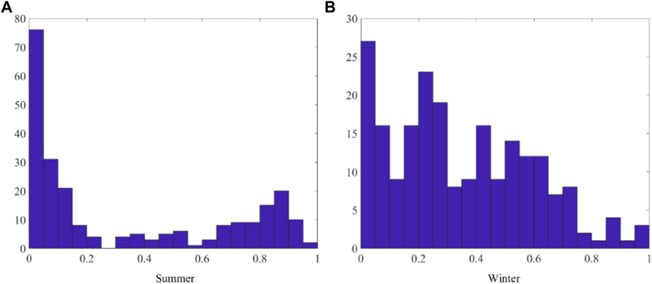
FIGURE 3. Histogram of energy consumption in summer and winter.

Meanwhile, the histograms of the input predictor features are also illustrated in Figure 4 as follows. From Figure 4, almost all predictors follow a Gaussian-type of distribution and are symmetric in their empirical PDFs. The only exception is SAPTS which is left-skewed which indicate it may follow a non-Gaussian distribution. A log-transformation will be applied to further transform the distribution into a Gaussian shape distribution.

FIGURE 4. Histogram of predictor variables.

Predictive Modeling of Energy Cost

After data-preprocessing, the predictive modeling of energy consumption using DBN is provided in this section. The two hyper-parameters, the number of RBMs and the number of neurons within each RBM, directly impact the predicting performance of the energy prediction model. Hence, it is essential to tune the hyper-parameters to ensure the optimal setting of the DBN algorithm.

In this research, a cross-validation based tuning process is implemented. As illustrated in Figure 5, we performed a series of experiments testing the average RMSE of various hidden layers as well as various hidden neurons in each hidden layer using an incremental manner. The dataset for such experiment are randomly sampled from the original dataset which contains a whole month hourly energy consumption records. It is obvious that the optimal number of RMBs within the DBN is 2 and the optimal number of hidden neurons in each RMB is 15.

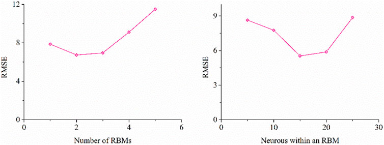
FIGURE 5. Hyper-parameter tuning process.

Using the constructed optimal DBN algorithm, we performed training and testing experiments on two seasons: summer and winter. In each experiment, a whole month dataset has been used as the training dataset and the following weekly data has been used as the validation dataset. The prediction performance has been illustrated in Figure 7 respectively. The prediction results of the testing dataset contain the actual energy consumption (blue) and the predicted energy consumption (red) of the two seasons. In summer, the RMSE is 5.51, and the MAPE is 11.77%. In winter, the RMSE is 5.25 and the MAPE is 10.81%. The prediction performance of the trained DBNs as well as the benchmarking machine learning algorithms on the testing dataset is presented in Table 2 and Figure 6 respectively.

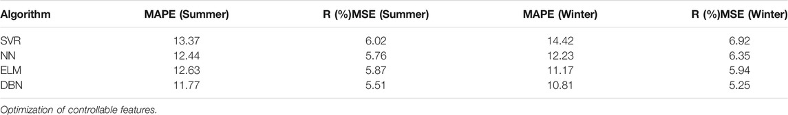
TABLE 2. Prediction performance of all algorithms tested.

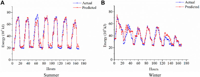
FIGURE 6. Prediction performance of the testing dataset in Summer and Winter.

In this section, the optimization of controllable features namely the supply air temperature set point (SAT) and the supply air static pressure set point (SATPS) in the temporal domain has been optimized by using the constructed DBN prediction models. The goal of the optimization is to reduce the energy consumption while maintaining the indoor quality. The formulation is expressed in eq. 3 and the constrains for all predictor features are listed to ensure the indoor air quality. The firefly algorithm (FA) has been implemented in this section to reduce the energy consumption and the optimization experiments is illustrated in Figure 7 as follows.

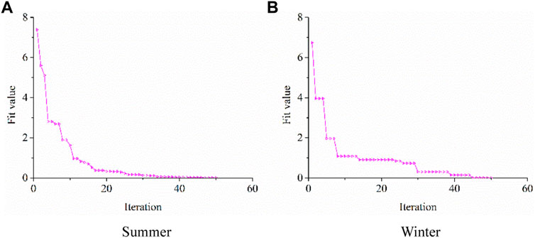
FIGURE 7. Optimization experiment of firefly algorithm.

As illustrated in Figure 7, the fitness value of the FA algorithm has been plotted along with the iteration of the experiments. For the summer prediction model, the fitness value converges to near-zero zone after 20 epochs indicating the optimal solution has been numerically approached. For the winter prediction model, the fitness value converges to near-zero region after 30 epochs as it achieved its optimal solution. As it takes more epochs to approach the optimal solution, it indicates more complexity in the winter prediction model due to the challenges within the dataset provided.

Hence, using the feature settings computed by the FA algorithm, the two optimized feature outcomes are selected as new inputs in the pre-trained energy prediction models as discussed in Section “Predictive modeling of energy cost”. The simulation results are presented in Figure 8 that contains the actual energy consumption (blue), predicted energy consumption (red), and optimized energy consumption (purple) computed from the simulation outcome. For the summer season, the simulation results indicate the optimized energy consumption is 17% less than the predicted energy utility. For the winter season, the optimized energy is 14% less than the predicted energy utility.

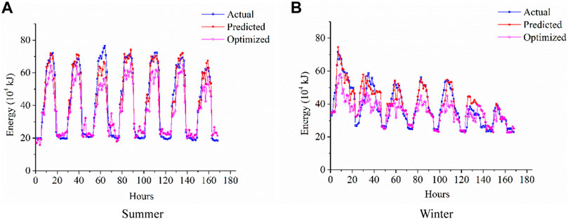
FIGURE 8. Simulated energy consumption using the optimized controllable feature setting.

Based on the simulation results, we have achieved an optimized energy utility in our testing dataset. Considering the local electricity price, and total area within our underlying building, we have achieved a cost saving of 12.90 RMB/m² for our case study building in summer and 11.18 RMB/m² in winter from an economic perspective. If we incorporate this into the estimation of the total energy cost of the whole building, it would approximately achieve 16.6% of reduction in the total cost considering the savings in both winter and summer. Therefore, it achieved the standard Green Building concept and can be utilized as a sample for other local commercial buildings for larger scale energy saving projects.

Conclusion

The best performing neural network structure has been selected via cross-validation and gird-based search. In addition, an energy optimization problem has been formulated by incorporating the predictive neural network model and HVAC operational constraints. The formulated optimization problem has been successfully solved by the firefly algorithm. The optimal setting of the two controllable features including the supply air temperature set point and the supply air static pressure set point in the temporal domain has been computed. Computational results demonstrated that it can achieve the reduction of total energy cost by a significant portion. (Wang et al., 2016).

Data Availability Statement

The original contributions presented in the study are included in the article/Supplementary Material, further inquiries can be directed to the corresponding author.

Author Contributions

YL conceptualized the study, contributed to the study methodology, and wrote the original draft. YL contributed to the study methodology, data curation and investigation. CC contributed to data analysis and investigation. LZ contributed to investigation and writing-original draft. All authors have read and agreed to the published version of the manuscript.

Conflict of Interest

The authors declare that the research was conducted in the absence of any commercial or financial relationships that could be construed as a potential conflict of interest.

Publisher’s Note

All claims expressed in this article are solely those of the authors and do not necessarily represent those of their affiliated organizations, or those of the publisher, the editors and the reviewers. Any product that may be evaluated in this article, or claim that may be made by its manufacturer, is not guaranteed or endorsed by the publisher.

References

Glossary

$E_{Total}$ Total energy consumption

$E_{AHU}$ Energy utility from the AHU

$E_{VAV}$ Energy utility from the VAV

$x_{SAT}$ Supply air temperature set point

$x_{SATPS}$ Supply air duct static pressure

$x_{Load}$ System load

$x_{SAH}$ Supply air humidity

$x_{BP}$ Barometric pressure

$x_{OAT}$ Outside air temperature.

vi Number of neurons in the visible layer

hi Number of Boolean neurons within the hidden layer

wj,I Weight matrix between the visible layer and hidden layer

ai Weight vector connecting the ith hidden node and the input nodes

bi Threshold of the ith hidden node

sig() Logistic sigmoid function

a Bias vector of the visible layer

b Bias vector of the hidden layer

xj Input parameters

oj Output values

fL() Non-linear function representing the ELM algorithm

βi Weight vector connecting the ith hidden node and the output nodes

tj Actual output value

${\mathit{ϵ}}_i$ Random value uniformly distributed between [-0.5, 0.5]

s Step-factor between [0, 1]

$\widehat{y_i}$ Predicted value

$y_i$ Actual value

$N$ Total number of predicted values in the testing dataset

References

Bacanin, N., Bezdan, T., Venkatachalam, K., and Al-Turjman, F. (2021). Optimized Convolutional Neural Network by Firefly Algorithm for Magnetic Resonance Image Classification of Glioma Brain Tumor Grade. J. Real-time Image Proc. 18, 1085–1098. doi:10.1007/s11554-021-01106-x
Chang, Y.-C., and Chen, W.-H. (2009). Optimal Chilled Water Temperature Calculation of Multiple Chiller Systems Using Hopfield Neural Network for Saving Energy. Energy 34 (4), 448–456. doi:10.1016/j.energy.2008.12.010
Deng, L., and Yu, D. (2013). Deep Learning for Signal and Information Processing. Microsoft Res. Monogr..
Drucker, H., Burges, C. J., Kaufman, L., Smola, A., and Vapnik, V. (1996). Support Vector Regression Machines. Adv. Neural Inf. Process. Syst. 9, 155–161.
Fong, K. F., Hanby, V. I., and Chow, T. T. (2006). HVAC System Optimization for Energy Management by Evolutionary Programming. Energy and Buildings 38 (3), 220–231. doi:10.1016/j.enbuild.2005.05.008
He, Y., Deng, J., and Li, H. (2017). Short-term Power Load Forecasting with Deep Belief Network and Copula Models. Proceeddings of the 9th International conference on intelligent human-machine systems and cybernetics (IHMSC). 26 August. 2017. Hangzhou, China, 1. IEEE, 191–194. doi:10.1109/ihmsc.2017.50
He, Y., and Kusiak, A. (2017). Performance Assessment of Wind Turbines: Data-Derived Quantitative Metrics. IEEE Trans. Sustainable Energ. 9 (1), 65–73.
Hinton, G. E., Osindero, S., and Teh, Y.-W. (2006). A Fast Learning Algorithm for Deep Belief Nets. Neural Comput. 18 (7), 1527–1554. doi:10.1162/neco.2006.18.7.1527
Kontes, G. D., Giannakis, G. I., and Rovas, D. (2013). Demand Shifting Using Model-Assisted Control. Int. J. Energ. a Clean Environ. 14 (1). doi:10.1615/interjenercleanenv.2014007281
Kusiak, A., Tang, F., and Xu, G. (2011a). Multi-objective Optimization of HVAC System with an Evolutionary Computation Algorithm. Energy 36 (5), 2440–2449. doi:10.1016/j.energy.2011.01.030
Kusiak, A., Xu, G., and Tang, F. (2011b). Optimization of an HVAC System with a Strength Multi-Objective Particle-Swarm Algorithm. Energy 36 (10), 5935–5943. doi:10.1016/j.energy.2011.08.024
Lachheb, A., Allouhi, A., Saadani, R., Jamil, A., and Miloud, R. A. H. M. O. U. N. E. (2020). Thermal and Economic Analysis of Different Glazing Systems for a Commercial Building in Various Moroccan Climates. Int. J. Energ. a Clean Environ. 22.
LeCun, Y., Bengio, Y., and Hinton, G. (2015). Deep Learning. Nature 521 (7553), 436–444. doi:10.1038/nature14539
Li, H., Deng, J., Feng, P., Pu, C., Arachchige, D. D. K., Cheng, Q., et al. (2021b). Monitoring and Identifying Wind Turbine Generator Bearing Faults Using Deep Belief Network and EWMA Control. Front. Energ. Res. 9, 799039. doi:10.3389/fenrg.2021.799039
Li, H., Deng, J., Feng, P., Pu, C., Arachchige, D. D. K., and Cheng, Q. (2021a). Short-Term Nacelle Orientation Forecasting Using Bilinear Transformation and ICEEMDAN Framework. Front. Energ. Res. 9, 780928. doi:10.3389/fenrg.2021.780928
Li, H., He, Y., Yang, H., Wei, Y., Li, S., and Xu, J. (2021c). Rainfall Prediction Using Optimally Pruned Extreme Learning Machines. Nat. Hazards 108 (1), 799–817. doi:10.1007/s11069-021-04706-9
Li, H., Xu, Q., He, Y., and Deng, J. (2018). Prediction of Landslide Displacement with an Ensemble-Based Extreme Learning Machine and Copula Models. Landslides 15 (10), 2047–2059. doi:10.1007/s10346-018-1020-2
Li, H., Xu, Q., He, Y., Fan, X., and Li, S. (2020). Modeling and Predicting Reservoir Landslide Displacement with Deep Belief Network and EWMA Control Charts: a Case Study in Three Gorges Reservoir. Landslides 17 (3), 693–707. doi:10.1007/s10346-019-01312-6
Liang, N.-Y., Saratchandran, P., Huang, G.-B., and Sundararajan, N. (2006). Classification of Mental Tasks from EEG Signals Using Extreme Learning Machine. Int. J. Neur. Syst. 16 (01), 29–38. doi:10.1142/s0129065706000482
Lv, Y., Bi, J., and Yan, J. (2018). State-of-the-art in Low Carbon Community. Int. J. Energ. a Clean Environ. 19 (3-4). doi:10.1615/interjenercleanenv.2018025415
Nassif, N., Kajl, S., and Sabourin, R. (2004). Evolutionary Algorithms for Multi-Objective Optimization in HVAC System Control strategyIEEE Annual Meeting of the Fuzzy Information. Process. NAFIPS 04 (1), 51–56. doi:10.1109/nafips.2004.1336248
Ouyang, T., He, Y., and Huang, H. (2018). Monitoring Wind Turbines' Unhealthy Status: A Data-Driven Approach. IEEE Trans. Emerging Top. Comput. Intelligence 3 (2), 163–172.
Ouyang, T., He, Y., Li, H., Sun, Z., and Baek, S. (2019). Modeling and Forecasting Short-Term Power Load with Copula Model and Deep Belief Network. IEEE Trans. Emerg. Top. Comput. Intell. 3 (2), 127–136. doi:10.1109/tetci.2018.2880511
Ouyang, T., Huang, H., He, Y., and Tang, Z. (2020). Chaotic Wind Power Time Series Prediction via Switching Data-Driven Modes. Renew. Energ. 145, 270–281. doi:10.1016/j.renene.2019.06.047
Ouyang, T., Kusiak, A., and He, Y. (2017). Predictive Model of Yaw Error in a Wind Turbine. Energy 123, 119–130. doi:10.1016/j.energy.2017.01.150
Payne, F. W., and McGowan, J. J. (2012). Energy Management and Control Systems Handbook. Springer Science & Business Media.
Sakulpipatsin, P., Itard, L. C. M., Van der Kooi, H. J., Boelman, E. C., and Luscuere, P. G. (2010). An Exergy Application for Analysis of Buildings and HVAC Systems. Energy and buildings 42 (1), 90–99. doi:10.1016/j.enbuild.2009.07.015
Teodosiu, C., Hohota, R., Rusaouën, G., and Woloszyn, M. (2003). Numerical Prediction of Indoor Air Humidity and its Effect on Indoor Environment. Building Environ. 38 (5), 655–664. doi:10.1016/s0360-1323(02)00211-1
Wang, H., Wang, W., Zhou, X., Sun, H., Zhao, J., Yu, X., et al. (2017). Firefly Algorithm with Neighborhood Attraction. Inf. Sci. 382-383, 374–387. doi:10.1016/j.ins.2016.12.024
Wang, H. Z., Wang, G. B., Li, G. Q., Peng, J. C., and Liu, Y. T. (2016). Deep Belief Network Based Deterministic and Probabilistic Wind Speed Forecasting Approach. Appl. Energ. 182, 80–93. doi:10.1016/j.apenergy.2016.08.108
Zhang, L., Liu, X., and Jiang, Y. (2013). Application of Entransy in the Analysis of HVAC Systems in Buildings. Energy 53, 332–342. doi:10.1016/j.energy.2013.02.015