Updated geostrophic circulation and volume transport from satellite data in the Southern Ocean

1 Introduction

The ocean is subject to a variety of physical forces, including gravity, friction, pressure gradient, and the Coriolis force. The Coriolis force, in particular, is an inertial force that acts within a rotating frame of reference. In the Southern Hemisphere, this force acts to the left of the velocity direction within a reference frame with clockwise rotation, but in the Northern Hemisphere, it acts to the right within an anticlockwise rotating reference frame. The balance between the pressure gradient and the Coriolis force gives rise to the geostrophic currents (GCs), which are the most important component in ocean circulation and play a critical role in shaping Earth’s climate system.

When studying the GC of the Southern Ocean, the Antarctic Circumpolar Current (ACC) emerges as the predominant current. The ACC is the world’s most powerful ocean current, flowing eastward around Antarctica and linking the Atlantic, Pacific, and Indian oceans. The ACC plays a fundamental role in global ocean circulation by linking the major ocean basins and substantially contributing to heat and water transport. Consequently, accurately estimating the transport of the ACC is critical for comprehending and simulating Earth’s climate system. However, due to its intricate structure, variability, and remote location, measuring and investigating the ACC is challenging. In recent years, advances in technology and observational techniques have enabled better approximations of the ACC transport, leading to an improved understanding of its dynamics and effects on the global ocean. The ACC was initially characterized as a multi-jet structure, with three primary fronts—the Subantarctic Front (SAF), the Polar Front (PF), and the Southern ACC Front (SACCF)—and two large gyres—the Ross and Weddell gyres (Orsi et al., 1995). However, subsequent research suggests that the ACC is a more complex structure, with additional jets beyond the three classical ones and a third unnamed gyre located between 80°E and 90°E (Sokolov and Rintoul, 2009a; Tarakanov, 2021).

The Drake Passage (DP), situated between Antarctica and South America, is the only region where the ACC is constrained by two continental slopes, linking the Pacific and Atlantic oceans. The DP serves as the most suitable location to investigate the ACC, and numerous monitoring programs have been conducted in this region to estimate its transport. The International Southern Ocean Studies provided data about the current flow in the DP for the first time between the late 1970s and early 1980s. This led to the derivation of the canonical full-depth transport of the ACC at the DP of 134 ± 15 Sv (Whitworth III, 1983; Whitworth III and Peterson, 1985). More recent studies (Cunningham et al., 2003; Firing et al., 2011; Chidichimo et al., 2014; Koenig et al., 2014; Donohue et al., 2016) have estimated the transport across the DP within the range of 136–173 Sv.

In the study by Vigo et al. (2018), it was stated that satellite data have the potential to estimate the three-dimensional (3D) ocean geostrophic circulation with global coverage. Using sea surface height (SSH) data from satellite altimetry and an independent geoid derived from satellite gravity data, specifically from the Gravity field and steady-state Ocean Circulation Explorer (GOCE), the absolute dynamic topography (ADT) is estimated. From the ADT, the partial derivatives along the latitude and longitude are used to determine the velocity field of the surface geostrophic currents (SGCs). These currents are then propagated downwards by considering temperature and salinity profiles based on measurements by Argo floats. The study provided a 3D geostrophy for the Southern Ocean and estimated the associated volume transport (VT) down to a depth of 1,975 m for the period 2004–2014. The zonal ACC and its interaction with a meridional thermohaline circulation were captured, as well the VT of the PF and the SAF fronts of the ACC and the large-scale and mesoscale currents in the Southern Ocean. However, the reported VT at the Drake Passage was slightly overestimated compared to the literature, with values of 185 Sv or 202 Sv (depending on the computation method).

In this study, we aimed to revisit the problem of estimating the 3D GC in the Southern Ocean following the methodology described by Vigo et al. (2018), but including several updates to improve the accuracy and resolution. Specifically, we used updated satellite altimetry and gravity datasets, which have higher spatial and temporal resolution and better coverage than the data used in previous studies. We also incorporated a more recent product for temperature and salinity profiles from the Argo floats and other in situ measurements, which have increased the spatial and temporal coverage of the data, especially at depth.

Using these updated datasets, we were able to provide improved estimates of the 3D geostrophy and VT of the Southern Ocean, covering nearly the full depth. Our results highlight the complex and dynamic nature of the Southern Ocean circulation and provide estimates in good agreement with the literature.

Importantly, our analysis reconciles the different estimates reported in the literature regarding the VT estimates for the DP. Given the global coverage of our study, we were able to provide the VT estimated along the different paths followed in the in situ campaigns in the literature, such as in the studies by Cunningham et al. (2003), Firing et al. (2011), Koenig et al. (2014), Chidichimo et al. (2014), Donohue et al. (2016), and Olivé Abelló et al. (2021). We observed a generally good agreement in most cases, and it was also evident that the estimated VT varied depending on the path followed during the campaigns. By not only validating our results but also reconciling the different VT estimates on the DP provided in the literature, our study provides a comprehensive and updated view of the Southern Ocean circulation and transport.

2 Methodology

Following the same methodology as in the work of Vigo et al. (2018), we estimate the geostrophic flow in the ocean with a synergy of space data. The SGC is computed as the directional derivative of the ADT, which is obtained from satellite data by combining the SSH recovered from altimetry missions and an independent geoid from space gravity missions. Using the SGC as a reference level and a relative dynamic topography (RDT) obtained from temperature and salinity in situ data, we estimate the GC by depths (Wunsch, Gaposchkin,1980).

Thus, we first define the ADT and the RDT as follows:

where $N$ represents a time-averaged geoid, x and y are the longitude and latitude, z is the depth, t is the time, g is the gravitational acceleration (latitude-dependent), P(z) is the pressure at depth z (in Pascal units), and ρ is the water density. The state equation of seawater from the Gibbs Seawater Oceanography Toolbox (McDougall, Barker, 2011) is used to obtain the density from the ocean temperature, salinity, and pressure.

Using the geostrophic equation, i.e., the balance between the pressure gradient force and the Coriolis force at the surface, we calculate the SGC:

where $u_s$ is the zonal surface velocity (positive eastward), $v_s$ is the meridional surface velocity (positive northward), and $f=2\omega \sin \left(y\right)$ is the Coriolis parameter that depends on ω, the average angular rate of Earth’s rotation.

To obtain the value for the GC $u$ and $v$ at any depth $z=z_i$, the SGC is used as a boundary value as follows:

Therefore, using Eqs 3, 4, the GC at depth $z_i$ can be obtained directly from the SGC and the spatial gradients of ADT and RDT (at depth $z_i$):

If we calculate the GC at different depths, we obtain a 3D geostrophic flow. We refer to this 3D estimation of the GC as 3D geostrophy.

Within a cell of a regular grid, the volume of water transported due to the geostrophic flow from the surface to a depth $D$ can be estimated by vertically integrating the 3D geostrophy from that depth to the surface. Note that we must count for the width of the grid cell perpendicular to the transport:

Here, ${VT}_u$ (${VT}_v$) is the zonal (meridional) VT, which is positive eastward (northward), and $w_{NS}$ ($w_{EW}$) is the north–south (east–west) width of the grid cell. Note that in a regular grid, $w_{EW}$ depends on latitude y, whereas $w_{NS}$ is constant. Units of volume transport are Sverdrups (Sv; 1 Sv = 10⁶ m³/s).

To separate the barotropic and baroclinic components of the VT, we adopt the definition given by Fofonoff (1962). That is, we consider the portion of VT due to a water column moving uniformly as fast as the bottom current as barotropic transport and its complementary as baroclinic transport.

3 Data

3.1 Absolute dynamic topography

According to Eq. 1, the ADT is the SSH minus the geoid, where the SSH can be obtained from satellite altimetry data as the sum of the sea level anomalies (SLAs) and the corresponding mean sea surface (MSS):

We can also obtain the mean dynamic topography (MDT) as the difference between the geoid and the MSS:

Then, if the MSS is the same in both SSH and MDT products, we can express the ADT, following (1), (7), and (8), as

In this study, we obtained the ADT using Eq. 9 by utilizing both the MDT and SLA with respect to a common MSS, which is the DTU18MSS high-resolution model generated by the Danish National Space Center. This model is based on 25 years of data collected from multi-mission satellite altimeters, including a 3-year record from Sentinel-3A and an improved 7-year record from Cryosat-2 LM. For further information, please refer to the work of Andersen et al. (2018).

For the MDT, we used the DTUUH19MDT geodetic model developed by the Danish National Space Center. This model makes use of the OGMOG geoid model, which has been augmented using the EIGEN-6C4 coefficients to degree and order 2,160, as well as the aforementioned DTU18MSS mean sea surface model, integrating drifter data to enhance the MDT’s resolution. Refer to the work of Knudsen et al. (2019) for details.

For the SLA, we used the CCI-Sea Level Project (http://www.esa-sealevel-cci.org) product of sea-level maps given as a monthly merged solution from several altimetry satellites (Jason 1 and 2, TOPEX/Poseidon, Envisat, ERS-1 and -2, and GEOSAT-FO) with a spatial resolution of 0.25° for the time span 01/01/1993 to 31/12/2015 (version v2.0, downloaded on December 2019). These maps are anomalies with respect to the same DTU18MSS used for the MDT.

With respect to the work of Vigo et al. (2018), in this study, we utilized updated data to estimate the ADT. Our new approach incorporates a newer geoid model (OGMOG instead of EIGEN-6C3) and an updated SLA solution, which covers a longer time period and is directly referenced to an updated reference MSS (DTU18MSS). Compared to the approach taken by Vigo et al. (2018), our current approach avoids a potential source of error by using the same reference MSS in the calculation of MDT and SLA. In the study by Vigo et al. (2018), SLA was referenced to DTU10MSS, while DTU13MSS was used in the MDT calculation, requiring additional steps to recover the ADT.

3.2 Temperature and salinity profiles

We used the objective analyses EN4.1.1, a quality-controlled subsurface ocean temperature (T) and salinity (S) dataset from the Met Office Hadley Center. These are T and S profiles that include ARGO data and reach 5,500 m depth, which allow us to calculate near full-depth VT. In this product, T and S measurements have been optimally interpolated to a 1°x1° regular grid in 42 depth layers (for further details, see the work of Good et al., 2013). EN.4.1.1 data were obtained from https://www.metoffice.gov.uk/hadobs/en4/ (© British Crown Copyright, Met Office, [2021]) and are provided under a Non-Commercial Government License (http://www.nationalarchives.gov.uk/doc/non-commercial-government-licence/version/2/).

In the study by Vigo et al. (2018), the T and S profiles went from the surface to 2,000 m. In this study, T and S profiles have been extended to near full depth. This extension directly affects the estimates of the full VT, as well as the barotropic and baroclinic VT components.

4 Results and discussion

4.1 3D geostrophic currents

Following Eq. 3, we obtain the SGC from altimetry and gravity space data with 0.25° spatial resolution for the 12 years from 2004 to 2015. Then, we propagate these SGC vector fields, following Eq. 5, to calculate the full-depth 3D GC with monthly time resolution for the same period at 41 levels depths from the surface to 4,900 m depth. The ADT and the surface velocities have been computed with a spatial resolution of 0.25°, whereas for the RDT, we can only provide estimates with 1° spatial resolution due to the T and S data resolution limitation. Therefore, the 3D GC is provided in 1° regular grids.

To visualize our region of interest, in Figure 1A,we display the bathymetry of the SO region and the classical three main ACC fronts (SAF in black, PF in red, and SACCF in green), as described by Orsi et al. (1995) based on hydrological data available until 1990. However, a more recent study by Sokolov and Rintoul (2009b) incorporating both in situ observations and satellite altimetry for the period 1992–2007 reveals a more complex multi-jet structure of the ACC fronts. In Figure 1B, we depict our mean SGC for the SO as black arrows indicating the mean velocity directions overlaid on a colormap that indicates their norm. We also superimpose the multi-jet structure from the study by Sokolov and Rintoul (2009a). Notably, our findings agree remarkably with the latter study, despite the different time period considered in each. Observed jet speeds range from 10 cm/s to 30 cm/s and can reach up to 85 cm/s at the boundary with the Agulhas Current (the colorbar is saturated at 20 cm/s to better visualize results for the entire region).

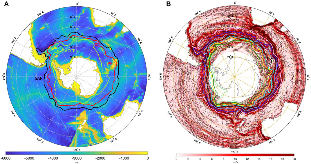
FIGURE 1. (A) Bathymetry in meters from https://download.gebco.net/, with the Southern Ocean fronts from the study by Orsi et al. (1995) indicated by color-coded lines: the Subantarctic Front in black, Polar Front in red, and Southern ACC Front in green. (B) Mean surface geostrophic current velocity for the period 2004–2015, represented by mean direction (black arrows) with background color indicating their norm. For clarity reasons, only the directions for velocities greater than 3 cm/s are represented. Units: cm/s. Color scale saturated at 20 cm/s (maximum values can reach 85 cm/s). The fronts of the ACC described by Sokolov and Rintoul (2009a) are indicated by color-coded lines. From north to south, the Northern, Middle, and Southern jets of the SAF are shown in magenta, dark blue, and lavender, respectively. The Northern, Middle, and Southern jets of the PF are depicted in black, cyan, and yellow, respectively, and the Northern and Southern jets of the SACCF are shown in dark and light green, respectively.

Figures 2, 3 display the time-averaged zonal and meridional velocities, respectively, at different depths. Figure 4 shows the GC speed, which is obtained by computing the Euclidean norm of both velocity components. Note that blank spots increase with depth due to the bathymetry. Figure 2 indicates a dominant eastward component, while Figure 3 depicts an alternation of northward and southward components that correspond to continuous shifts up and down of the eastward ACC fronts and subfronts as they meander. At all depths, the fronts of the ACC and the major currents, including the Agulhas Current, East Australian Current, and Brazil-Malvinas Current, are clearly distinguishable. In Figures 2, 3, the paths of the major ACC middle fronts, as identified by Sokolov and Rintoul (2009a), have been overlaid. It can be observed that along the ACC, the higher velocities in both components follow these fronts and their branches, as shown in Figure 1B for the SGC. This is particularly evident in the zonal component, which reflects the eastward nature of the ACC. However, the intensities of these currents exhibit a decreasing trend with increasing depth. For example, at 0° longitude, the speed of the main fronts decreases for the range from 5 to 968 m at a rate of 0.0053 ± 0.0001 cm/s per meter, 0.0061 ± 0.0001 cm/s per meter, and 0.0021 ± 0.0001 cm/s per meter for the SAF, PF, and SACCF, respectively. When considering the rates of change from 5 m to 2,134 m, the rates for the SAF, PF, and SACCF are 0.0047 ± 0.0001 cm/s per meter, 0.0043 ± 0.0001 cm/s per meter, and 0.0013 ± 0.00008 cm/s per meter, respectively.

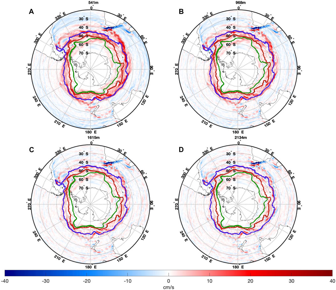
FIGURE 2. Zonal component of the mean geostrophic currents (2004–2015) at depths of (A) 541 m, (B) 968 m, (C) 1,615 m, and (D) 2,134 m. Positive (red) values indicate an eastward direction, while negative (blue) values indicate a westward direction. The units are cm/s, and the values range from −50 cm/s (Agulhas Current near the south of Africa) to 40 cm/s. However, the color scale is saturated at [−40 cm/s, 40 cm/s] to better visualize the interrelation between different depths. The three main jets from the study by Sokolov and Rintoul (2009b) are indicated by color-coded lines: the Middle jet of the SAF is in blue, Middle jet of the PF is in red, and Northern jet of the SACCF is in green.

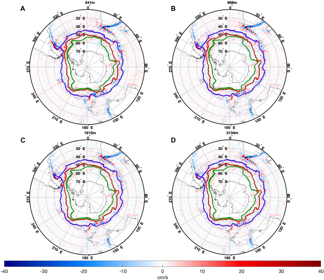
FIGURE 3. Same as Figure 2, but for the meridional component at depths of (A) 541 m, (B) 968 m, (C) 1,615 m, and (D) 2,134 m (color saturated at [−20 cm/s, 20 cm/s]).

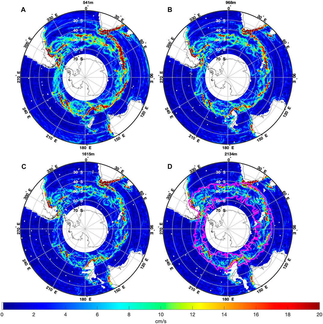
FIGURE 4. Mean geostrophic current speed (2004–2015) at depths of (A) 541 m, (B) 968 m, (C) 1,615 m, and (D) 2,134 m. Units: cm/s. The color scale is saturated at 20 cm/s to better visualize the interrelation between different depths. However, maximum values can reach up to 60 cm/s near the Agulhas Current. (D) The magenta outline indicates the region of the ACC, as defined in Section 4.2.

If we focus on the entire ‘ACC region’, contoured in magenta in Figure 4D, which we will define in the next section based on VT criteria, we obtain a mean (latitude weighted) GC speed (Figure 4) at different depths: 11 ± 0.1 cm/s (5 m), 8.5 ± 0.1 cm/s (540 m), 6.9 ± 0.1 cm/s (967 m), 5.7 ± 0.1 cm/s (1,615 m), and 5.4 ± 0.1 cm/s (2,134 m). In general, we observe a mean speed decrease from 5 m to 2,133 m of 5.6 cm/s, but in areas of maximum intensity, this decrease reaches values up to 25.9 cm/s. This slowdown by depths is almost completely due to the zonal component, with a mean decrease of 6.1 cm/s, while the meridional component stays the same (−0.75 cm/s). Overall, the 3D geostrophy estimates presented in this study are in good agreement with the well-known current pattern of the Southern Ocean.

As already mentioned, the other major Southern Ocean currents are also discernible at all depths from Figures 2–4. In the southwestern Atlantic basin, the Brazil–Malvinas Current Confluence region can be observed. Near South Africa, we observe the Agulhas Current in the western boundary of the southwest Indian Ocean and the Benguela Current in the eastern boundary of the southeast Atlantic Ocean. Starting from south Madagascar, there is a westward current that flows southwest along the east coast of South Africa. From here, two currents emerge, one moving eastward away from the coast and another moving west–north along the western coast of South Africa. Comparing our results with those of the work of Vigo et al. (2018), we observe overall lower intensities, but the ACC and all the other main currents of the Southern Ocean remain depicted. The highest values of speed are reached in the Agulhas Current, with a mean value at the surface of 42.8 cm/s that decreases up to 35.7 cm/s at 968 m, 33.9 cm/s at 1868 m, and 33.6 cm/s at 2,134 m depth.

When compared to previous studies following the same methodology (Vigo et al., 2018), the updated data show slightly lower speeds at the surface and a less-pronounced decrease in these velocities with increasing depth. In figure 4 of the study by Vigo et al. (2018), which is the same as our Figure 4, some points at 500 m depth reach mean speed values of 50 cm/s. In contrast, our results show that almost every point (except for some in the Agulhas Current) has speeds lower than 50 cm/s. These differences are primarily due to the zonal component. In the study by Vigo et al. (2018), zonal GC at 500 m depth reached values up to 60 cm/s; meanwhile, our current estimates show maximum values of 40 cm/s, with the 99th percentile being 21.9 cm/s and the 50th percentile being 2.1 cm/s. This difference in intensity is consistent at all depths.

We interpolated our results to compare with the depths reported by Vigo et al. (2018) for the ACC region and found a mean (latitude-weighted) speed of 11 ± 0.1 cm/s (2.5 m), 8.7 ± 0.1 cm/s (500 m), 6.9 ± 0.1 cm/s (1,000 m), 5.9 ± 0.1 cm/s (1,500 m), and 5.5 ± 0.1 cm/s (1,975 m). Notably, our mean speed near the surface is almost half of the previous results, and at 1,975 m depth, the mean speed is 2.5 times lower. The difference in mean speed between 2.5 m and 1,975 m depth is lower in our results (5.5 cm/s) than that reported by Vigo et al. (2018) (8.4 cm/s).

Vigo et al. (2018) noted that the estimates reported in their study were higher than the estimates found in the literature. This raised concerns about the possible presence of a systematic error in either the methodology or the data used in their study. While we followed the same methodology as in the previous study, the use of updated data has resulted in lower estimates that are more consistent with previous literature, as we will discuss later. It is worth noting that due to the updated datasets used in our study, the defined ACC region in our analysis differs slightly from the one in the study by Vigo et al. (2018).

On the other hand, the estimated meridional component (shown in Figure 3 at different depths) is in closer agreement with previous results reported by Vigo et al. (2018). However, the meridional stripes that were prominent in the previous results are now less discernible. It was previously suggested by Vigo et al. (2018) that these stripes were caused by the assimilation of GRACE data in the used geoid. Due to the polar orbit that GRACE follows, meridional stripes are characteristic of unfiltered GRACE data. However, the use of a more updated geoid in this study appears to have overcome this issue.

4.2 Volume transport

According to Eq. 6, the 3D integrated zonal and meridional VT is obtained by integrating full depth. We also compute the barotropic and baroclinic components for both the zonal and meridional VT. It is important to note that since our approach computes the complete profile up to 4,900 m, the barotropic and baroclinic transport reported here cannot be directly compared with those reported by Vigo et al. (2018), where the reference profile for the barotropic transport was limited to a depth of 1,975 m.

4.2.1 Mean volume transport

In Figure 5, we present two different representations of the time-averaged VT. The mean VT vector is computed by taking the time mean of each component and is represented by black arrows showing the direction, with the colored background representing the norm in Figure 5A. Additionally, we compute a monthly time series of VT vector norms at each grid point, and its time mean is represented in Figure 5B. We refer to this as monthly VT norms. Note the differences between these two representations. If we have 2 months with two opposite vectors with the same magnitude in the same grid point, then 1) the mean VT vector will be null, showing no VT at all; 2) the monthly VT norms will present the norm of the two vectors, that is the mean VT through the grid point in any direction. The monthly VT norms will always be greater than the norm of the mean VT vector.

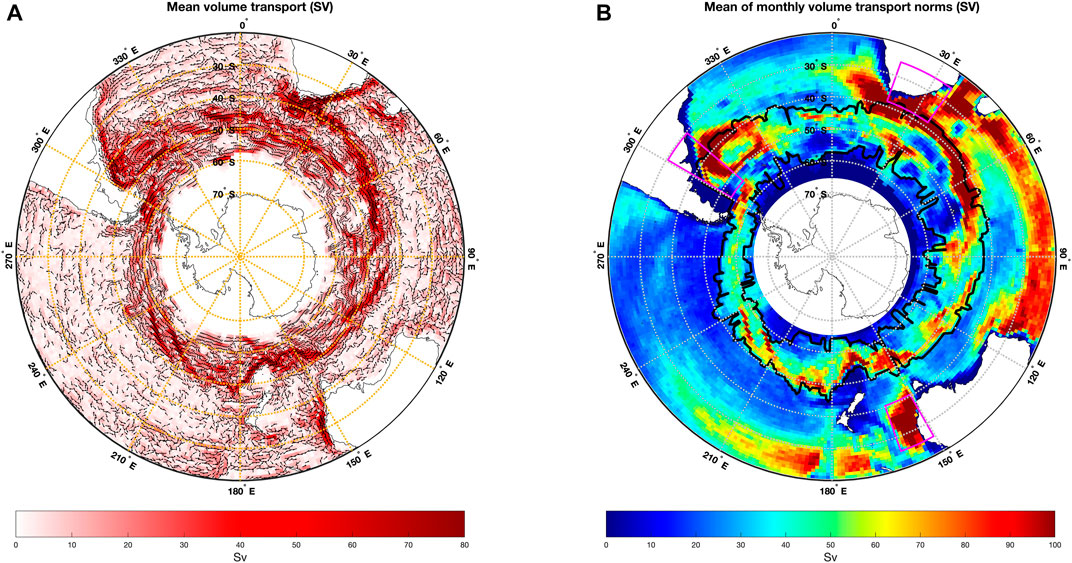
FIGURE 5. Mean geostrophic volume transport (2004–2015): (A) Arrows represent the mean vectors, and the color indicates their norms. Arrows are shown only for mean vectors with a norm greater than 5 Sv to improve clarity. The units are Sv. The color scale is saturated at 80 Sv, and maximum values can reach 300 Sv. (B) Mean of the monthly vector norms. Each grid point has a monthly time series of VT norm, and the mean of this monthly time series is depicted. The units are Sv. The color scale is saturated at 100 Sv, and maximum values can reach 338 Sv. The ACC region (defined as the grid points with a mean zonal volume transport greater than 12 Sv) is outlined in black, and the regions of the Agulhas Current, Brazil–Malvinas Current, and East Australia Currents are outlined in magenta.

We define the ACC region as the grid points in the Southern Ocean that have a mean zonal VT greater than 12 Sv (some outliers have been removed), as depicted by the black outline in Figure 5B. It is important to note that some points with VT higher than 12 Sv are observed outside the ACC region in Figure 5B since this figure shows the mean total VT rather than the mean zonal VT used to define the region.

In Figure 5A, the color scale is set to a maximum value of 80 Sv for better visualization. However, it is important to note that the maximum values can reach as high as 300 Sv and are concentrated in just a few grid points along the Agulhas Current. The 99th percentile is 82.4 Sv. In Figure 5B, the color scale is saturated at 100 Sv. Similar to the previous figure, the highest values can reach up to 338 Sv and are primarily found in the Agulhas Current region. The 95th percentile is 98.5 Sv.

For the subsequent analysis, all reported VT mean values are latitude-weighted mean and refer to Sv per 1° cell. The mean of the VT vector norms in Figure 5A is 8.6 ± 0.1 Sv for the Southern Ocean region. In contrast, the mean of the monthly VT norms (Figure 5B) for the same region is 40.2 ± 0.2 Sv. For the ACC region, the mean of the VT vector norms is 23.7 ± 0.3 Sv, and the mean of the monthly VT norms is 51.7 ± 0.5 Sv. The VT patterns shown in Figure 5A are very similar to those of the SGC (see Figure 1B), with the ACC clearly identified as the dominant current. As with the currents, the transport is primarily driven by the eastward component, with minor north–south shifts due to the meandering of the currents.

In our study, we also analyzed the Brazil–Malvinas Current, the Agulhas Current, and the East Australian Current, which are three of the major currents in the Southern Ocean. Each current region is defined as follows. In the regions outlined in magenta in Figure 5B, each current is defined as the grid points with a mean VT vector norm greater than 100 Sv for the Agulhas Current and greater than 40 Sv for the Brazil–Malvinas Current and the East Australian Current. Both Figures 5A,B depict these major currents.

The Brazil–Malvinas Current originates from the Brazilian coast and flows toward the Brazil-Malvinas Current Islands, located in the region [53.5°S, 30.5°S] x [300.5°E, 310.5°E] in the South Atlantic. This current shows a mean VT vector norm of 65.2 ± 3.2 Sv, which rises to 108.8 ± 5.9 Sv when the monthly VT norms are considered. In the sector [40.5°S] x [302.5°E x 304°E], a previous work by Artana et al. (2018) reported a mean VT of 37.1 ± 6.6 Sv in the upper 1,500 m during 1992–2016. Our updated estimate, on the other hand, yields a slightly higher VT of 47.5 ± 0.6 Sv in the same region and depth range. Notably, despite the difference in time periods, both studies show good agreement.

The Agulhas Current flows southward along the east coast of Africa and is found in the region [38.5°S, 25.5°S] x [19.5°E, 35.5°E] in the Indian Ocean. This current exhibits a mean VT vector norm of 179.1 ± 12.3 Sv, which increases to 217.0 ± 11.8 Sv when monthly VT norms are considered. When we focus on the region [36°S, 33°S] x [26°E, 29°E], as examined by Beal et al. (2015), our method estimates a VT of −81.4 ± 20.5 Sv, which is in close agreement with the value of −84 ± 11 Sv reported by the aforementioned study based on in situ data.

The East Australian Current flows southward along the east coast of Australia and is located in the region [40.5°S, 25.5°S] x [150.5°E, 160.5°E]. This current shows a mean VT vector norm of 61.4 ± 3.3 Sv, which increases to 125.8 ± 7.9 Sv when the monthly VT norms are considered. Our estimate of the meridional transport in the upper 2,000 m (−30.6 ± 6.3 Sv) for the coastal region [27.5°S] x [153.7°E, 155.3°E] is consistent with the −22.1 ± 7.5 Sv reported by Sloyan et al. (2016) for the same period (April 2012 to August 2013).

These results for the Brazil–Malvinas Current, the Agulhas Current, and the East Australian Current are summarized in Table 1. Overall, the agreements with estimates based on in situ data suggest that our estimated VT is robust.

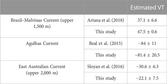
TABLE 1. Comparison between our study and previous studies by different authors for the Brazil–Malvinas Current, Aguhlas Current, and East Australian Current. Units are Sv.

When comparing our updated estimates of mean VT in the ACC, Brazil-Malvinas Current, Agulhas Current, and East Australian Current to those of the work of Vigo et al. (2018), it is clear that our results provide a more detailed pattern of mean VT. Our depiction of ACC fronts also shows greater detail than the previous study. In Figure 5A, our updated estimates are generally consistent with or slightly lower than those obtained using the previous approach. However, in Figure 5B, our updated estimates show higher values, particularly in the zones of the Brazil-Malvinas Current, Agulhas Current, and East Australian Current. This increase in values can be attributed to two main factors. First, our integration is now near full depth, while Vigo et al. (2018) integrated only up to 1,975 m. Second, the presence of eddies and meandering currents contributes to higher values in Figure 5B but not in Figure 5A, where opposing components cancel each other out. To ease the comparison between the two estimates, we provided as Supplementary Figure S1 the updated mean VT approach integrated only until 1,975 m, as in the study by Vigo et al. (2018).

4.2.2 Temporal variability of volume transport

Focusing our attention on the ACC region, we can analyze the temporal variability of the VT within it. Figure 6 displays the time series of the mean VT per 1° grid cell of various components of the VT for the ACC region. Specifically, Figure 6A illustrates the zonal VT (thin curves) and the total VT (circles), accompanied by the barotropic component (green), baroclinic component (magenta), and their sum (red). Similarly, Figure 6B presents the meridional VT (black), including its barotropic (green) and baroclinic (magenta) components. Both figures display a 12-month running mean using thick lines.

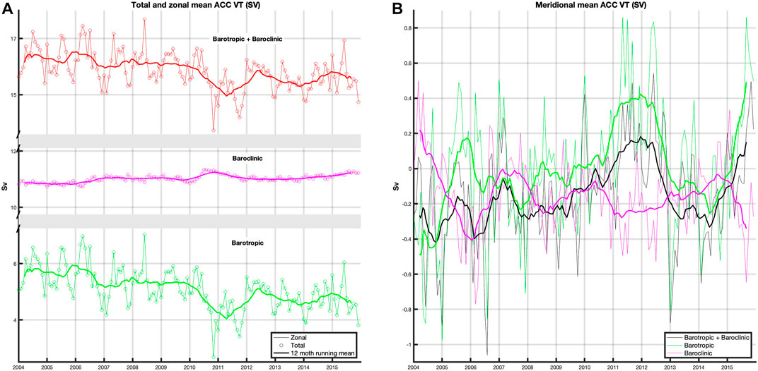
FIGURE 6. Volume transport in the ACC region per 1° gridcell. (A) Zonal (thin curves) and total (circles) VT. Barotropic transport is shown in green, baroclinic transport in magenta, and their sum (barotropic+baroclinic) in red. (B) Mean meridional (thin curves) VT barotropic transport is shown in green, baroclinic transport in magenta, and their sum (barotropic+baroclinic) in black. Thick curves represent a 12-month running mean. Units are Sv.

From Figure 6A, it is possible to obtain an estimation of the zonal VT at a given meridional section of the ACC by multiplying the zonal value at a certain time by the number of grid points of the corresponding section. This approach enables us to estimate the mean zonal VT for any section at a given longitude. Applying this method to the ACC region, we estimate that the mean zonal VT along a meridian is 190.3 ± 0.1 Sv, given that the average number of grid points in the ACC region per meridional section is 12 and the mean total VT per 1° grid cell is 15.9 ± 0.1 Sv.

In the ACC region, the zonal component is the primary contributor to the total VT, as seen in Figure 6A. The baroclinic component is responsible for around 70% of the total VT, while the remaining 30% is due to the barotropic component, which exhibits notable variability over time. The total VT displays a linear trend of −0.007 ± 0.002 Sv/month, an annual signal with an amplitude of 0.42 ± 0.11 Sv peaking in late May, and a biannual signal with an amplitude of 0.12 ± 0.11 Sv peaking in the fifth month of the 24-month period. Comparing our updated estimates to those of the work of Vigo et al. (2018), we observe that despite integrating up to near full depth, our estimates indicate a smaller total VT. This is expected as the results in the study by Vigo et al. (2018) were likely overestimated, as suggested by the comparison with literature in the DP.

It is important to note that our study reports a significant reversal in the contribution of the barotropic and baroclinic components compared to the previous study by Vigo et al. (2018). Specifically, in our study, the barotropic component accounts for only 30% of the total transport, whereas in the earlier study, it was reported to contribute 75%. This difference is due to the use of different reference levels to define the barotropic and baroclinic components. In our study, we consider the VT at 4,900 m depth as the reference level, which is expected to result in a weaker barotropic transport due to smaller geostrophic velocities compared to the reference layer at 1,975 m depth used by Vigo et al. (2018). Figure 6B displays the meridional VT of the ACC region and its barotropic and baroclinic components, with mean values not significantly different from zero in all cases.

4.2.3 Spatial variability of volume transport

To investigate the spatial variability of VT in the Southern Ocean and the ACC, we present a longitudinal series of VT, as well as its zonal and meridional components, in Figure 7. The zonal and meridional longitudinal series are obtained by first taking the time average of each grid point and then integrating latitudinally over the entire Southern Ocean region (65°S–20°S, Figure 7A) and the ACC region (Figure 7B). The total VT longitudinal series is obtained by taking the norm of the zonal and meridional longitudinal series. Our analysis reveals that the mean total VT for the Southern Ocean and the ACC region is 208.4 ± 3.7 Sv and 210.4 ± 3.4 Sv, respectively (Figure 7). It is noteworthy that the mean latitude-sum total VT transport for the ACC region is greater than that for the Southern Ocean region, even though the latter includes the former. This is because the zonal VT longitudinal series has a higher mean value of 198.5 ± 2.9 Sv over the ACC region, compared to the mean value over the entire Southern Ocean region of 178.5 ± 2.58 Sv. The mean value is greater in the ACC region due to the main eastward component of the ACC, while in the Southern Ocean region, outside the ACC, there are regions where the zonal VT has a westward direction (see vector directions in Figure 5A outside the ACC region).

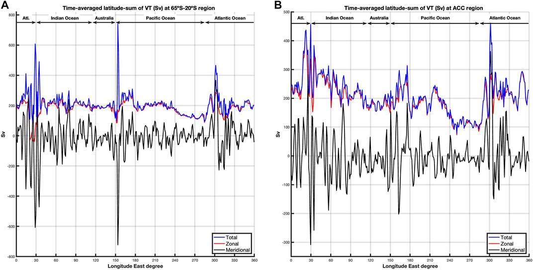
FIGURE 7. Longitudinal series of total (blue curve), zonal (red curve), and meridional (black curve) VT. These longitudinal series are obtained by averaging the data over time and integrating it latitudinally at each longitude across the specified regions. (A) Whole region (65^◦S to 20^◦S) and (B) ACC region (as outlined in Figure 5B).

The longitudinal series of VT and its zonal and meridional components in both the Southern Ocean and ACC regions show that the zonal components dominate the total VT. The zonal VT also drives the low-frequency variability, while the meridional VT drives the high-frequency variability due to the meandering of currents and eddy structures. The baroclinic VT drives the low-frequency variability in both zonal and meridional components, while the barotropic VT drives the high-frequency variability. Note that Figure 7 does not show either the barotropic or the baroclinic components for clarity purposes.

We identify three prominent maxima in the total VT shown in Figure 7A, which coincide with the major local currents acting as borders for the three ocean basins. The first peak is located around 30°E, corresponding to the Agulhas Current, which approximately separates the Atlantic Ocean from the Indian Ocean. From this point, the total VT remains relatively steady at around 200 Sv until we reach 150°E, where the East Australian Current is located, making the transition from the Indian Ocean to the Pacific Ocean. Here, the total VT stabilizes again at around 200 Sv until we reach the Brazil-Malvinas Current at 300°E. Beyond this point, the Atlantic Ocean extends until 30°E.

The longitudinal structure of the ACC, as shown in Figure 7B, exhibits notable similarities to that of the Southern Ocean region. Nevertheless, the peak linked to the East Australian Current at 150°E appears to be less conspicuous in the ACC. Conversely, a new minimum can be discerned between 120°E and 150°E, corresponding to the choke point near South Australia. The decline in VT between 280°E and 300°E is more accentuated in the ACC, which reflects the minimal VT in this region. Additionally, the decay from west to east in each basin is more prominent in the ACC.

A comparison of our new results with those of the work of Vigo et al. (2018) reveals that the VT has been significantly reduced in both the Southern Ocean and the ACC regions (see Supplementary Figure S2 and tables for estimated VT values up to a depth of 1,975 m). This confirms the argument that previous estimates may have overestimated the VT. In our new estimates, the three peaks of the time-averaged latitude-sum VT are less prominent. Only one of the three local minima in the zonal and total VT, corresponding to the DP (between 280°E and 300°E), appears in our Figure 7A, although less prominently. In Figure 7B, the minimum between 280°E and 300°E is more pronounced, and a minimum between 120°E and 150°E is also evident. Additionally, the decay from west to east in each basin is much smoother in our new estimates than in the previous approach (Vigo et al., 2018), particularly in the Pacific Ocean.

4.3 Drake passage

The DP, located between South America and Antarctica, is a natural strait that causes the ACC to narrow, making it a region of great interest for studying ocean circulation. The transport through this choke point has been extensively studied by various monitoring programs, resulting in multiple estimates of the VT based on in situ measurements. In Figure 8, we present our estimated mean SGC speeds for 2004–2015 for the DP region, represented by mean vectors (black arrows) with background color indicating their norm. The three main fronts of the ACC are highlighted in lilac. Additionally, we superimpose five different paths corresponding to the lines of moorings used to estimate the DP VT in the different in situ data-based studies. We have highlighted those of the work of Cunningham et al. (2003) in black squares, Firing et al. (2011) in green circles, Koenig et al. (2014) in red circles, Chidichimo et al. (2014) in yellow triangles, and Olivé Abelló et al. (2021) in gray diamonds. Since we are using satellite data, which provide full coverage of the region, in this section, we will provide our estimates for the DP VT along the different paths where in situ measurements were taken during several campaigns. Although some studies do not overlap with our study period, comparing and validating our results against previous estimates allows us to reconcile discrepancies across in situ data-based studies in the region. This further enables us to demonstrate how different paths for different campaigns might contribute to the various reported estimates of the VT of the DP. By doing so, we can provide a more comprehensive understanding of the DP VT and its variability over time. It is important to note that our study period covers a full decade, which is longer than most previous studies, and our methodology is based on satellite data, which provides a more complete and accurate picture of the ocean circulation in the region.

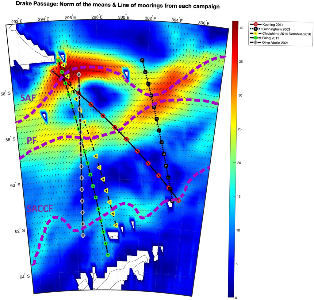
FIGURE 8. Estimated SGC speed (cm/s) for the Drake Passage region, represented by mean vectors (black arrows) with background color indicating their norm. The three main fronts of the ACC (SAF, PF, and SACCF from north to south) are highlighted in lilac. Five different paths corresponding to the line of moorings from different in situ campaigns are highlighted as follows: those by Cunningham et al. (2003) in black squares, Firing et al. (2011) in green circles, Koenig et al. (2014) in red circles, Chidichimo et al. (2014) in yellow triangles, and Olivé Abelló et al. (2021) in gray diamonds.

4.3.1 Drake passage geostrophic velocities

To compare the estimated 3D geostrophic velocities, we present two vertical sections of the zonal velocities for two different longitudes near the DP in Figures 9, 10. These longitudes were chosen to facilitate comparison with the estimates provided by Cunningham et al. (2003) and Olivé Abelló et al. (2021). In Figure 9, we show the mean annual zonal geostrophic velocity along longitude 303.5°E, near the section used by Cunningham et al. (2003), as the colored background for each year from 2004 to 2015. Superimposed on this background are the mean SGC zonal velocities along the same longitude for each year, shown as circled black lines. The units on the left axis correspond to depth (m), and the units on the right axis correspond to speed (cm/s). In this section, only the SAF and PF of the main fronts are visible, and they get closer and apart over time.

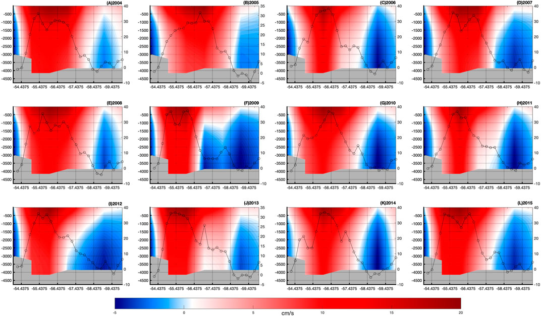
FIGURE 9. Vertical section for the zonal geostrophic velocity (colored background) along the longitude 303.5°E, near the section used by Cunningham et al. (2003), from the surface to 4,900 m depth. Units are cm/s. The SGC zonal velocities are superimposed as black circled lines. Units are cm/s (right axis). Each panel represents the mean for each year for the period 2004–2015, for both the zonal geostrophic velocity and the SGC zonal velocities. The horizontal axis shows latitude, right vertical axis shows depth, and left vertical axis shows the velocity for the SGC zonal velocities.

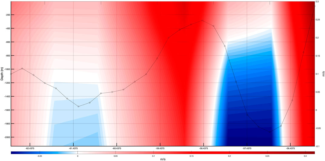
FIGURE 10. Vertical section for the mean 2004–2015 zonal geostrophic velocity (colored background) along the longitude 296.5°E, the same as in the study by Olivé Abelló et al. (2021), from the surface to 2,100 m depth. Units are m/s. The mean 2004–2015 SGC zonal velocity is superimposed as a black circled line. Units are m/s. Horizontal axis shows latitude, right vertical axis shows depth, and left vertical axis shows the velocity for the SGC zonal velocity (m/s).

Figure 9 can be compared with figure 3B from the study by Cunningham et al. (2003), which shows the different mean zonal geostrophic velocities for multiple years between 1993 and 2000 based on in situ measurements. Despite the difference in time period and spatial resolution, we obtain similar results.

In figure 3B from the study by Cunningham et al. (2003), distinct patterns in the zonal geostrophic velocity structure can be observed depending on the proximity of the two fronts. One structure is similar to the one from the year 1999 in figure 3B from the study by Cunningham et al. (2003), where the two fronts are closer near 56.5°S and appear as a single strong eastward component that propagates from the surface to 2,000 m deep. In our results, a similar pattern is shown in Figures 9G,K, which corresponds to the years 2010 and 2014, respectively. These figures also show a single, strong eastward component near the 56.5°S latitude, both for the zonal geostrophic velocity structure (background color) and for the SGC zonal velocities (black circled line).

The other type of structure resembles that of the year 1997 in figure 3B from the study by Cunningham et al. (2003), where two strong eastward components near 55.5°S and 57.5°S, from the surface to 2,000 m depth, are depicted. Our results also exhibit this type of structure in Figures 9D,L for the years 2007 and 2015, respectively. In these cases, the two local maxima near 55.5°S and 57.5°S are distinguishable in the SGC zonal velocities obtained with 0.25° resolution. However, only a single wide, strong eastward component centered at 56.5°S and extending from the surface to 2,000 m depth is visible in the zonal geostrophic velocity profile due to the limited 1° resolution for the 3D geostrophic estimates. The local maxima near 55.5°S and 57.5°S correspond to the SAF and PF fronts, respectively (see Figure 8).

The positions of these fronts, as studied by Sokolov and Rintoul (2009a), can shift over time. The structure with one maximum near 56.5°S corresponds to a time when the SAF and PF fronts are so close that they cannot be distinguished with a 1° resolution. This relationship between front positions and SGC velocities is further illustrated in Figure 11, which shows the mean annual SGC velocities for the years 2007, 2010, 2014, and 2015 in the DP region. The section at longitude 303.5°E is denoted by black circles. In 2010 and 2014, the SAF and PF are closely spaced, forming a large maxima zone around 56.5°S. In contrast, in 2007 and 2015, the SAF and PF are more separated, creating two maxima zones, one near 55.5°S and the other near 57.5°S.

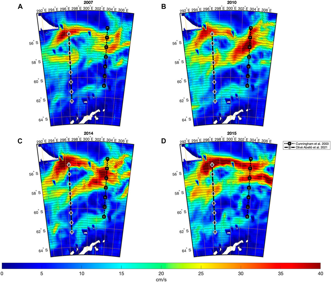
FIGURE 11. Estimated SGC speed for the Drake Passage region, represented by mean vectors (black arrows) with background color indicating their norm (units: cm/s). Annual mean for the years (A) 2007, (B) 2010, (C) 2014, and (D) 2015 is given. Section [60.5°S, 54.5°S] x [303.5°E] [the closest meridional section to the one used in the study by Cunningham et al. (2003)] is highlighted as black squares, and section [62.5°S, 55.5°S] x [296.5°E] [same as in the study by Olivé Abelló et al. (2021)] is highlighted as gray diamonds.

Figure 10 presents the mean 2004–2015 zonal geostrophic velocity (background color) and the mean 2004–2015 SGC zonal velocity (circled black lines) at longitude 296.5°E, which is the same meridional section as in the study by Olivé Abelló et al. (2021). Annual mean profiles are not included due to their high similarity. Figure 11 shows the mean annual SGC velocities for the years 2007, 2010, 2014, and 2015 in the DP region, with the section at longitude 296.5°E denoted by gray diamonds. For all the years shown, there are always three local maxima zones at the same latitudes (63°S, 59°S, and 56°S) for the 296.5°E section (gray diamonds). Comparing Figure 10 in this study with the bottom left panel of figure 7 in the study by Olivé Abelló et al. (2021), it becomes evident that the findings from both studies are in excellent agreement. Three prominent eastward components are distinctly identified, located at approximately 63°S, 59°S, and 56°S, for both the zonal geostrophic velocity and SGC zonal velocity, which correspond to the three primary fronts SACCF, PF, and SAF. The numerical values obtained from both approaches are highly similar, although our results are slightly less intense.

4.3.2 Drake passage volume transport

To validate our VT results, the total VT through the DP was computed and compared with the results from previous studies, which were mostly based on in situ data. These studies include those by Cunningham et al. (2003), Firing et al. (2011), Koenig et al. (2014), Chidichimo et al. (2014), Donohue et al. (2016), and Olivé Abelló et al. (2021). To calculate the corresponding VT for each of these studies, the grid points that follow the mooring lines were defined (Figure 8), and each VT estimation at the DP was obtained by adding the VT vectors of such grid points. It is important to note that the lines of moorings used do not follow a meridian as they have a certain degree of inclination; thus, what is being reported is the perpendicular transport through each line.

Table 2 presents the comparison of our VT estimates with previously reported values from different studies in the DP region. Our findings for depths other than the bottom are consistent with those of other investigations. Specifically, our study results are in good agreement with those reported by Firing et al. (2011), Koenig et al. (2014), Chidichimo et al. (2014), and Donohue et al. (2016). However, our full-depth VT estimate following the path from the work of Olivé Abelló et al. (2021) aligns more closely with their 2,000 m depth estimate. In terms of the full-depth VT reported in the literature, our estimates generally fall within the reported values, albeit towards the higher end of the range, taking into account the error range. For instance, Koenig et al. (2014) reported a full-depth VT range of [117, 220] Sv, which is consistent with our result. However, it is noteworthy that our results exhibit a larger standard deviation than previous studies based on in situ data. It is important to note that in order to estimate the VT for the full depth, both our estimates and in situ estimates rely on interpolated data. Specifically, there are no ARGO data available from 2,000 m to the bottom, which makes our full-depth VT estimates less reliable. Nonetheless, we find that our results are in good agreement with previous studies for the total VT depths of 1,000 m, 2,000 m, and 3,000 m, which should be more accurate. These findings support our claim that our estimated total VT is robust for the DP area, where the mean depth is 3,500 m.

TABLE 2. Comparison of total transport through the Drake Passage between studies by several authors and our study. Units are Sv. For the results of this study, we always follow the different sections of each study and give the perpendicular transport for each section (mean ± std).

An advantage of this methodology based on satellite data is that we can retrieve the VT for the entire period of study and analyze its temporal variation. Figure 12 displays the time series for the various VT components through the DP at longitude 303.5°E within the ACC region. The thin lines represent all the raw time series, while the thick line shows a 12-month running mean.

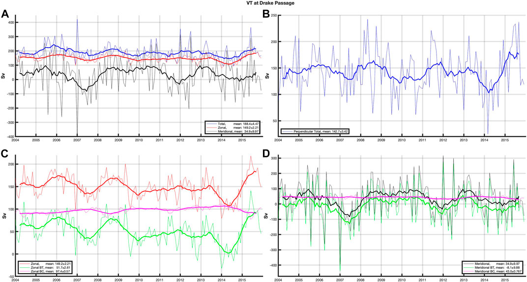
FIGURE 12. VT at the Drake Passage, following the longitude section [60.5°S, 54.5°S] x [303.5°E] near the section from the study by Cunningham et al. (2003): (A) Zonal (red), meridional (black), and total (blue) VT. (B) Total perpendicular transport (blue) across the section used in the study by Cunningham et al. (2003). (C) Zonal (red), zonal barotropic (green), and zonal baroclinic (magenta). (D) Meridional (black), meridional barotropic (green), and meridional baroclinic (magenta). For all figures, thick curves are 12-month running means.

Figure 12A illustrates the temporal variation of the total (blue) VT through the DP and its zonal (red) and meridional (black) components. The total VT shows relatively stable behavior throughout the study period, with a mean signal of 188.4 ± 4.5 Sv. The zonal component is the primary contributor to the signal and shows a stable behavior as well, with a mean signal of 149.2 ± 2.2 Sv and a high correlation with the total VT at 0.5 (p-value < 0.001). However, the meridional component displays more variability, with a mean signal of 34.9 ± 9.9 Sv, caused by the meandering and eddy structures formed periodically in the region. Neither the total VT in the DP (blue line in Figure 12A) nor the total perpendicular VT in the DP (blue line in Figure 12B) displays significant annual, semiannual, biannual, or linear trends.

Figure 12C illustrates the decomposition of the zonal VT (red line) from Figure 12A into its barotropic (green) and baroclinic (magenta) components. The barotropic component, with a mean signal of 51.7 ± 2.6 Sv, represents 35% of the total zonal transport, while the baroclinic component, with a mean signal of 97.4 ± 0.6 Sv, represents 65%. The variability of the zonal transport is predominantly driven by its barotropic component, with a high correlation of 0.98 (p-value < 0.001) between the total zonal VT and its barotropic component.

The meridional component (blue) from Figure 12A is shown in Figure 12D, along with its barotropic (green) and baroclinic (magenta) components. Similar to the zonal component, the variability in the meridional transport is also largely driven by its barotropic component, as evidenced by the high correlation of 0.99 (p-value < 0.001) between the total meridional VT and its barotropic component.

5 Conclusion

In this study, we present a geodetic approach to investigate the near full-depth 3D geostrophy and VT in the SO spanning from 20°S to 65°S by utilizing space data from Altimetry and Gravity satellite missions, as well as T and S profiles. Our approach expands upon the work of Vigo et al. (2018), who presented a similar methodology based on satellite data (SSH from altimetry and an independent geoid based mainly on GOCE data) for the Southern Ocean up to a depth of 1,975 m, covering the period 2004–2014 with monthly resolution and 1° spatial resolution. While the approach by Vigo et al. (2018) proved the advancement in precision and resolution over previous approaches based on a GRACE geoid (Mulet et al., 2012; Kosempa and Chambers, 2014; Carter et al., 2008), validation with in situ data revealed an overestimation of the currents and associated VT. In this study, we have revisited this issue and updated all the datasets involved in the analysis (geoid, MSS, SSH, and T and S profiles) to provide a new estimate of the 3D geostrophy and VT up to near full depth (4,900 m), expanding the study period to 2004–2015. Although the values obtained in this study are lower than those reported in the previous approach, the new findings provide higher detail in the currents and are closer to observations reported in previous studies (Cunningham et al., 2003; Beal et al., 2015; Sloyan et al., 2016; Artana et al., 2018).

Upon focusing on the ACC, we have found that the mean VT for each 1° cell with the new data stands at 15.9 ± 0.1 Sv, which is almost 50% lower than that reported by Vigo et al. (2018). The baroclinic and barotropic components of the VT have also been estimated, revealing that 70% of the total transport is baroclinic. It should be noted, however, that these results are not directly comparable with previous estimates, as the reference depth for barotropic transport is now defined using the bottom, whereas in the study by Vigo et al. (2018), the reference was 1,975 m.

In terms of variability, the ACC mean VT exhibits an annual signal with an amplitude of 0.42 ± 0.11 Sv that peaks in May, a linear trend of −0.007 ± 0.002 Sv per month, and a biannual signal with an amplitude of 0.12 ± 0.11 Sv that peaks in the 5th month of the 24-month period. The annual and biannual signals have been confirmed to be of barotropic origin, as well as the interannual variability, while the baroclinic signal remains steady at around 11 Sv for the entire period.

Regarding the DP VT, our geodetic approach has yielded estimates that are highly consistent with previous literature values, with good agreement observed across multiple campaigns and paths defined by the lines of moorings. Notably, the perpendicular transport to these lines closely matches reported values, which vary between 136 and 173 Sv depending on the location of the lines. Our approach, based on satellite data and providing global coverage, has, thus, succeeded in reconciling the discrepancies reported in earlier literature. To provide a specific value for the DP VT, we propose using the zonal transport along 303.5°E within the ACC region, which is the closest meridional section to the classical section by Cunningham et al. (2003). Our analysis yields an estimated mean VT of 149.2 ± 2.2 Sv using this approach.

In conclusion, the proposed methodology has demonstrated its utility in providing global and regional estimates of ocean GC, which are integral to our understanding of ocean circulation. By updating the satellite altimetry data for sea surface height, satellite-derived geoid, and temperature and salinity profiles, we have improved our estimates of the Southern Ocean 3D GC and VT, with good agreement observed between our results and previous approaches based on in situ data. Notably, our approach has reconciled varying estimates in the literature by considering the exact location of measurements. Overall, our study contributes to the understanding of the Southern Ocean’s 3D geostrophic currents, provides robust VT estimates, and validates the results through careful comparison with in situ measurements.

Looking ahead, we anticipate that future satellite missions and innovative concepts for satellite-based gravity missions will continue to improve our knowledge of sea surface height and the geoid, leading to even higher resolution and precision in our estimations of ocean geostrophic currents from satellite data. These advancements in our understanding of ocean circulation will be critical for furthering our knowledge of Earth’s climate system, particularly in light of ongoing changes in the ocean’s role in regulating the planet’s heat budget and carbon cycle. By refining our ability to measure and model the ocean’s dynamic processes, we can improve our ability to predict and mitigate the impacts of climate change on our planet and society.

Data availability statement

Publicly available datasets were analyzed in this study. These data can be found at: http://www.esa-sealevel-cci.org, https://www.metoffice.gov.uk/hadobs/en4/.

Author contributions

JV-A and MV conceived and designed the study. MV and DG-G processed the data and obtained the 3D geostrophy and VT. JV-A, MV, and FZ analyzed the data. All authors contributed to the article and approved the submitted version.

Funding

This research is support by grant PID2021-122142OB-I00 funded by MCIN/AEI/10.13039/501100011033, grant PROMETEO/2021/030 funded by Generalitat Valenciana, and grant GVA-THINKINAZUL/2021/035 funded by Generalitat Valenciana and “European Union NextGenerationEU/PRTR”.

Acknowledgments

The authors acknowledge the support of all data providers: ESA in the frame of the CCI Sea Level Project for Altimetry data; DTU SPACE from the Danish National Space Center for MDT and MSS products; and the Met Office Hadley Center for EN4.1.1 data product.

Conflict of interest

The authors declare that the research was conducted in the absence of any commercial or financial relationships that could be construed as a potential conflict of interest.

Publisher’s note

All claims expressed in this article are solely those of the authors and do not necessarily represent those of their affiliated organizations, or those of the publisher, the editors, and the reviewers. Any product that may be evaluated in this article, or claim that may be made by its manufacturer, is not guaranteed or endorsed by the publisher.

Supplementary material

The Supplementary Material for this article can be found online at: https://www.frontiersin.org/articles/10.3389/feart.2023.1110138/full#supplementary-material

SUPPLEMENTARY FIGURE S1 | Same as Figure 5 but VT integrated only up to 1,975 m depth.

SUPPLEMENTARY FIGURE S2 | Same as Figure 7 but VT integrated only up to 1,975 m depth.

References

Andersen, O., Knudsen, P., and Stenseng, L. (2018). “A new DTU18MSS Mean Sea Surface – improvement from SAR altimetry,” in Abstract from 25 years of progress in radar altimetry symposium, Portugal, September 2018.
Artana, C., Ferrari, R., Koenig, Z., Sennéchael, N., Saraceno, M., Piola, A. R., et al. (2018). Malvinas current volume transport at 41°S: A 24 yearlong time series consistent with mooring data from 3 decades and satellite altimetry. J. Geophys. Res. Oceans 123 (1), 378–398. doi:10.1002/2017JC013600
Beal, L., Elipot, S., Houk, A., and Leber, G. (2015). Capturing the transport variability of a western boundary jet: Results from the Agulhas current time-series experiment (ACT). J. Phys. Oceanogr. 45 (5), 1302–1324. doi:10.1175/JPO-D-14-0119.1
Carter, L., Mccave, I. N., and Williams, M. J. M. (2008). Chapter 4 circulation and water masses of the Southern Ocean: A review. Amsterdam, Netherlands: Elsevier, 1571–9197. doi:10.1016/s1571-9197(08)00004-9
Chidichimo, M. P., Donohue, K. A., Watts, D. R., and Tracey, K. L. (2014). Baroclinic transport time series of the antarctic circumpolar current measured in Drake passage. J. Phys. Oceanogr. 44 (7), 1829–1853. doi:10.1175/jpo-d-13-071.1
Cunningham, S. A., Alderson, S. G., King, B. A., and Brandon, M. A. (2003). Transport and variability of the antarctic circumpolar current in Drake passage. J. Geophys. Res. 108, 8084. C5 ISSN 0148-0227. doi:10.1029/2001jc001147
Donohue, K. A., Tracey, K. L., Watts, D. R., Chidichimo, M. P., and Chereskin, T. K. (2016). Mean antarctic circumpolar current transport measured in Drake passage. Geophys. Res. Lett. 43 (22), 0094–8276. doi:10.1002/2016gl070319
Firing, Y. L., Chereskin, T. K., and Mazloff, M. R. (2011). Vertical structure and transport of the antarctic circumpolar current in Drake passage from direct velocity observations. J. Geophys. Res. 116, C08015. doi:10.1029/2011JC006999
Fofonoff, N. P. (1962). “Dynamics of ocean currents,” in Wiley-interscience. 1 (Hoboken, NJ, United States: The Sea), 323–395. Physical Oceanography.
Good, S. A., Martin, M. J., and Rayner, N. A. (2013). EN4: Quality controlled ocean temperature and salinity profiles and monthly objective analyses with uncertainty estimates. J. Geophys. Res. Oceans, Dec. 118 (12), 6704–6716. doi:10.1002/2013JC009067
Knudsen, P., Andersen, O., Maximenko, N., and Hafner, J. (2019). “A new combined mean dynamic topography model -DTUUH19MDT,” in Anonymous Living Planet Symposium, Milan, Italy, May 2019.
Koenig, Z. E., Provost, C., Ferrari, R., Sennéchael, N., and Rio, M. (2014). Volume transport of the Antarctic Circumpolar Current: Production and validation of a 20 year long time series obtained from in situ and satellite observations. J. Geophys. Res. Oceans 119 (8), 5407–5433. doi:10.1002/2014jc009966
Kosempa, M., and Chambers, D. P. (2014). Southern Ocean velocity and geostrophic transport fields estimated by combining Jason altimetry and Argo data. J. Geophys. Res. Oceans 119 (8), 4761–4776. doi:10.1002/2014JC009853
Mcdougall, T. J., and Barker, P. M. (2011). Getting started with TEOS-10 and the Gibbs seawater (GSW) oceanographic 423 Toolbox. Scor/Iapso WG 532, 1–28. version 3.0 (R2010a). ISBN 978-0-646-55621-5.
Mulet, S., Rio, M., Mignot, A., Guinehut, S., and Morrow, R. (2012). A new estimate of the global 3D geostrophic ocean circulation based on satellite data and in-situ measurements. Deep-Sea Res. Part II, Top. Stud. Oceanogr. 77-80, 70–81. doi:10.1016/j.dsr2.2012.04.012
Olivé Abelló, A., Pelegrí, J. L., Machín, F. J., and Vallès-Casanova, I. (2021). The transfer of antarctic circumpolar waters to the western south Atlantic Ocean. J. Geophys. Res. Oceans 126 (7), 2169–9275. doi:10.1029/2020jc017025
Orsi, A. H., Whitworth, T., and Nowlin, W. D. (1995). On the meridional extent and fronts of the Antarctic Circumpolar Current. Deep Sea Res. Part I Oceanogr. Res. Pap. 42 (5), 641–673. doi:10.1016/0967-0637(95)00021-w
Sloyan, B. M., Ridgway, K. R., and Cowley, R. (2016). The East Australian current and property transport at 27°S from 2012 to 2013. J. Phys. Oceanogr. Mar 46 (3), 993–1008. doi:10.1175/JPO-D-15-0052.1
Sokolov, S., and Rintoul, S. R. (2009a). Circumpolar structure and distribution of the antarctic circumpolar current fronts: 1. Mean circumpolar paths. J. Geophys. Res. 114, C11018. doi:10.1029/2008jc005108
Sokolov, S., and Rintoul, S. R. (2009b). Circumpolar structure and distribution of the antarctic circumpolar current fronts: 1. Mean circumpolar paths. J. Geophys. Res. 114 (C11), C11018. doi:10.1029/2008JC005108
Tarakanov, R. Y. (2021). “Multi-jet structure of the antarctic circumpolar current,” in Antarctic peninsula region of the Southern Ocean. Editors E. G. Morozov, M. V. Flint, and V. A. Spiridonov (Cham: Springer), 6. Advances in Polar Ecology. doi:10.1007/978-3-030-78927-5_2
Vigo, M. I., García-García, D., Sempere, M., and Chao, B. F. (2018). 3D geostrophy and volume transport in the Southern Ocean. Remote Sens. 10, 715. doi:10.3390/rs10050715
Whitworht, T. (1983). Monitoring the transport of the antarctic circumpolar current at Drake passage. J. Phys. Oceanogr. doi:10.1175/1520-0485
Whitworth, T., and Peretson, R. G. (1985). Volume transport of the antarctic circumpolar current from bottom pressure measurements. J. Phys. Oceanogr. 15, 810–816. doi:10.1175/1520-0485(1985)015<0810:vtotac>2.0.co;2
Keywords: 3D geostrophy, volume transport, Southern Ocean, Antarctic Circumpolar Current, satellite altimetry, satellite gravity
Citation: Vargas-Alemañy JA, Vigo MI, García-García D and Zid F (2023) Updated geostrophic circulation and volume transport from satellite data in the Southern Ocean. Front. Earth Sci. 11:1110138. doi: 10.3389/feart.2023.1110138
Received: 28 November 2022; Accepted: 30 June 2023;
Published: 21 July 2023.
Edited by:
Xiaopeng Li, National Geodetic Survey, United StatesReviewed by:
Milena Menna, National Institute of Oceanography and Experimental Geophysics (Italy), ItalyXiaoyun Wan, China University of Geosciences, China
Andreas Reul, University of Malaga, Spain
Copyright © 2023 Vargas-Alemañy, Vigo, García-García and Zid. This is an open-access article distributed under the terms of the Creative Commons Attribution License (CC BY). The use, distribution or reproduction in other forums is permitted, provided the original author(s) and the copyright owner(s) are credited and that the original publication in this journal is cited, in accordance with accepted academic practice. No use, distribution or reproduction is permitted which does not comply with these terms.
*Correspondence: M. Isabel Vigo, vigo@ua.es
†ORCID: Juan A. Vargas-Alemañy, orcid.org/0000-0002-4958-5607; M. Isabel Vigo, orcid.org/0000-0002-6102-946X; David García-García, orcid.org/0000-0002-7273-9037