Particle tracking as a vulnerability assessment tool for drinking water production

1 Introduction

Drinking water contamination is a major matter of concern for worldwide public health, with worldwide economic and social effects (Daud et al., 2017; Sharma and Bhattacharya, 2017; Gwimbi et al., 2019; Turner et al., 2021). This emphasizes the need for decision-support modeling tools that could provide 1) reliable predictions of the risk associated with water contamination in prospective scenarios and 2) optimized production settings to mitigate the impact of reported contamination. To this end, models may be of great interest provided a series of conditions are satisfied (Doherty, 2015; Hermans, 2017; Doherty and Moore, 2020). First, that models should properly account for the processes governing the outputs of interest. Second, that an appropriate and reliable observational dataset constrains the parameters of importance. Third, that the model is “practical”, which implies reasonable computation time and effective tools to automatize time consuming operations (Bakker et al., 2016; White et al., 2020a). Such conditions may not be easy to fulfill, in particular when dealing with the complex process of contaminant transport in heterogeneous aquifers.

In such a context, a thorough analysis of the simplicity-complexity trade-off becomes a critical step for which guidelines are now available (Hrachowitz et al., 2014; Guthke, 2017; Schwartz et al., 2017; Hugman and Doherty, 2022). In practice, appropriate choices have to be made on 1) the parameterization of hydraulic and transport properties and 2) the simulated physio-chemical processes driving the propagation of contaminant. For the parameterization of hydraulic properties, the options range from homogeneous equivalent hydraulic conductivity zones to heterogeneous fields with discrete features (de Marsily et al., 2005; Carniato et al., 2015; Pool et al., 2015). For the selection of processes governing transport, the options range from simplified models that rely on assumptions such as steady-state and dominant processes (e.g., advection), to complex, advection-dispersion reactive transport models to provide a detailed description of the physics of the problem (Anderson et al., 2015). Several studies highlighted that the best balance in terms of robustness, efficiency and reliability may be achieved with relatively simple “surrogate” models based on simplified representations of the physics (Razavi et al., 2012; Asher et al., 2015; Burrows and Doherty, 2015). Surrogate transport models present fast run times allowing for thousands of model executions of transport calculations, which are necessary for history matching of highly parameterized models. The interest of including a diverse observational data types has been highlighted by Hunt et al. (2006) and concentration in particular has been recently discussed by Schilling et al. (2019) and Knowling et al. (2020). Furthermore, fast run time allows the use of more robust but demanding algorithms for uncertainty quantification (Rajabi et al., 2018).

During the last decades, parameter estimation and uncertainty quantification algorithms have been made available with an ever growing variety of approaches (Doherty, 2016; White et al., 2020b). Their use is now facilitated by Python interfaces (White et al., 2016). More recently, studies provided repeatable script-based workflows which greatly facilitate the replication of the presented approaches (White et al., 2020a; Fienen et al., 2022). Though facilitated, the interfacing of parameter estimation and uncertainty quantification algorithms with complex models remains difficult for transport models, which are characterized by long computation times and numerical instabilities.

Focusing on the widely reported risk of contaminant transfer from contaminated rivers to groundwater production units, we present a framework based on particle tracking as a fast and effective surrogate model for contaminant transport. The approach, initially presented by (Cousquer et al., 2018), is made available in a newly developed Python module, TrackTools which will facilitate its replication. The module provides particle seeding capabilities and post-processing options that are valuable for analyzing drinking water vulnerability of production wells or drains to pre-defined sources of contamination. The script facilitates exploratory parametric analysis, which can be useful to investigate the system response to different configurations. The interfacing with the PEST + + suite (White et al., 2020b) is detailed on a real-world case study which paves the way for history matching, hypothesis testing, and optimization of decision variables, which are essential to support decision related to the definition of wellhead protection area and the optimization of production settings.

The theoretical background and numerical tools related to the developed Python module are described in Section 2. A simple synthetic model is presented in Section 3 and a parametric study is conducted to investigate the driving factors of mixing ratios computed with this approach. In Section 4, the interest of the method is illustrated on a drinking water production site with a fully script-based approach from model setup to pumping optimization through parameter estimation.

2 Methodology

A common practice in vulnerability analysis is to investigate the origin of water withdrawn at a groundwater sink (well or drain) originating from one, or a series of potential or effective contaminant sources. This can be conducted from the analysis of the flow contributions of each source to the discharge rate of the sink. The methodology described hereafter is an extension of the approach described by Cousquer et al. (2018) initially designed for a single river reach. The method may now be applicable to multiple weak or strong source boundary conditions (e.g., fixed head, river, general head boundary condition).

Consider a groundwater flow model with a groundwater sink (well or drain) subject to a potential are effective contamination originating from one of the model boundary conditions. A set of N starting points is seeded around the model cells where the sink condition is applied. Given the flow field, the origin of flow to the sink can be described by backward particle tracking.

The sink discharge rate Q can then be decomposed as follows: $Q={\sum }_{i=1}^N{q}_i$, where q_i is the contribution of the i-th particle to the discharge rate at the sink. This can be rewritten considering particle velocities, v_i: $Q={\sum }_{i=1}^N{v}_i\cdot S_i$ where S_i is the area of the surface crossed by q_i. When particles are evenly distributed around the model cell, it can be assumed that $S_i=\frac{S}{N}$ for all i.

Assume that from the N particles seeded around the sink, n_j originate from the j − th boundary condition, subject to contamination. The contribution of this boundary condition to the sink contamination can be written as follows:

where β_k is the mixing ratio in the source model cell where the k-th particle ends. β_k = 1 for “strong” sources and 0 ≤ β_k ≤ 1 for “weak sources” where a mixing occurs (Pollock, 2016). In the latter case, β_k can be quantified from the cell water budget at the endpoint cell (Cousquer et al., 2018). This allows the method to account for mixing in the source aquifer cell, where the boundary condition (typically a river) is applied.

The approach is now integrated in the TrackTools Python module. Our approach relies on the USGS MODFLOW6 (Langevin et al., 2017) and MODPATH7 (Pollock, 2016) programs to simulate fluid flow and transport processes, respectively. We rely on the FloPy module (Bakker et al., 2016) for the processing of model input and output files.

Pre-processing capabilities of the TrackTools module are provided in the ParticleGenerator class, which can handle:

• Particle seeding around groundwater sinks, which can be described by a Python geometry or ESRI^TM shapefile,

• Adding, removing and merging particles into groups for FloPy and MODPATH7.

After the simulation of flow with MODFLOW and particle tracking with MODPATH, the TrackingAnalyzer class of TrackTools can be used to process particle pathline data and derive the values of mixing ratios at each groundwater sink. The MODFLOW cell-by-cell water budget file is also required to derive the source cell mixing ratio β_k. Results can be provided in the form of a data frame and plotting options are proposed for the description of the origin of groundwater withdrawn in the series of sinks where particles were seeded.

3 Synthetic case

3.1 Model description

In order to illustrate the presented Python module, a synthetic 2D case is considered with a production well in an unconfined aquifer in interaction with a stream. The domain (3,750 × 5,000 m) is discretized with a 2D regular mesh (25 × 25 m cells) with a local refinement around the stream and the well (6.5 × 6.5 m cells). A Cauchy-type boundary condition is applied to the upper limit of the model domain with a stage of 40 m and conductance of 10^–3 m² s⁻¹, while a Dirichlet-type condition is prescribed to the lower boundary with a stage of 20 m. They are simulated with the General Head Boundary (GHB) and Fixed Head (FH) MODFLOW packages, respectively. The left and right domain boundaries are considered as impermeable. The stream is simulated with a head-dependent flux (Cauchy-type) boundary condition with the dedicated MODFLOW river package (RIV), with a head ranging from 35 m to 25 m from the upper to the lower boundary condition. The stream conductance is set to 10^–3 m² s⁻¹. Steady-state flow conditions are considered and the transmissivity is assumed to be independent of water level fluctuations, which corresponds to the Boussinesq assumption. The well is considered as fully penetrating and is located at position (x, y) = (1212, 1363).

We consider both homogeneous and heterogeneous hydraulic conductivity fields, the heterogeneous cases being generated with an isotropic exponential variogram for log 10(k) defined by a sill of one and a nugget of 0.1 for two different ranges of 200 and 500 m as presented in Figure 1. These fields are generated using the geostatistical python package GSTools (Müller et al., 2021). During the following simulations, the mean hydraulic conductivity value will evolve in heterogeneity patterns (Figures 1B,C).

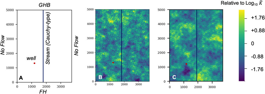
FIGURE 1. (A) Synthetic case model structure and boundary conditions with a General Head Boundary Condition (GHB) of 40 m to the upper boundary and a Fixed Head (FH) of 20 m to the lower boundary. No flow is imposed at the left and right domain boundaries. The stream is simulated with a head-dependent flux (Cauchy-type) boundary condition and the well position is represented with a red dot. The hydraulic conductivity field patterns correspond to an exponential viariogram with a sill of 1, a nugget of 0.1 and a range of (B) 200 m and (C) 500 m.

3.2 Parametric study

The synthetic case previously described is used to illustrate the behavior of the mixing ratio α depending on key parameters such as the hydraulic conductivity K and pumping discharge Q. β from Eq. (1) is quantified from the river cell water budget and can vary from 0 to 1. Figure 2 shows the distribution of α for parameters K and Q ranging from 10^–5 to 10^–3 m s⁻¹ and from 0 to 200 m³ h⁻¹, respectively, considering a homogeneous distribution of K. Boundary conditions remain the same throughout this parametric study. We also present in Figure 3 three examples of the spatial distribution of the hydraulic head H with K set to (A) 10^–5, (B) 10^–4 and (C) 10^–3 m s⁻¹ and the same configuration but with a pumping discharge of 90 m³ h⁻¹ for D, E and F. These values have been chosen as representative of the three main tendencies that are observed for α: 1) the yellow region in which example D is located corresponding to the highest values of α, 2) the dark blue region in which example E is located corresponding to the lowest values of α and, 3) the green region in which example F is located corresponding to intermediate values of α. This shows that increasing K for a given value of Q results in decreasing (from D to E) and then increasing (from E to F) α, except for very small values of Q for which α directly increases (from E to F). These different behaviors are explained by the different sources of water that contribute to the pumped water, which are characterized by the particle paths represented on the hydraulic head distributions in blue. For small values of K (example D), most of the particles comes from the portion of the river that is located right next to the well, implying that the river provides a substantial proportion of water to the pumping well. Increasing K (example E) results in reducing the impact of the pumping on the natural hydraulic head distribution, implying that the top boundary condition contributes to the pumping. When we keep increasing K (example F), we reach configurations that do not depend on the pumping rate (green triangular region on the right side of Figure 2). For these cases, the pumping does not modify the natural hydraulic head distribution and the particle paths are fully driven by the boundary conditions, resulting in particles coming from the top of the river and thus high values of α. For small values of Q and K (black region of the bottom of the figure), the impact of the pumping on the natural hydraulic head distribution is still negligible but the values of K imply that there is no contribution of the river to the pumping (α = 0).

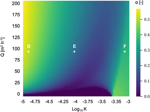
FIGURE 2. Distribution of the mixing ratio α depending on the hydraulic conductivity K and pumping discharge Q.

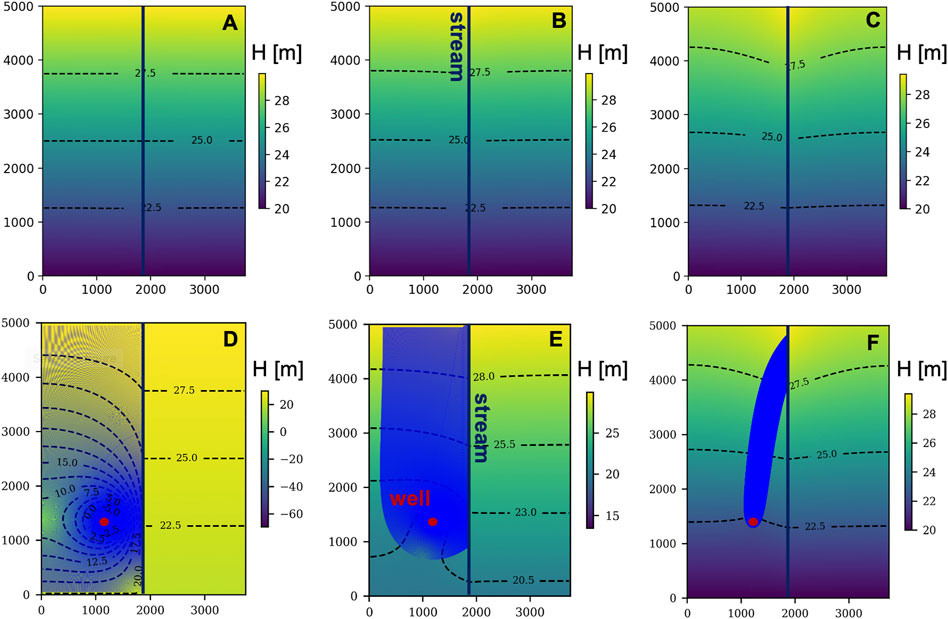
FIGURE 3. The spatial distribution of the hydraulic head H(x, y) for hydraulic conductivity K set to 10^–5 m s⁻¹ (A,D), 10^–4 m s⁻¹ (B,E) and 10^–3 m s⁻¹ (C,F). Cases (A,B,C) are without pumping, while a pumping rate of 90 m³ h⁻¹ is set for cases (D,E,F). The red dot represent the pumping well locations, the vertical bold black line represents the stream and the blue lines in cases (D,E,F) are the path of the particles from the backward particle tracking.

Figure 4 shows the distribution of α when considering the heterogeneous hydraulic conductivity fields provided in Figure 1. The three main tendencies described above for the homogeneous case are also observed for the heterogeneous cases, showing that these behaviors are mostly driven by the boundary, river and pumping conditions. However, small differences are noticeable, in particular for small values of Q and large values of $\bar{K}$, which correspond to configurations with a small impact of the pumping on the natural hydraulic head distribution. For example, the extent of the dark blue region observed at the bottom of Figure 3 is reduced and increased in Figures 4A,B, respectively, showing that the river does not contribute to the pumping for different values of Q and $\bar{K}$. We also observe the presence of yellow areas for large values of $\bar{K}$ in the heterogeneous cases, corresponding to high values of α and thus a strong contribution of the river to the pumping. These different behaviors are due to different flow paths induced by the heterogeneities of the hydraulic conductivity fields. Note that, as mentioned before, the impact of these heterogeneities is reduced when increasing the pumping rate.

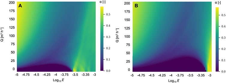
FIGURE 4. Distribution of the mixing ratio α depending on the average hydraulic conductivity $\bar{K}$ and pumping discharge Q for the hydraulic conductivity patterns presented in (A) Figures 1B and (B) Figure 1C.

3.3 Derivative analysis

This synthetic case is also used to set some rules in order to obtain robust derivatives which is essential for parameter estimation and model analysis based on linearization methods. The sufficient number of particles corresponding to this synthetic case is evaluated with the derivative calculation of $\frac{\partial \alpha }{\partial K}$ which constitutes the Jacobian matrix used for model linearization. The use of gradient based methods for parameter estimation (e.g., the Gauss-Marquardt-Levenberg method on which PEST and PEST++ are based (Doherty, 2015; White et al., 2018)) requires that model outputs are differentiable or at least continuous with regard to model parameters (Doherty, 2010). Doherty and Hunt (2010) mentioned that this assumption often does not hold because of poor model performance and the lack of differentiability can be due to, among others reasons, a low number of particles in the MODPATH particle tracking model. In order to avoid this issue, we explore the differentiability of model output regarding particles number. Let the mixing ratio α be the output of interest, the hydraulic conductivity K is the parameter and ΔK is the parameter increment. The sensitivity of α to K is approximated as follows:

The estimate of $\frac{\partial \alpha }{\partial K}$ may be biased when 1) ΔK is too small, due to numerical noise, 2) when ΔK is too large due to model non-linearity, or 3) when the number of particles is not high enough to correctly simulate the mixing ratio. These three points are evaluated by calculating the value of the derivative for several numbers of particles and different values of K_i considering two values of ΔK set to 0.01 × K_i and 0.1 × K_i (Figure 5).

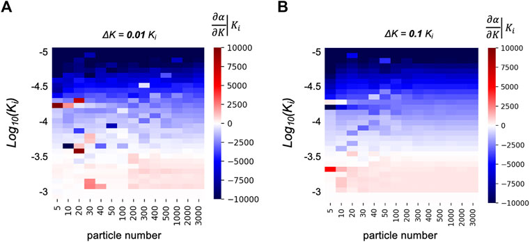
FIGURE 5. Exploration of derivatives quality behaviour regarding the number of particles with the hydraulic conductivity K_i ranging from 10^–5 to 10^–3 m s⁻¹ and the increment ΔK set to (A) 0.01 × K_i and (B) 0.1 × K_i.

For both ΔK = 0.01 × K_i and ΔK = 0.1 × K_i, Figure 5 shows changes in the derivative sign that are visible when the color representing the derivative goes from blue (negative values) to red (positive values) and vice versa. For a given line, these changes depend on the number of particles N_p used in the model, showing wrong estimations of the derivative when N_p is too small (due to wrong estimations of the mixing ratio). This results in instabilities of the derivative along K for small number of particles (N_p < 200−500, columns that are located on the left side of Figure 5). For parameter estimation and inversion purposes, these instabilities could be interpreted as local minima and lead to wrong estimates and optimized values. When N_p is high enough (columns on the right side), the derivative values are stable in the sense that they do not change with the value of N_p. In this case, changes in $\frac{\partial \alpha }{\partial K}$ along K are due to the non-linearity of the model, which needs to be taken into account for parameter estimation and optimization.

Furthermore, comparing Figures 5A,B shows that the choice of the increment of K influences the stability of the derivative. The number of particles that is required to observe stable values of $\frac{\partial \alpha }{\partial K}$ is lower when increasing ΔK.

Although they are expected, these results clearly show that the derivative calculation requires to carefully choose the parameters N_p and ΔK with 1) a sufficient number of particles to correctly simulate the mixing ratios and its derivative, and 2) an increment that is neither too small to avoid that the derivative calculation is tainted by numerical problems, nor too large to take into account the non-linearity of the model. In all cases, increasing the number of particles is a systematic method to improve the definition of the derivative whatever the value of the discretization step of the derivative.

4 Case study

4.1 Model description

The method described above is embedded in a workflow designed for model-based decision making and applied to a complex real world case study. We describe the script-based modeling workflow and interfacing with the PEST + +, which provides an illustration of the interest of the method and facilitates the replication of the approach to other cases. All scripts are available on a GitHub^® repository.

The well field is located in South-West France and is critical to the water supply for the city of Bordeaux (Cousquer, 2017; Valois et al., 2018; Delbart et al., 2021) as it accounts for about 20% of the needs. The aquifer lies in Oligocene limestone overlain by sandy and alluvial deposits. Limestones are locally subject to karstification, leading to strongly heterogeneous hydraulic properties. Two wells (W1, W2) and two horizontal drains (D1, D2) are used for groundwater extraction. Due to industrial activities, the main stream crossing the well field from west to east is prone to contamination. The vicinity of pumping wells and drains to the stream is favorable to stream-aquifer exchanges. The end-purpose of this modeling exercise is to maximize groundwater production while meeting drinking water quality standards.

For this model purpose, the geographical data describing the domain and geometry of boundary conditions was first processed with QGIS (QGIS Development Team, 2022). The model setup was fully script-based with the FloPy Python library (Bakker et al., 2016) for the pre- and post-processing of MODFLOW6 and MODPATH7 input and output files. A 2D single layer was considered under the Dupuit-Forchheimer approximation to represent the aquifer of interest. The model domain was discretized by Gridgen (Lien et al., 2015) with a quadtree grid with four horizontal refinement levels so that square cell dimensions range from 200 m to 12.5 m (Figure 6). External boundaries have been defined from the regional groundwater levels as no-flow or 3^rd type head-dependent flow boundary condition. The streams and drains are simulated with head-dependent (Cauchy-type) flux boundary conditions and the wells are represented by sink terms in the aquifer cells corresponding to their location.

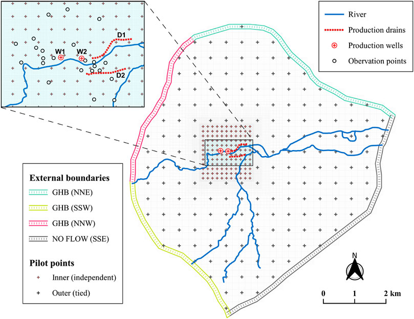
FIGURE 6. Model domain with boundary conditions inferred from the regional groundwater flows. Mesh refinement is conducted in the area of interest around the production and observation wells and drains (see inset). The parameterization of hydraulic conductivity has been conducted with pilot points.

In order to consider contrasting settings while avoiding the burden of transient simulations, pseudo steady-state flow conditions are considered (Haitjema, 2006; Moore and Doherty, 2021). This hypothesis is supported in the present case since the permeable aquifer responds quickly to changes Cousquer (2017). The TrackTools module is used to seed particles around the two wells and the two drains and to derive the mixing ratio of the water withdrawn. It was found that simulated mixing ratios were relatively stable with 500 particles seeded around each production unit (wells and drains). As detailed in Section 2 and references herein, the mixing ratios at source cells where particles stop (β) is inferred from the cell water budget. This allows to account for mixing of aquifer and river water in model cells where a river boundary condition is applied. Note that only the main river is prone to contamination, water originating from the tributaries is not considered as contaminated.

4.2 Parameter estimation and optimization

The model interfacing with the PEST + + suite has been performed by means of PyEMU (White et al., 2016). The hydraulic conductivity field was parameterized with a dense set of pilot points. Hydraulic conductivity values at pilot points lying at the center of the study area were all considered as independent, but they were tied in the outer portion of model domain (Figure 6). This is motivated by the lack of observations in the outer zone and it is unlikely that model predictions are sensitive to details in this remote area.

A series of 10 field surveys, spread over 4 years (2014–2018) have been considered for history matching, considering pseudo steady-state conditions for contrasting stream levels and operating conditions. Though it was challenging for a well field in activity, we have made our best for operating conditions (well discharge rates and drain levels) to remain relatively stable on the period preceding each of the surveys. The observation data set is composed of hydraulic heads, drain discharge rates, and mixing ratios. The latter were derived by end-member analysis from HCO³⁻ and Ca²⁺ concentrations (Delbart et al., 2021).

In order to reduce run times, all model files for each of these surveys were setup in separate folders (Figure 7). Doing so, file operations during parameter estimation were limited to writing parameter files and reading output files. These operations were all conducted with the dedicated methods of the PyEMU Python package.

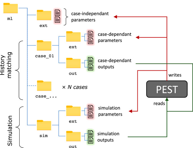
FIGURE 7. Directory tree structure used for parameter estimation and optimization workflow.

The parameter estimation was conducted with the widely used Gauss-Levenberg-Marquardt Algorithm (GLMA) as implemented in PEST + + suite (White et al., 2020b). Parameter increments (DERINC) values were adjusted by trial and error. Best results were obtained with relative parameter increments of 15% for hydraulic conductivities and 10% for all the other parameters. Both zero order (preferred value) and first order Tikhonov regularizations were employed (Doherty, 2015).

After parameter estimation, the resulting model was used to optimize the total abstraction rate. The optimization problem consists in maximizing the total abstraction rate Q while verifying the drinking water quality standards after mixing. It can be expressed as follows:

where the decision variables Q_i and h_i correspond to well discharge rate and drain level, respectively, and the constraint on water quality is expressed as a critical stream-aquifer mixing ratio α_crit.

For this illustrative exercise, the optimization is solved with a sequential version of linear programming as implemented in PESTPP-OPT (White et al., 2018) considering a 50% risk (maximum likelihood) configuration. This algorithm is fast but sensitive to model non-linearity.

4.3 Results

The history matching conducted with the GLMA converged in approximately 10 iterations (Figure 8A). The fit between simulated values with their observed counterparts can be considered as satisfying for heads (Figure 8B) and reasonable for discharge rates and mixing ratios (Figures 8C,D). Measurements of drain discharge rates can be considered as reliable and the misfit may rather be explained by the static, linear relation that is considered with the MODFLOW drain package. In contrast, measurement of mixing ratios derived from concentrations by end-member analysis are prone to uncertainties (Delbart et al., 2021). The structural error of this simplified model is therefore strong and surely contributes to the misfit, but uncertainties in the observation data and historic operating variables are also important. In this context, it is unclear whether more detailed process-modeling could improve the predictive capacity of the model.

FIGURE 8. Results of the parameter estimation with the GLMA. (A) Evolution of the measurement objective function throughout GLMA iterations. Simulated versus measured hydraulic heads (B), drain discharges (C), and mixing ratios (D). Numbers in (B,C,D) refer to the surveys; colors in (B) refer to the observation wells.

The estimated hydraulic conductivity field is highly heterogeneous (Figure 9A), as expected for partly karstified limestones. Attempts to smooth these contrasts with stronger regularization constraints lead to an important increase of the misfit with historical data. Karst conduits are expected to be narrow and of limited extension but can be at the origin of the high values of estimated hydraulic conductivity (Cousquer, 2017). On the opposite, low values can be explained by fine deposits in the riverbed (Delbart et al., 2021).

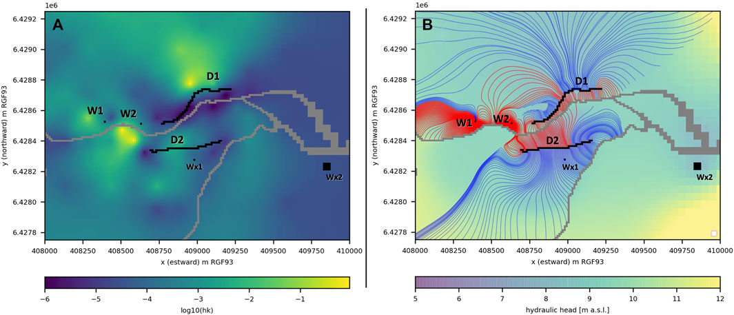
FIGURE 9. (A) Hydraulic conductivity field after parameter estimation. (B) Simulated groundwater table level and particle tracking trajectory for the initial values of parameters Q and α. Particle trajectory from the contaminated stream are colored in red and those from uncontaminated boundaries in blue. Particle tracking was conducted from production wells W1, W2 and drains D1, D2 shown in black. Pumping from wells Wx1 and Wx2 was considered in the flow model but they do not pertain to the studied drinking water facility.

We followed a deterministic approach, which can be considered as a first exploratory step for more robust methods. The “best” calibrated parameter set was therefore used to conduct the optimization of well and drain discharge given a quality constraint expressed as a global mixing ratio α_crit=25%. This corresponds to a 4-fold reduction of contaminant concentration with respect to river contamination levels. The optimization algorithm was run from a situation close to the current operating configuration over three iterations of the sequential linear programming algorithm (Figure 10). Compared to the initial settings (iteration 0), the third and last iteration lead to an increase of production rate by + 25% for a similar contamination level. The particle pathlines for this configuration are presented in Figure 9B.

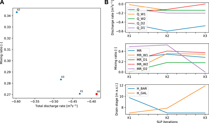
FIGURE 10. Optimization results with (A) total discharge rate and mixing ratio for each optimization iteration of PESTPP-OPT and (B) discharge rate (Q), mixing ratio (MR), and drain stage (H) for each optimization iteration. it0 represents the initial parameter values, it1, it2 and it3 the values for the first, second and third iterations, respectively.

5 Discussion and conclusion

In the context of drinking water contamination issues, we provided a decision-making tool to investigate the vulnerability of groundwater production units. The TrackTools Python module offers pre- and post-processing functions of particle tracking data simulated with MODFLOW and MODPATH. Mixing ratios are inferred from flow contributions of each contaminant source to the discharge rate of a groundwater sink considering particle velocities and mixing in source cells. This can be appropriate where a production well or drain is vulnerable to a boundary condition such as a river. However, the method is not relevant when the source of the contamination is diffuse, such as agricultural contaminants driven by groundwater recharge. In the latter case, forward particle tracking is more appropriate [see e.g., Fienen et al. (2022)].

The synthetic case presented in this work illustrates that contrasting behaviors can be observed even for simple configurations. It highlights the interest of the method to explore the sensitivity of mixing ratios to operating variables (pumping rates, drain levels) and model parameters. The impact of the number of particles seeded around each sink, and the size of the increment used for model linearization was also evaluated through the analysis of the derivatives of α. Derivative instabilities are mitigated when increasing the number of particles or increasing the parameter increment for estimating model derivatives (DERINC). However, adding particles tends to increase the computation time, so that a reasonable particle number should be considered.

Relatively fast and easy to implement, this approach will facilitate the use of contaminant transport models for history matching, uncertainty quantification or optimization. It also presents the advantage to be didactic and can be used to represent contaminant transfer in a visual and potentially interactive manner, which is important for end-users.

The method was implemented on a real world case study and is provided with a series a script for the interfacing with the PEST + + suite. The parameter estimation with the GLMA and optimization by linear programming illustrated the interest of the approach. Difficulties in reproducing observations can be explained by errors in the historic dataset (observations and operating variables) and model structural error. In spite of our efforts to obtain a robust linear version of the model, the methods based on the Jacobian matrix have shown their limitations. This advocates for the use of more robust ensemble methods such as the Iterative Ensemble Smoother (IES (White et al., 2018)) for parameter estimation and uncertainty quantification, and evolutionary algorithms for optimization [PESTPP-MOU (White et al., 2022)]. The presented workflow may easily be extended to these methods recently available in the PEST + + Suite.

The method was illustrated on 2D horizontal models assuming steady state flow conditions. This simplifies the implementation and leads to particularly fast run times, but 3D models and transient conditions may have to be considered in other contexts. The method may be extended to these configurations with some additional processing. The implementation of the method on 3D models will be straightforward so long the wells and drains penetrate a single model layer. Otherwise, particles should be seeded in each of the intersected layers and mixing in the multi-layer well should be accounted considering the respective flow contributions provided by the dedicated Multi-Aquifer Well package (MAW) from MODFLOW6 (Langevin et al., 2017). The impact of transient flow dynamics on the mixing ratio at a specific instant will be easy to consider with backward particle tracking over historic conditions. However, it would be more challenging to quantify mixing ratios averaged over a period as it would require multiple runs of the particle tracking algorithm.

Among the simplifying assumptions of this approach, we assumed the respective flow contributions of particles evenly placed around the sink to be proportional to their velocities (Eq. 1). The validity of this approach has been investigated by Cousquer et al. (2018) with an advective-dispersive model on a synthetic, homogeneous model. Results were encouraging but the performance of the simplified model based on particle tracking may be put into question in other contexts. The use of a paired simple-complex model approach (Doherty and Christensen, 2011) can be suggested, where the complex model would be based on the resolution of the advection-dispersion equation.

Future work will also focus on improving the reliability of the simplified transport models by considering additional processes, such as dispersion. For this matter, various recent particle-based methods (Noetinger et al., 2016; Gouze et al., 2020; Roubinet et al., 2022) and machine learning techniques (Kang et al., 2021; Zhou et al., 2021) could be considered in order to consider more realistic configurations while keeping the low computational cost of the forward models.

As mentioned in the introduction, the optimal complexity level is to great extent, case- and purpose-specific, as it will depend on the purpose of the modeling exercise and the quality of the available observation dataset. In this perspective, it is likely that simple and effective methods such as the one presented in this study remain of interest in numerous situations.

Data availability statement

The datasets presented in this study can be found in online repositories. The names of the repository/repositories and accession number(s) can be found below: https://github.com/tracktools/.

Author contributions

AP: methodology, software development, case study, writing and editing. PM: software development, data processing and visualization. YC: methodology, synthetic case, writing DR: synthetic case, writing, reviewing, editing.

Funding

This work was initially conducted in the framework of the Mhyqadeau project supported by Suez Environnement (LyRE) and the French Aquitaine regional council.

Acknowledgments

The authors are thankful to the editors for handling this special issue and to the two anonymous reviewers for their corrections and valuable suggestions.

Conflict of interest

The authors declare that the research was conducted in the absence of any commercial or financial relationships that could be construed as a potential conflict of interest.

Publisher’s note

All claims expressed in this article are solely those of the authors and do not necessarily represent those of their affiliated organizations, or those of the publisher, the editors and the reviewers. Any product that may be evaluated in this article, or claim that may be made by its manufacturer, is not guaranteed or endorsed by the publisher.

References

M. P. Anderson, W. W. Woessner, and R. J. Hunt (Editors) (2015). Applied groundwater modeling. Second Edition (San Diego: Academic Press). doi:10.1016/B978-0-08-091638-5.00018-3
Asher, M. J., Croke, B. F., Jakeman, A. J., and Peeters, L. J. (2015). A review of surrogate models and their application to groundwater modeling. Water Resour. Res. 51, 5957–5973.
Bakker, M., Post, V., Langevin, C. D., Hughes, J. D., White, J. T., Starn, J. J., et al. (2016). Scripting modflow model development using python and flopy. Groundwater 54, 733–739. doi:10.1111/gwat.12413
Burrows, W., and Doherty, J. (2015). Efficient calibration/uncertainty analysis using paired complex/surrogate models. Groundwater 53, 531–541.
Carniato, L., Schoups, G., van de Giesen, N., Seuntjens, P., Bastiaens, L., and Sapion, H. (2015). Highly parameterized inversion of groundwater reactive transport for a complex field site. J. Contam. hydrology 173, 38–58.
Cousquer, Y. (2017). Modélisation des échanges nappe-rivière à l’échelle intermédiaire : Conceptualisation, calibration, simulation. Ph.D. thesis (Pessac, France: Géoressources et Environnement, Bordeaux INP et Univ. Bordeaux Montaigne).
Cousquer, Y., Pryet, A., Atteia, O., Ferré, T. P., Delbart, C., Valois, R., et al. (2018). Developing a particle tracking surrogate model to improve inversion of ground water – surface water models. J. Hydrology 558, 356–365. doi:10.1016/j.jhydrol.2018.01.043
Daud, M. K., Nafees, M., Ali, S., Rizwan, M., Bajwa, R. A., Shakoor, M. B., et al. (2017). Drinking water quality status and contamination in Pakistan. BioMed Res. Int. 2017, 7908183. doi:10.1155/2017/7908183
de Marsily, G., Delay, F., Gonçalvès, J., Renard, P., Teles, V., and Violette, S. (2005). Dealing with spatial heterogeneity. Hydrogeology J. 13, 161–183. doi:10.1007/s10040-004-0432-3
Delbart, C., Pryet, A., Atteia, O., Cousquer, Y., Valois, R., Franceschi, M., et al. (2021). When perchlorate degradation in the riverbank cannot impede the contamination of drinking water wells. Hydrogeology J. 29, 1925–1938.
Doherty, J. (2010). Addendum to the pest manual. Brisbane, Australia: Watermark Numerical Computing, 131.
Doherty, J. (2015). Calibration and uncertainty analysis for complex environmental modelsWatermark Numerical Computing. Brisbane, Australia.
Doherty, J., and Christensen, S. (2011). Use of paired simple and complex models to reduce predictive bias and quantify uncertainty. Water Resour. Res. 47. doi:10.1029/2011WR010763
Doherty, J. E., and Hunt, R. J. (2010). Approaches to highly parameterized inversion: A guide to using PEST for groundwater-model calibration, vol. 2010. Reston, VA, USA: US Department of the Interior, US Geological Survey.
Doherty, J. (2016). Model-independent parameter estimation user manual part i: Pest, sensan and global optimisers. Brisbane, Australia: Watermark Numerical Computing, 390.
Doherty, J., and Moore, C. (2020). Decision support modeling: Data assimilation, uncertainty quantification, and strategic abstraction. Groundwater 58, 327–337. doi:10.1111/gwat.12969
Fienen, M. N., Corson-Dosch, N. T., White, J. T., Leaf, A. T., and Hunt, R. J. (2022). Risk-based wellhead protection decision support: A repeatable workflow approach. Groundwater 60, 71–86. doi:10.1111/gwat.13129
Gouze, P., Puyguiraud, A., Roubinet, D., and Dentz, M. (2020). Characterization and upscaling of hydrodynamic transport in heterogeneous dual porosity media. Adv. Water Resour. 146. doi:10.1016/j.advwatres.2020.103781
Guthke, A. (2017). Defensible model complexity: a call for data-based and goal-oriented model choice. Groundwater 55, 646–650. doi:10.1111/gwat.12554
Gwimbi, P., George, M., and Ramphalile, M. (2019). Bacterial contamination of drinking water sources in rural villages of mohale basin, Lesotho: Exposures through neighbourhood sanitation and hygiene practices. Environ. Health Prev. Med. 24, 33. doi:10.1186/s12199-019-0790-z
Haitjema, H. (2006). The role of hand calculations in ground water flow modeling. Groundwater 44, 786–791. doi:10.1111/j.1745-6584.2006.00189.x
Hermans, T. (2017). Prediction-focused approaches: An opportunity for hydrology. Groundwater 55, 683–687. doi:10.1111/gwat.12548
Hrachowitz, M., Fovet, O., Ruiz, L., Euser, T., Gharari, S., Nijzink, R., et al. (2014). Process consistency in models: the importance of system signatures, expert knowledge, and process complexity. Water Resour. Res. 50, 7445–7469. doi:10.1002/2014wr015484
Hugman, R., and Doherty, J. (2022). Complex or simple—Does a model have to be one or the other? Front. Earth Sci. 10, 867379. doi:10.3389/feart.2022.867379
Hunt, R. J., Feinstein, D. T., Pint, C. D., and Anderson, M. P. (2006). The importance of diverse data types to calibrate a watershed model of the trout lake basin, northern Wisconsin, USA. J. Hydrology 321, 286–296. doi:10.1016/j.jhydrol.2005.08.005
Kang, X., Kokkinaki, A., Kitanidis, P. K., Shi, X., Lee, J., Mo, S., et al. (2021). Hydrogeophysical characterization of nonstationary dnapl source zones by integrating a convolutional variational autoencoder and ensemble smoother. Water Resour. Res. 57, e2020WR028538. doi:10.1029/2020WR028538
Knowling, M. J., White, J. T., Moore, C. R., Rakowski, P., and Hayley, K. (2020). On the assimilation of environmental tracer observations for model-based decision support. Hydrology Earth Syst. Sci. 24, 1677–1689. doi:10.5194/hess-24-1677-2020
Langevin, C. D., Hughes, J. D., Banta, E. R., Niswonger, R. G., Panday, S., and Provost, A. M. (2017). “Documentation for the MODFLOW 6 groundwater flow model,” in Tech. rep. (Reston, VA, USA: US Geological Survey).
Lien, J.-M., Liu, G., and Langevin, C. D. (2015). GRIDGEN version 1.0: A computer program for generating unstructured finite-volume grids. Reston, VA, USA: US Department of the Interior, US Geological Survey. doi:10.3133/ofr20141109
Moore, C. R., and Doherty, J. (2021). Exploring the adequacy of steady-state-only calibration. Front. Earth Sci. 9, 692671. doi:10.3389/feart.2021.692671
Müller, S., Schüler, L., Zech, A., and Heße, F. (2021). Gstools v1. 3: A toolbox for geostatistical modelling in python. Geosci. Model. Dev. Discuss. 2021, 1–33.
Noetinger, B., Roubinet, D., Russian, A., Le Borgne, T., Delay, F., Dentz, M., et al. (2016). RussianRandom walk methods for modeling hydrodynamic transport in porous and fractured media from pore to reservoir scale. Transp. Porous Media 2016, 1–41. doi:10.1007/s11242-016-0693-z
Pollock, D. W. (2016). User guide for MODPATH version 7—a particle- tracking model for MODFLOW. Reston, VA, USA: U.S. Geological Survey Open-File Report 2016–1086. doi:10.3133/ofr20161086
Pool, M., Carrera, J., Alcolea, A., and Bocanegra, E. (2015). A comparison of deterministic and stochastic approaches for regional scale inverse modeling on the mar del plata aquifer. J. Hydrology 531, 214–229.
QGIS Development Team (2022). Geographic Information System Developers Manual. QGIS Association. Electronic document: https://docs.qgis.org/3.22/en/docs/developers_guide/index.html.
Rajabi, M. M., Ataie-Ashtiani, B., and Simmons, C. T. (2018). Model-data interaction in groundwater studies: Review of methods, applications and future directions. J. Hydrology 567, 457–477.
Razavi, S., Tolson, B. A., and Burn, D. H. (2012). Review of surrogate modeling in water resources. Water Resour. Res. 48. doi:10.1029/2011WR011527
Roubinet, D., Gouze, P., Puyguiraud, A., and Dentz, M. (2022). Multi-scale random walk models for reactive transport processes in fracture-matrix systems. Adv. Water Resour. 164, 104183. doi:10.1016/j.advwatres.2022.104183
Schilling, O. S., Cook, P. G., and Brunner, P. (2019). Beyond classical observations in hydrogeology: The advantages of including exchange flux, temperature, tracer concentration, residence time, and soil moisture observations in groundwater model calibration. Rev. Geophys. 57, 146–182. doi:10.1029/2018RG000619
Schwartz, F. W., Liu, G., Aggarwal, P., and Schwartz, C. M. (2017). Naïve simplicity: The overlooked piece of the complexity-simplicity paradigm. Groundwater 55, 703–711. doi:10.1111/gwat.12570
Sharma, S., and Bhattacharya, A. (2017). Drinking water contamination and treatment techniques. Appl. Water Sci. 7, 1043–1067. doi:10.1007/s13201-016-0455-7
Turner, S. W. D., Rice, J. S., Nelson, K. D., Vernon, C. R., McManamay, R., Dickson, K., et al. (2021). Comparison of potential drinking water source contamination across one hundred U.S. cities. Nat. Commun. 12, 7254. doi:10.1038/s41467-021-27509-9
Valois, R., Cousquer, Y., Schmutz, M., Pryet, A., Delbart, C., and Dupuy, A. (2018). Characterizing stream-aquifer exchanges with self-potential measurements. Groundwater 56, 437–450. doi:10.1111/gwat.12594
White, J. T., Fienen, M. N., Barlow, P. M., and Welter, D. E. (2018). A tool for efficient, model-independent management optimization under uncertainty. Environ. Model. Softw. 100, 213–221. doi:10.1016/j.envsoft.2017.11.019
White, J. T., Fienen, M. N., and Doherty, J. E. (2016). A python framework for environmental model uncertainty analysis. Environ. Model. Softw. 85, 217–228. doi:10.1016/j.envsoft.2016.08.017
White, J. T., Foster, L. K., Fienen, M. N., Knowling, M. J., Hemmings, B., and Winterle, J. R. (2020a). Toward reproducible environmental modeling for decision support: A worked example. Front. Earth Sci. 8. doi:10.3389/feart.2020.00050
White, J. T., Hunt, R. J., Fienen, M. N., and Doherty, J. E. (2020b). “Approaches to highly parameterized inversion: PEST++ version 5, a software suite for parameter estimation, uncertainty analysis, management optimization and sensitivity analysis,” in Tech. rep. (Reston, VA, USA: US Geological Survey). doi:10.3133/tm7C26
White, J. T., Knowling, M. J., Fienen, M. N., Siade, A., Rea, O., and Martinez, G. (2022). A model-independent tool for evolutionary constrained multi-objective optimization under uncertainty. Environ. Model. Softw. 149, 105316. doi:10.1016/j.envsoft.2022.105316
Keywords: particle-tracking, advective transport, steady state, surrogate model, groundwater contamination, stream-aquifer flow, well vulnerability
Citation: Pryet A, Matran P, Cousquer Y and Roubinet D (2022) Particle tracking as a vulnerability assessment tool for drinking water production. Front. Earth Sci. 10:975156. doi: 10.3389/feart.2022.975156
Received: 21 June 2022; Accepted: 29 July 2022;
Published: 25 August 2022.
Edited by:
Michael Fienen, United States Geological Survey, United StatesReviewed by:
Matteo Camporese, University of Padua, ItalyHoward W. Reeves, United States Geological Survey, United States
Copyright © 2022 Pryet, Matran, Cousquer and Roubinet. This is an open-access article distributed under the terms of the Creative Commons Attribution License (CC BY). The use, distribution or reproduction in other forums is permitted, provided the original author(s) and the copyright owner(s) are credited and that the original publication in this journal is cited, in accordance with accepted academic practice. No use, distribution or reproduction is permitted which does not comply with these terms.
*Correspondence: Alexandre Pryet, alexandre.pryet@bordeaux-inp.fr