ArcticBeach v1.0: A physics-based parameterization of pan-Arctic coastline erosion

1 Introduction

Due to warmer temperatures and reduced sea ice protection from bigger waves (Overeem et al., 2011; Casas-Prat and Wang, 2020), especially as freeze-up becomes delayed further into the fall storm season, Arctic coastlines are becoming increasingly vulnerable to the erosion of sandy beaches and destabilization of permafrost cliffs (Biskaborn et al., 2019; Sinitsyn et al., 2020). Large-scale atmospheric patterns have been recently attributed to driving the variability of ice-rich Arctic shoreline erosion (Nielsen et al., 2020) and statistical methods can show promising results to simulate erosion rates (Nielsen et al., 2020). However, current statistical relationships of coastal erosion to other climate variables will change in the future because changes in the Arctic are happening in a non-linear fashion and changes in how tightly certain environmental processes are coupled to erosion is also changing. For example, wave action in the Arctic is increasing nonlinearly, leading to variability of how vulnerable Arctic coastlines are to erosion in the future (Casas-Prat and Wang, 2020). Therefore, understanding the most important root causes of Arctic shoreline change can be only gained through careful evaluation of the physical processes involved. Although extensive process-based models exist (Hoque and Pollard, 2009; Ravens et al., 2017, 2012; Barnhart et al., 2014; Bull et al., 2020) these have only been designed for very specific stretches of coastline and mostly focused on the quickly eroding Drew Point and greater southern Beaufort coastline. These models require extremely detailed initialization data and only pertain to their respective stretch of coastline. These types of models are thus not designed for use on a pan-Arctic level where detailed data on geomorphological characteristics and bathymetry are not available. In addition, notch erosion (undercutting of a steep bluff by water or waves) is a key aspect in their formulation of the coastline retreat process. While this process is important in some geomorphologies along the Arctic, notch erosion does not apply on a pan-Arctic scale (Lantuit et al., 2012). Further, most existing erosion models are computationally expensive and require long run times, not suitable for efficient physical modelling on pan-Arctic erosion scale. Therefore, the need remains to form a physics-based numerical model that can be applied across all partially frozen shorelines. We present, for the first time, a general numerical erosion model that can serve as a starting point for a physics-based parameterization of Arctic shoreline erosion in Earth system models.

The processes involved in Arctic shoreline erosion are different from their mid- and low-latitude counterparts due to the cold temperatures and presence of ice and frozen soils. Shorelines along the Arctic can be frozen and connected to landfast sea ice (Mahoney, 2018), protecting the bluffs and beaches from abrasive wave action. However, strong winds and storm surges can also push ice roughly onto shore, causing erosion, debris influx, and significant destruction of infrastructure and cultural sites (Bogardus et al., 2020). Mitigation measures are necessary in order to protect future disappearance of historical arctic cultural sites in areas impacted by erosion (Nicu et al., 2021). In addition to cultural sites being impacted, erosion will also be detrimental in terms of travel between communities (Irrgang et al., 2019). During the summer, the open water period allows for relatively warmer water to thaw the submerged part of the beach, and warmer air temperatures to thaw the exposed part of the shoreline. Thawing shorelines are especially vulnerable to erosion (Aré, 1988), and climate change accelerates this process due to the lengthening open water season and higher sea and air surface temperatures (Barnhart et al., 2014). Social and economic costs of erosion are high, with entire villages having to relocate (Hamilton et al., 2016; Albert et al., 2018). Nearshore biogeochemistry is also heavily impacted by nutrient-laden sediment supplied into the Arctic Ocean, with roughly one third of the Arctic Ocean primary production supported by riverine and coastal sediment inputs (Terhaar et al., 2021). Further, thawing and eroding coastlines can exacerbate climate change by releasing previously sequestered carbon from the soil into the atmosphere (Vonk et al., 2012; Fritz et al., 2017).

The paper set-up is defined as follows. In Section 2, we describe the erosion model and the physical mechanisms and associated initialization parameters included for simulating the erosion of a partially frozen cliff and beach. Next, we describe the water level model, and how it uses wind forcing to generate a time history of relative water levels at the coastline, which are then used to drive the erosion model. Data used for the validation of both the erosion and storm surge model components are also provided. In Section 3, model results and validation are given, along with model sensitivity to critical parameters. Section 4 and Section 5 provide a discussion of the results and conclusions.

2 Materials and methods

We have coupled the framework of an existing 1-D Arctic coastline erosion model (Kobayashi et al., 1999) with a bathystrophic storm surge model (Freeman et al., 1957), forced by wind speed and direction, and initialized using existing bathymetric information of our study sites. The idealized set-up of the erosion model (Figure 1) includes a beach and cliff profile, assuming uniform conditions alongshore. Conceptually, the model simulates thawing of the beach and cliff sediments according to convective heat transfer controlled by water level and temperature. Thawed material is assumed to be prone to erosion depending on water level and wave action. The process of mass transfer is simulated by emulating a cascade of cliff erosion, beach deposition, and beach erosion. According to the resulting mass balance, the beach and cliff profiles are adjusted assuming constant beach and cliff inclination. A schematic of the main processes and modules of ArcticBeach v1.0 are illustrated in Figure 2.

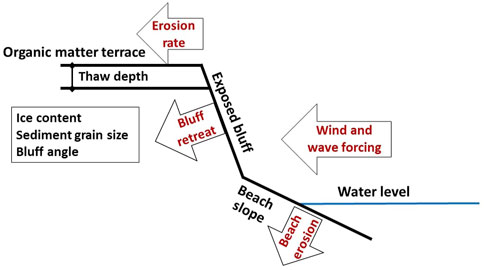
FIGURE 1. Model sketch illustrating basic physical model parameters (black) and processes (red). Wind forcing, masked during times of sea ice cover, is taken from the ERA-Interim reanalysis (Dee et al., 2011) dataset to force a coupled storm surge model. This provides water level data to the erosion model, driving the bluff retreat and beach erosion through a heat and volume balance. Sea surface temperature, wave height, and wave period are also taken into account, as well as the prescribed cliff and beach parameters of volumetric ice content, sediment grain size, cliff height, thaw depth, and cliff and beach angle.

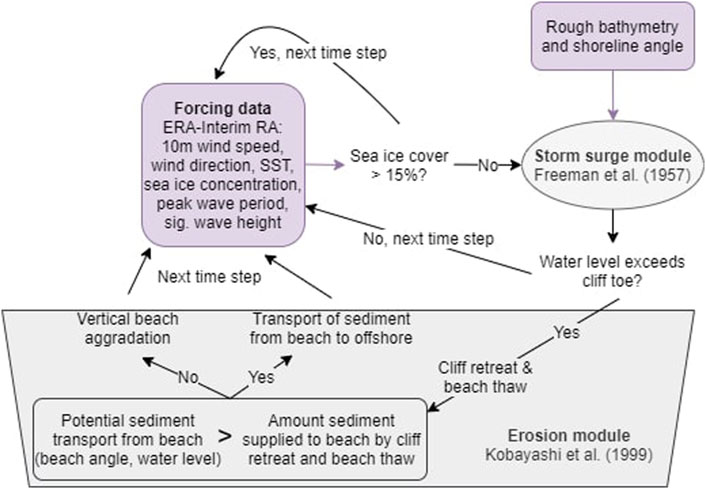
FIGURE 2. A conceptual flow chart summarizing the main inputs (purple) and processes (grey) of ArcticBeach v1.0. Climate forcing and rough bathymetry are used to drive a storm surge module (Freeman et al., 1957). The resulting water levels are then used to drive the erosion module (Kobayashi et al., 1999). A schematic of the erosion module is given in Figure 1. Under times of sea ice cover at the coast (assumed when sea ice concentration exceeds 15%), erosion is assumed to be negligible and neither module is activated.

Small scale processes such as niche formation are accounted for in a bulk tuning parameter (Section 2.5) in this coarse-scale approach. We would like to point out that the model is not aiming for reproducing individual years and erosional events at a specific point, but to deliver large spatial scale and long term (decadal) approximations of coastal erosion related to the physical environmental conditions. This is also the reason why we restricted model tuning to only a single offset parameter. Further description of the beach and cliff model parameters are given in Section 2.1.

2.1 Erosion model

The erosion model used in this study is constructed from heat and sediment volume balances in order to predict horizontal cliff retreat and vertical erosion of a fronting beach. A full description of the framework for this model can be found in Kobayashi et al. (1999), but we provide an overview of the main driving mechanisms here and in the subsequent sections below. Wave action and water levels drive convective heat transfer, and thaw ice-bonded sediments comprising the cliff and beach. When cliff sediment, with its initially prescribed coarse sediment fraction, is released via melting ice between grains of sediment, this coarse sediment is deposited onto the beach, while the remaining fraction of cliff sediment (the fine sediment) is assumed to be transported offshore by the seawater. The amount of coarse sediment (defined by a grain size threshold) that remains on the beach is determined by a volume balance. The volume balance is defined as follows: the rate of coarse sediment transport transported away from the beach cannot exceed a so-called potential sediment transport rate that is determined largely by the beach angle and water level. In general, steeper beach angles and higher water levels lead to higher potential coarse sediment transport rates away from the beach and offshore. Flat beaches and low water levels will result in a low amount of coarse sediment that could be transported offshore. More detail of modelled mechanisms driving cliff and beach erosion are given in the subsequent sections (Section 2.1.1 and Section 2.1.2) and also in Kobayashi et al. (1999).

2.1.1 Cliff erosion

The rate of the cliff retreat is determined by the heat transfer into the exposed frozen cliff face assuming isothermal frozen sediments at freezing temperature (assumed in this study to be 0°C, but can also be adjusted using salinity data near the coastline). The rate of cliff retreat $(\frac{\partial R}{\partial t})$ is, thus, defined by the rate of melting of interstitial ice and subsequent release of cliff sediment determined by the energy supplied divided by the energy required to thaw the part of the cliff face that is exposed to seawater. This expression is given by

where H is the cliff height [m], d_c is the depth of the water level at the cliff toe [m], l_c is the length of the cliff exposed to the water [m], L_c is the volumetric latent heat of fusion [J/m³], B_c is the initial thaw depth on top of the cliff [m], T_w [°C] is the temperature of the seawater, and T_m [°C] is the thawing temperature of the frozen sediment. The parameter h is a convective heat transfer coefficient [J/(s m² °C] between the thawing cliff (h_c) or beach (h_b, Section 2.1.2) surface and warmer seawater. It estimates transfer of heat for a turbulent boundary layer in a unidirectional flow above a flat plate (Schlichting, 1968; Kobayashi and Aktan, 1986) and is given by

where α is an empirical parameter included for wave-induced thawing with α = 0.5 for unidirectional flow, f_w is a wave friction factor at the thawing surface that is dependent on equivalent sand roughness of either the cliff or beach, C_w is the volumetric heat capacity of seawater, and U_b is the representative fluid velocity just outside of the boundary layer and takes into account wave height, wave period, and wave depth. F is a parameter that changes according to thresholds imposed on the Reynolds number, which is directly proportional to the shear velocity accompanying the shear stress on the thawing surface, and changes depending on whether there are hydraulically smooth or fully rough conditions. More detailed information on the convective heat transfer coefficient and relevant parameters including U_b and F are provided by Eqs 10, 11 in Kobayashi et al. (1999). The volume of cliff coarse sediment, per unit width and unit horizontal length, is given by

where P_c is the coarse sediment volume per unit volume of unfrozen cliff sediment [m³/m³], and v_c is the coarse sediment volume per unit volume of the frozen cliff sediment [m³/m³]. The rate of the coarse sediment supplied to the fronting beach is assumed equal to the offshore coarse sediment transport rate per unit width at the cliff toe. Note that this does not allow for accumulation of sediment directly at the base of the cliff. The sediment supply from the eroding cliff (assumed to be zero if water does not reach the cliff), is taken into account when calculating the rate of vertical beach erosion and sediment transported from the beach offshore.

2.1.2 Beach erosion

The potential coarse beach sediment transport rate (i.e., sediment transport from the beach towards offshore) mentioned in Section 2.1 is estimated using available empirical formulas for cross-shore sediment transport on ice-free sandy beaches (Kriebel and Dean, 1985) and adjusted to accommodate a coarse sediment fraction (Kobayashi, 1987). Long-shore transport also defines erosion on sandy beaches but is currently neglected in this 1-D approach. The potential rate of beach sediment is the upper limit for the rate of transport of sediment away from the beach. When the actual sediment transport rate supplied to the beach from the retreating cliff exceeds the potential beach sediment transport rate, then coarse sediment is allowed to accumulate on the beach. However, if insufficient sediment is supplied by the cliff to the beach to accommodate a greater potential transport away from the beach, then no sediment will accumulate on the beach. The balance of both of these processes controls the change in unfrozen coarse sediment on the beach. The change in thickness of unfrozen coarse sediment on the beach is not only determined by the actual transport rate away from the beach and the sediment supply onto the beach from the cliff, but also is influenced by the release of sediment from thawing the beach itself. If the cliff is not providing enough sediment to keep up with the sediment being transported away by the seawater, then the frozen beach is exposed to thaw by the seawater. This results in vertical beach thaw rate defined as $\frac{\partial D}{\partial t}$, as given by

where h_b is the convective heat transfer coefficient on the exposed frozen beach sediment [J/(s m² °C] and is given by Eq. 2, T_w is the temperature of the seawater [°C], T_m is the melting point of the interstitial ice between the sediment grains (which can be adjusted for salinity) [°C], and L_b is the volumetric latent heat of fusion [J/m³]. As long as there is coarse sediment available on top of the frozen part of the beach, the beach is assumed to be protected from thaw and vertical beach erosion does not occur $(\frac{\partial D}{\partial t}=0)$.

To summarize, the change in thickness of unfrozen coarse sediment on the beach is determined by a sediment volume balance controlled by the three major sediment fluxes: 1) the potential offshore beach sediment transport largely determined by beach angle and water level, 2) cliff sediment supply onto the beach, and 3) the release of previously-frozen beach sediment now available for offshore transport due to an increase in beach thaw depth. The change in thickness of unfrozen coarse sediment on the beach, $\frac{\partial B}{\partial t}=0$, is given by

where q_c is the coarse sediment supply rate from the eroding cliff [m²/s] (volume of cliff coarse sediment from Eq. 3 times rate of cliff retreat from Eq. 1), q_melt is the coarse sediment supply rate due to beach thaw [m²/s] over beach width W [m], q_b is the offshore transport rate of unfrozen coarse sediment at the offshore model boundary [m²/s], and P_b is the coarse sediment volume per unit volume of frozen beach sediment.

Consistent with the chosen erosion module in ArcticBeach v1.0, Kobayashi et al. (1999), conductive heat transfer and solar radiation are not directly included. Solar radiation can be partially accounted for in the sea surface temperature input and sea ice cover (see Section 2.3). Conduction effects are much smaller than effects of solar radiation over long time periods and are neglected. However, the opportunity to include effects of solar radiation can be implemented in later versions of the model, to include processes such as thaw slumping and 1-D heat-transfer permafrost models as described in Section 4.2.1.

2.1.3 Validation sites

The validation sites for ArcticBeach v1.0 are Mamontovy Khayata (MK), Bykovsky Peninsula, Siberia, Drew Point (DP), Alaska, United States, and the Veslebogen Cliffs (VC) in Hornsund, Fjord, Svalbard (Figure 3). These sites were chosen because they: 1) involve specialized processes that are, at this time, purposely excluded from ArcticBeach v1.0, and 2) are coastline segments that are very different from each other. We chose not to include the specialized processes of these sites in our simple model because our goal is to establish one general numerical model that represents a first step at simulating diverse types of Arctic coastline, efficient enough to be incorporated into a greater Earth system model. So, to establish this initial model v1.0, we chose these specialized places of MK, DP, and VC in order to test whether or not our model could simulate observed retreat, while, at the same time, not including all of the associated special site-specific processes.

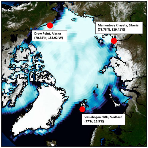
FIGURE 3. Locations of study sites, Mamontovy Khayata, Siberia, Drew Point, Alaska, United States, and the Veslebogen Cliffs in Svalbard.

The differences between the validation sites are highlighted by two main aspects. Firstly, the validation sites differ from each other in terms of their primary erosional processes. At MK, the primary mechanism for erosion is sub-aerial erosion, thermodenudation, and thaw slumping (Günther et al., 2015; Overduin et al., 2016). Coastline retreat at DP, on the other hand, is strongly driven by block erosion (Ravens et al., 2012; Jones et al., 2018). The block erosion occurring at DP is a specialized process that only occurs on very short stretches of Arctic coastline compared to the Arctic coastline as a whole (Lantuit et al., 2012). Unlike the other two sites, the rocky cliffs of VC are not ice-rich because they are not made of soil. While increases in the open water season and storm intensity have been attributed to increased erosion rates in ice-rich permafrost (Barnhart et al., 2014), the erosion processes of rocky cliffs is more complex (Lim et al., 2020). Another reason these validation sites are so different is that they are physically located far away from each other (Figure 3), such that the environmental forcing (sea ice cover, winds, sea surface temperature) are pointedly different. This allows for the model framework of ArcticBeach v1.0 to be tested because it does incorporate all of these forcing variables (which are also readily available from CMIP model output (Meehl et al., 2000) and reanalysis datasets). In this case, these variables were taken from reanalysis data mentioned in Section 2.3.

2.1.4 Cliff and beach parameters

The cliff and beach are each initialized with values for slope, coarse sediment fraction per unit volume for each unfrozen and frozen sediment, sand roughness length (assumed to be 2.5 times the median sediment diameter (Nielsen, 1992)) and initial thaw depth. The beach width and cliff height are also specified at the start of the model run. Default values and reasonable ranges for many of these parameters, taken from referenced literature, were tested in a sensitivity analysis (see Section 2.6). These values, their ranges, and associated references are given in Table 1 for DP and MK. In the case of VC, the cliff height is set to 8 m and ice content is 0.1%. Available parameters from Lim et al. (2020) were used for the reference run.

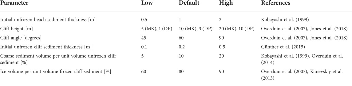
TABLE 1. Parameters used in the Monte-Carlo sensitivity studies to initialize the erosion model are given as “low,” “default,” and “high” values.

2.2 Bathystrophic storm surge model

Due to the extremely limited number of tide gauges spaced across Arctic coastlines, we provide water level to our erosion model by coupling a bathystrophic storm surge model (Freeman et al., 1957; Dean and Dalrymple, 2004) forced by globally-available reanalysis winds (Dee et al., 2011). This model provides water level data based on wind speed, wind direction, coastline angle, and bathymetry. Coastline angle and bathymetry are assumed to remain constant alongshore. The model is quasi-static, and solves reduced equations of motion for storm surge, induced by wind stress and the Coriolis force. The governing equations are given by

where x and y are directed onshore and alongshore, respectively, g is gravitational acceleration [m/s²], h is mean water depth [m], η is the deviation from mean water depth [m], f is the Coriolis frequency [1/s], τ_s and τ_b are surface wind and bottom stresses respectively [kg/(m s²)], and ρ is density of seawater [kg/m³]. In the first equation, hydrostatic forces from the storm surge (also referred to in this study as relative water level) in the x-direction (onshore) are balanced by flow V in the y direction (alongshore), and also the wind shear stress component in the onshore direction. In the second equation, the inertial force in the alongshore direction are balanced with alongshore wind surface and ocean bottom shear stresses, which are found using a drag law (Dean and Dalrymple, 2004). Quasi-static conditions are assumed, such that $\frac{\partial V}{\partial t}=0$ and onshore flow U is neglected (set to zero). The above equations are solved using a finite difference scheme, and essentially produce a time history of relative water level elevation as a function of changing wind stress.

2.3 Model forcing

The forcing for the storm surge model and erosion model comes from the ERA-Interim reanalysis dataset (Dee et al., 2011). Specifically, the 10 m east and west wind speed vectors are used to force the storm surge model, and the sea surface temperature, peak wave period, and significant wave height are used. Winds and sea surface temperature have a 3-hourly temporal resolution. Wave period and significant wave height have a 12-hourly and 6-hourly resolution, respectively. All of these variables were interpolated into hourly timesteps. Changes in wave height, wave period, and sea surface temperature are accounted for when convective heat transfer between the ocean and cliff/beach is calculated by the erosion model (Kobayashi et al., 1999).

When the winds force the storm surge model, it provides water levels on the beach and at the cliff toe for the coupled erosion model. The vector averages of wind speeds and direction over the open water season were also calculated to help analyze the output of the model. The ERA-Interim variables were extracted from the grid cell nearest to each study site.

Since most Arctic erosion occurs during the summer when the coasts are exposed to thermal abrasion by wave action, we use only forcing data over the open water season. To mask the forcing over the ice-covered period, we extracted sea ice concentration from the same grid cells offshore the study sites (Figure 3). When the sea ice concentration had a value of 15% or more, the winds, wave, and sea surface temperature information were masked. Winter storms can occur over less than 15% sea ice cover, so when this happens, erosion is still simulated during winter.

2.4 Validation data

Observations of water level were used to validate the storm surge model output. The observed water levels at the MK study site were collected in the summer of 2007, 2008 every 15 min by a water level gauge (Scheller, 2012). The water levels were averaged to a 3 h mean, and the mean of the total time series was subtracted from each timestep value, so that the variability oscillated around 0 m (representative of mean sea level). Monthly tide gauge values are available at nearby Tiksi, but the monthly temporal resolution is not frequent enough to provide meaningful validation of water level values or force ArcticBeach v1.0. However, tide gauge data of a higher frequency (hourly) is available at Prudhoe Bay, Alaska, which is near the other case study site of DP, Alaska (NOAA, 2022). The raw tide gauge data is recorded roughly every 6 min and was downloaded as hourly averages. The tide gauge data were further averaged to a 3 hourly mean to correspond with the 3-hourly mean ERA-Interim wind forcing, and then compared to the modelled water level data. To validate the retreat rates, observations of bluff erosion at DP were used (Jones et al., 2018), as well as observed retreat rates at MK on Bykovsky Peninsula (Grigoriev, 2019). Observations of cliff erosion at VC for the period of 2014–2016 were taken from Lim et al. (2020). No tide gauge data is available at VC, but was not required because sufficient validation of the storm surge model was performed from the observed water levels at the other two sites.

2.5 Model calibration

The beach profile along even short stretches of coastlines are highly variable (Overduin et al., 2014), and changes in beach profile directly influence how much water reaches the backing cliff face. Cliff retreat is not activated in the model unless the water level reaches the cliff. Therefore, retreat rates are highly dependent on the water levels reaching the cliff. We have calculated a so-called ‘water level offset’ that is required for the coupled erosion-storm surge model to reproduce observed erosion rates at each site. This offset is required for two main reasons. The first is that the absolute water depth at the cliff toe (Figure 4) is not known at the study sites, only the water depth relative to local tide gauge datums (where tide gauges are available) are known. The storm surge model calculates water levels relative to still water (no winds) only, which is a reference point that does not exist in reality. The second reason we calculate a water level offset is that it acts as a bulk correction parameter since the model so far only includes primary drivers of Arctic coastal erosion, while secondary physical processes remain to be added, such as thaw slumping and sub-aerial erosion (Overduin et al., 2014). Aside from compensating for the unknown absolute water level depth, the water level offset can be interpreted as a proxy for the unresolved physical processes driving erosion of Arctic shorelines.

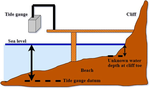
FIGURE 4. Schematic of a reference level for a tide gauge while indicating the water level depth at cliff toe remains unknown due to unknown bathymetry on scales of less than 0.5 m. In this approach, extremely detailed bathymetry information, as well as tide gauges along the entire Arctic coastline, would be required to know the water depths at the cliff toe, which is not feasible. To calibrate ArcticBeach v1.0, our water level offset approach using simulated water level values in response to changing wind speed and direction integrates this issue.

The water level offset was calibrated from annual observed retreat rates for each study site, using a non-linear numerical solver (SciPy.org, 2022) with a relatively low initial guess of 0.2 m. The offset values were calculated for each year, and the median of the offset from the yearly time series was saved. This median offset value for each site was added to the water levels calculated by the storm surge model. This sum (water level offset plus modelled water level variability) was then used as the time series of water level forcing for the erosion model. When the annual water level offset exceeds the median of the entire water level offset timeseries, it follows that the modelled retreat will be underestimated for that year, and vice versa. This is due to the calibrated summed water level that is applied to simulate erosion being lower than the annual water level necessary to reproduce the exact erosion rate for the given year.

2.6 Monte Carlo sensitivity tests

In order to test the sensitivity of the modelled retreat rates, a Monte Carlo approach was used with varying beach and cliff parameters. Each parameter was assigned a realistic range of values, and randomly assigned a value that was within a uniform distribution of this range. We chose a uniform rather than a central distribution because it provides a more comprehensive assessment of error, given that observations are relatively few and so we cannot confidently assess prior probability distributions. The Monte Carlo sensitivity studies were only performed for the sites of DP and MK because the centimeter scale of erosion at the rocky VC site was deemed too small for meaningful results. For each year, 500 simulations were performed, with the randomly assigned parameter kept constant across all years examined, for each study site during its respective simulation. When the sensitivity of the parameter was not being tested, it was assigned its default value, set according to literature. The default values of these parameters and the referenced ranges that were tested are provided for MK and DP in Table 1. To further illustrate our Monte Carlo method, we will use the example of how changes within a uniform distribution of observed ice content can be expected to change the modelled retreat rates. We ran ArcticBeach v1.0 a total of 500 times for each site, and for each model run, a certain percentage of cliff ice was assigned to a different value each time but within the observed range of 60–90% (given in Table 1). In this example, since all other parameters remained unchanged except ice content, this resulted in a distribution of retreat rates caused by changes in cliff ice content.

3 Results

3.1 Modelled and observed retreat

Observed retreat rates vary from 1.3–11.0 m/year at MK, 6.7–22.6 m/year at DP, and only 0.01–0.019 m/year at VC (Figures 5A–C respectively). The retreat rates shown in a cumulative form (Figures 5D–F for MK, DP, and VC respectively) give a good overview of general model performance on longer timescales, and have been calculated for those years annual observed retreat rates are available.

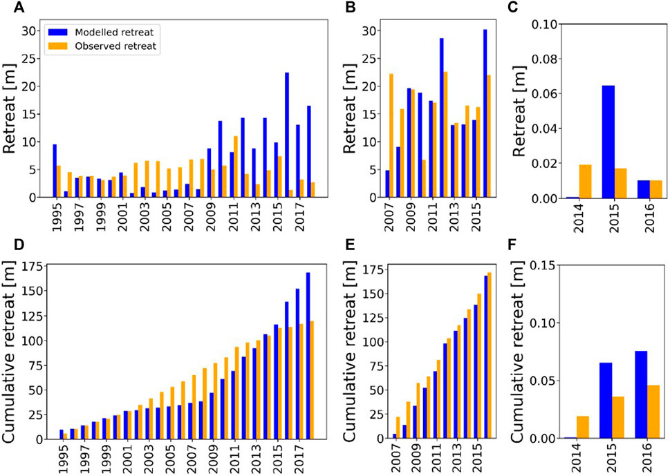
FIGURE 5. Observed (orange) and simulated (blue) annual bluff retreat rates (A–C) and cumulative retreat rates (D–F). Values for Mamontovy Khayata are given in (A,D), Drew Point in (B,E), and Veslebogen (C,F). Note the different scale for the y-axis for the Veslebogen site. The years when the observed retreat rates are under (over)-estimated are the same years when the annual values of the so-called “water level offset,” a proxy for the physical processes at this point unresolved by the model, are above (below) the median values. These years are indicated where the red star is above (below) the red dashed line in Figure 9.

Over the period where annual observations exist, the cumulative retreat rates for the ice-rich coasts agree better with the cumulative modelled retreat at DP (within a few meters) than at MK (roughly 40 m). However, good performance (within a few meters) of individual years can be found for both sites. The frequency of when the model overestimated or underestimated observed retreat followed somewhat of a pattern in MK, where it did not at DP. This over- and underestimation is expected when we examine the annual water level offset values in comparison with the median water level offset value that was used in model calibration (Section 2.5). For example, during the early years of the data record at MK (1997–2001), the model agrees well with the observations (error less than 1 m), but in the middle period of the time series (2002–2008), the model underestimates observations, and in the later years (2009–2018) the model overestimates observed retreat. This causes cumulative simulated retreat time series to resemble an exponential curve, while the observed cumulative retreat has a more linear curve (Figure 5C). To further illustrate how we can expect when the model will over or underestimate observed retreat, we will take the example of the underestimation of coastline retreat at MK during the period of 2002–2008 (Figure 5A). This underestimation of retreat is caused by the annual water level offsets calculated for 2002–2008 being above the median water level offset used in the model forcing (see red stars above the red dashed line for 2002–2008 in Figure 9A). This means that the calibrated water level required to reproduce the observed retreat for 2002–2008 is higher than the median of the calibrated water level to reproduce the observed retreat across the entire timeseries. While bulk calibration inevitably leads to errors for individual years, we find this approach is still able to capture cumulative retreat over a long timeseries well (Figures 5C,D). The root mean square error (RMSE) of simulated coastline retreat for MK is 7.84 and 7.23 m for DP (Table 2).

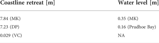
TABLE 2. The root mean square error (RMSE) of simulated coastline retreat and water levels for the study sites. At DP, no observed water levels are available, so the water levels from the nearby tide gauge at Prudhoe Bay were used, as described in Section 2.4. Prior to calculating the RMSE of modelled water levels at Prudhoe Bay, the mean offset between the modelled and observed water level was first removed because the water level observations and water level model correspond different baselines (see Section 2.5). Tide gauge data is not available at VC but not necessary since validation of the storm surge model is provided by the other two sites.

For the rocky site of VC, the cumulative retreat for the time period of 2014–2016 is 0.046 m, while the modelled retreat is 0.075 m, leaving the difference at 0.029 m. This shows that ArcticBeach v1.0 is able to reproduce the same order of magnitude for this small amount of erosion of the rocky cliffs on the scale of 1 cm but also on the order of 10 m for the ice-rich permafrost cliffs of DP and MK. The RMSE of the simulated rocky cliff retreat is 0.029 m (Table 2).

3.2 Storm surge model performance compared to tide gauge data

The storm surge model, providing the water levels due to changing wind conditions to our erosion model, reproduces the observed water level variability relatively well at both locations (Figure 6). Unlike the simulated water levels, the reference baseline for Prudhoe Bay tide gauge data (blue line in Figure 6B) is mean sea level. Mean sea level does not correspond to a water depth with no winds (which is the reference for our simulated water levels) because mean sea level is also influenced by local currents and larger-scale ocean circulation (e.g., the Alaska coastal current (Talley, 2011) and the Beaufort Gyre at DP). Observed water levels at MK (blue line in Figure 6A) were taken from a depth relative to where the water depth sensor was deployed, which was around 11 m from the surface (Scheller (2012) and Section 2.4). To compare the variability between the simulated and observed water levels at MK, the baseline of the water level sensor has been set equal to the baseline (relative to 0 m) of the simulated water levels. Bathymetries with a very high spatial resolution are not required for water level simulations. This could prove advantageous for use in areas where nearshore bathymetry must be approximated due to insufficient data. In MK, the water level model is able to reproduce the pattern of observed water level, with the exception of very high peaks and very low troughs (Figures 6A,C) The range of the modelled water levels is 1.2 m and the range of observed water levels is 2.7 m, with a significant correlation of 0.40. In contrast, at Prudhoe Bay, 3 hourly means of available tide gauge data (recorded roughly every 6 min, averaged over every hour) from 2007–2016 consistently gave less extreme highs and lows compared to the simulated data (Figure 6D). Since the Prudhoe Bay tide gauge provides values relative to mean sea level, and the storm surge model provides water level values relative to still water depth, an offset between the two datasets is expected. For example, in 2007, the simulated water level values were consistently lower than the observed water level values, but the 3-hourly variability was still well captured. The range of the modelled and observed water levels are similar, at 1.1 and 1.0 m, respectively, with a significant correlation of 0.64 (Figure 6B). The RMSE for the storm surge model at the MK is 0.35 m. For Prudhoe Bay, the RMSE was calculated after removing the mean offset caused by a different relative baselines described above and was found to be 0.16 m (Table 2).

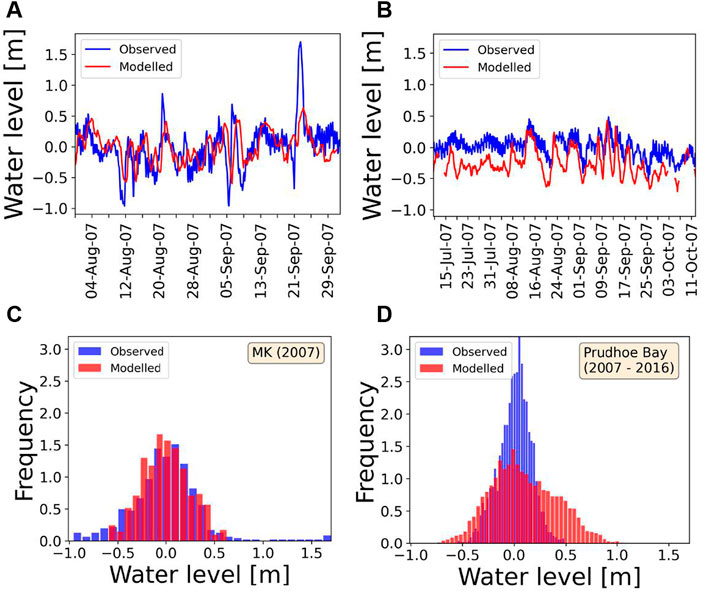
FIGURE 6. Comparison of modelled (red) and measured (blue) water levels. The forcing for the modelled water levels is masked based on sea ice concentration (resulting in a different time period analyzed at each site) and is from the respective offshore ERA-Interim grid cell closest to where the water level validation data was measured near each study site. The modelled water levels have an offset applied such that the mean modelled water level is equal to the observed water level for a,c, and d. In (A) The observed water levels near the MK site are taken from a one-time deployment of a water depth gauge at 71.53°N, 129.56°E in 2007 (Scheller, 2012). In (B) the observed water levels (blue line) are from the Prudhoe Bay tide gauge (near DP), with data from the year 2007 relative to mean sea level given here as an example, with the corresponding modelled 2007 water levels (red line) relative to a theoretical still water depth. (C) shows the frequency of the modelled and observed water levels for MK (comparison only available for 2007) and (D) the full erosion period studied for DP (2007–2016).

3.3 Coastal winds and modelled water levels

The storm surge model is primarily driven by changes in wind stress. In the Northern Hemisphere, when winds are primarily directed toward the left (as observed from the beach) alongshore or directly offshore during the open water season, a relatively low water level is expected due to the Coriolis force and wind stress working to push water offshore. This effect becomes apparent during the 2007 open water season at the north-facing coastline of DP, when the winds were most frequently directed offshore (Figure 7A, left panel). This offshore wind pushed the water away from the coast, resulting in an average water level negative relative to what it would have been in calm conditions (Figure 6B and left panel of Figure 7B). In the 2009 open water season at DP, offshore winds were less frequent, while more frequent and stronger north-northeasterly winds (Figure 7A, right panel) allowed some water to accumulate closer to the beach, but still produced a mean negative value (Figure 7B, right panel). Winds coming from northeasterly directions in 2009 is more typical of DP than offshore southeasterly winds that were observed during the open water season in 2007. Both years had roughly the same open water season, but unlike the “clean” and well-defined open water period of 2009, 2007 had a false break-up in mid July, as well as a false freeze-up near the end of October (black line in Figure 7B, left panel). A false break-up occurs when ice melts out or breaks off the coast, and then forms or drifts in again before the longer open water season. A false freeze-up is similar, when the ice forms or drifts in at the coast but then returns to open water before the longer ice-covered season (Rolph et al., 2018).

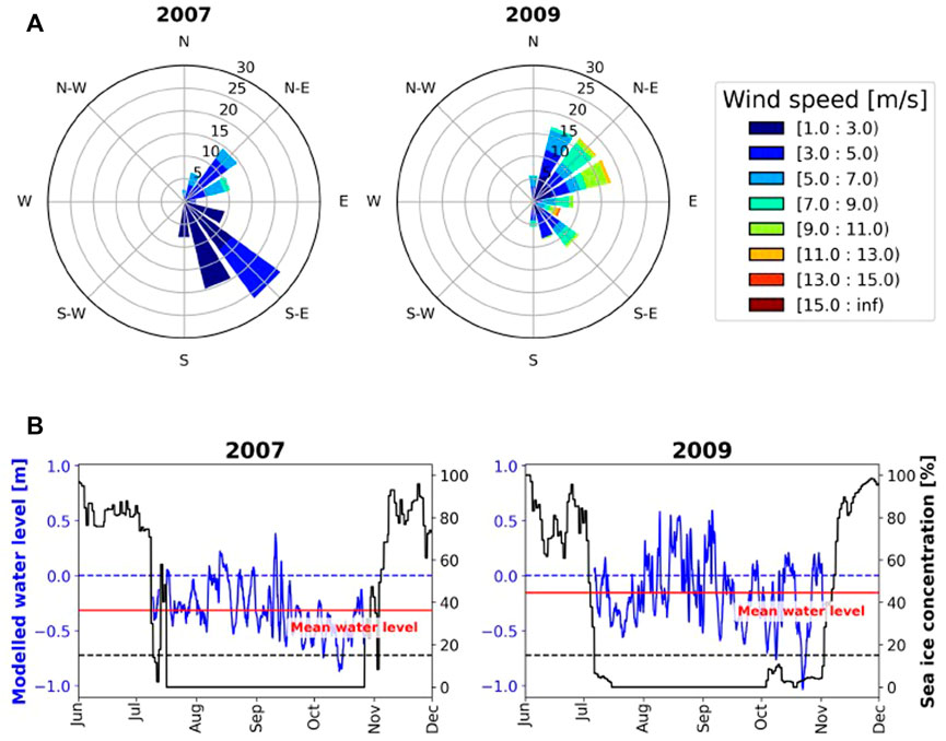
FIGURE 7. Frequency of wind speed and direction (A) with corresponding modelled water levels and sea ice concentrations (B) for selected years at Drew Point. Wind directions are vector-averaged over the open water season. The open water season is defined when the sea ice cover (black line) is below 15% (black dashed line). Wind and sea ice data are taken from ERA-Interim reanalysis.

The MK coastline faces northeast. So, northeasterly winds should generally push water towards shore, raising the water levels near the coast. Onshore winds are more frequent at MK (Figure 8A), compared to winds at north-facing DP (Figure 7A). Consequently, water levels simulated at MK forced under these winds are higher than at DP (compare red mean water level lines in Figures 7B, 8B). The 1999 open water season was roughly twice as long compared to 2002. The open water season was relatively well-defined in 1999 except for 1 false break-up event at the end of June, while 2002 had 14 short false break-up and freeze-up events scattered throughout its short open water season (black lines in Figure 8B).

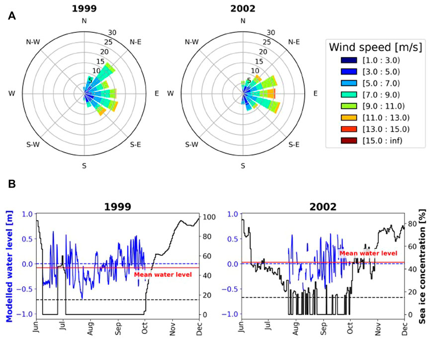
FIGURE 8. Frequency of wind speed and direction (A) with corresponding modelled water levels and sea ice concentrations (B) for selected years at MK. Wind directions are vector-averaged over the open water season. The open water season is defined when the sea ice cover (solid black line) is below 15% (dashed black line). Wind and sea ice data are taken from ERA-Interim reanalysis.

3.4 Variability of water level offsets over a changing open water season

Variability of the open water season during the years with observed retreat rates is higher at MK than at DP (blue bars in Figure 9). At MK, the open water season ranges from 52–133 days, and at DP, from 86–133 days. Similar to the duration of the open water period, the variability of the derived water level offset is found to be higher at Mamontovy Khataya than at DP (red stars in Figure 9). The range of the water level offset for MK is -0.2–2.2 m, and 0.2–1.0 m for DP. Due to the more positive skew of water level offsets at MK, the median water level offset (the final calibration value used to force the model) is further from the mean water levels at MK in comparison to the nearly equal median and mean water level offsets at DP (compare distances between the black solid and red dashed lines at each of the two sites in Figure 9).

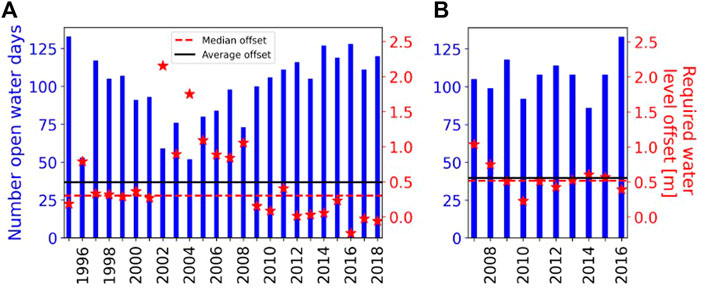
FIGURE 9. The number of open water days (number of days sea ice concentration is below 15%) for (A) Mamontovy Khayata and (B) Drew Point. The average (black line) and median (red line) of the water level offsets for (A) Mamontovy Khayata and (B) Drew Point, required for the model to reproduce observed retreat rates. When the annual water level offsets (red stars) exceed the median water level offset (red dashed line), the model predictably underestimates observed retreat rates (see corresponding years in Figure 5) and vice versa.

3.5 Sensitivity to critical model parameters

The sensitivity of the model was analyzed regarding uncertainties for individual parameters including cliff height, cliff angle, and ground ice content. Furthermore, a full uncertainty test was performed within which multiple model parameters (see Table 1) were varied within physically reasonable ranges.

The simulations for DP showed a higher sensitivity of retreat rates to changes in cliff height than the simulations for MK (Figure 10). In general, higher sensitivity of retreat rates to changes in cliff height occurs in the location with the lower initially-prescribed cliff height (DP). At MK, years with higher retreat rates simulated during typical conditions (defined in Section 2.6) show a higher sensitivity of retreat rate to a changing cliff height (1995, 2009–2018 in Figure 10A) than years with lower simulated retreat rates during typical conditions (1996–2008). At both locations, there are noticeably more outliers overestimating retreat rates than outliers underestimating retreat rates. At DP, the average interquartile range of retreat rate sensitivity to changes in cliff height (Figure 10B) was roughly 10 m and relatively consistent across all years tested, with the exception of 2007 which had a low modelled retreat rate under default parameters. Sensitivity of retreat rate changes in cliff angle is smaller than that of change in cliff height for both study sites (Figure 11). When the simulated retreat rates using default parameters were low (e.g., 1996–2008 at MK, and 2007 at DP, indicated by the blue dots in Figure 11), then the sensitivity to the cliff angle is also low. Sensitivity of retreat rates changes in cliff ice content is similar to that of cliff angle for both sites (Figure 12). While still within the same order of magnitude, the observed retreat rates mostly lie outside of the interquartile range given by all sensitivity tests. This is also true for the full uncertainty runs, where cliff height, cliff angle, unfrozen cliff sediment thickness, coarse sediment volume per unit volume of unfrozen cliff sediment, and cliff ice content were allowed to vary (Figure 13, Table 1).

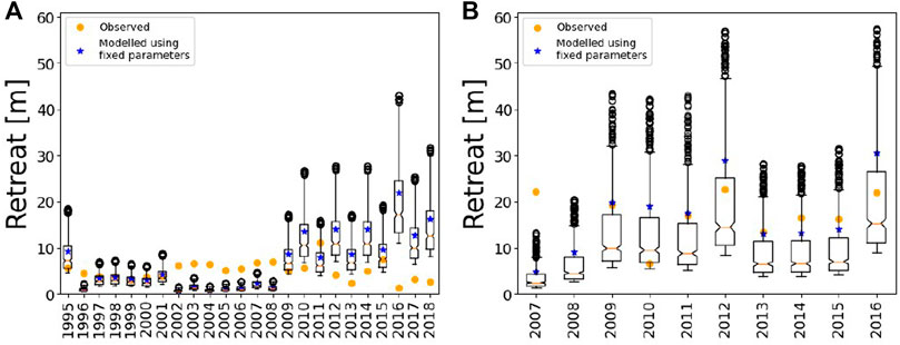
FIGURE 10. Erosion rate sensitivity from changes in cliff height for (A) Mamontovy Khayata and (B) Drew Point. Blue dots indicate the retreat rates simulated under fixed model parameters. Orange dots indicate retreat rates based on observations.

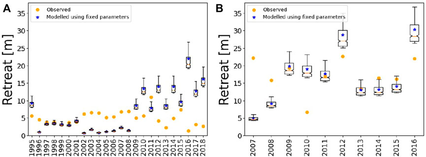
FIGURE 11. Erosion rate sensitivity to changes in cliff angle for (A) Mamontovy Khayata and (B) Drew Point. Blue dots indicate the retreat rates simulated under fixed model parameters. Orange dots indicate retreat rates based on observations.

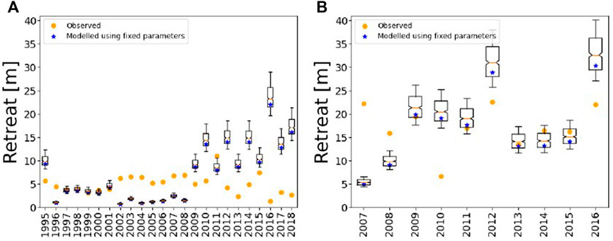
FIGURE 12. Erosion rate sensitivity to changes in cliff ice content for (A) Mamontovy Khayata and (B) Drew Point. Blue dots indicate the retreat rates simulated under fixed model parameters. Orange dots indicate retreat rates based on observations.

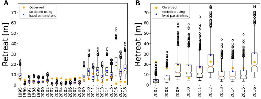
FIGURE 13. Erosion rate sensitivity to changes in cliff height, angle, unfrozen sediment thickness, coarse sediment volume per unit volume of unfrozen sediment, and ice content for (A) Mamontovy Khayata and (B) Drew Point. Blue dots indicate the retreat rates simulated under fixed model parameters. Orange dots indicate retreat rates based on observations.

4 Discussion

4.1 Effects of calibration on simulated retreat rates

The simulated retreat rates of DP and MK (Figure 5) are highly sensitive to the calculated water level offset forcing (Section 2.5 and red stars in Figure 9). The variability of the simulated water levels and open water season length directly influence model performance of reproducing observed retreat rates. This agrees well with the results of Barnhart et al. (2014) and Islam et al. (2020) such that Arctic erosion rates of ice-rich coasts are highly sensitive to ocean water level. An important tuning parameter of our erosion model is the median of the so-called water level offsets that were calculated from a yearly time series (see Section 2.5). A higher skewness of the yearly offset value will naturally result in a median value less representative of the individual yearly points. This is demonstrated, for example, by the median value (red dashed line in Figure 9A) being less representative of individual offsets (red stars in Figure 9A) at MK than at DP, where the median value matches the yearly offsets well (Figure 9B). Essentially, since this median value (Section 2.5) is then added to the simulated water level variability driven by changes in wind speeds and direction (Section 2.2), how well the median matches the individual, yearly calibrated values will directly reflect model performance during individual years. Indeed, we can see that the retreat rates modelled for DP (the location where the median offset is closer to the mean of the calibrated offset values of individual years) match observed retreat better than at Mamontovy Khayta (Figures 5C,D). The water level offset for VC was very small (order of centimeters) and this is due to the ice content of the cliffs being low and so not as sensitive in the model to water level forcing.

4.1.1 The impact of wind direction on modelled water level and erosion

Unchanging wind vectors result in a constant modelled water level. Given similar open water season lengths, low annual variability in wind speed and direction will result in similar simulated water levels. The water level offset, a tuning parameter used in this model (Section 2.5), is a function of observed retreat rate and wind vectors over a changing open water season. Since the same tuning value (the median of the annually calculated water level offset, per study site) is used across all years, we can expect ArcticBeach v1.0 to perform better in locations where the median and mean of the annual values used to calculate the tuning parameter are similar. In other words, the skewness of the annual water level offset time series can be a predictor of how well ArcticBeach v1.0 will perform at a given location. At DP, for example, the lower variability of the open water season compared to MK (Figure 9) results is a less positive skew of the water level offset, causing ArcticBeach v1.0 to simulate observed retreat rates better at DP (Figure 5). Causes for low skewness in the annual water level offset time series could be a more consistent open water season, along with persistent wind speeds and directions, as well as low variability in observed retreat rates. Therefore, ArcticBeach v1.0 will perform best at a coastline that meets these conditions. However, since the tuning parameter is a function of all these different conditions, changes in one aspect can be compensated for by changes in another. For example, given the same observed retreat rate, a similar water level offset would be calculated for a short open water season but strong winds pushing water onshore as a season with a longer open water duration but calmer winds. To describe this idea in more detail, we now analyze the performance of ArcticBeach v1.0 using the examples of individual years at our two study sites, taking into account the length of the open water season, wind direction, and mean modelled water levels.

ArcticBeach v1.0 simulated the observed retreat rates almost exactly in 2009, while underestimating retreat rates by roughly 23 m in 2007 (Figure 5B). Taking a closer look at the wind directions during these years, the primarily southeasterly winds during the open water season in 2007 (left panel, Figure 7A) push water away from the DP coast more effectively than the stronger, primarily northeasterly winds of 2009 (right panel, Figure 7A). Given that the duration of the open water season is similar in both 2007 and 2009 (Figure 9B), the differences in wind direction explain why the average modelled water levels in 2007 are lower than in 2009 (Figure 7B). Since the median of the annual time series of the water level offset (Figure 9B) is closer to the average modelled water level value in 2009 than it is in 2007, this results in a better performance of ArcticBeach v1.0 in 2009 compared to 2007.

At MK, the erosion model underestimates the observed retreat rate of 7 m in 2002 by roughly 6 m, while successfully reproducing the observed retreat of roughly 4 m in 1999 (Figure 5A). In contrast with the similar open water season length at DP in our example years of 2007 and 2009 described above, the length of the open water season at MK for 1999 is slightly less than half of the open water season of 2002. Also, in contrast with our example years at DP, the wind directions in 1999 and 2002 over the open water season are similar at MK in both speed and direction (Figure 8A). This results in a similar modelled mean water level in 1999 and 2002, and therefore a similar difference to the median water level offset added to the modelled water level variability used to force the erosion model. However, due to the significantly shorter open water season in 2002 (Figure 8B), the cumulative water level reaching the cliff and therefore available to cause erosion during the open water season is much less in 2002 than in 1999. The much shorter open water season understandably leads to a higher required water level offset for the model to reproduce observed retreat, much higher than the median of the offsets over all years (Figure 9A). This large difference between the modelled average water level and median required water level offset result in an underestimation of observed erosion in 2002 at MK. These examples illustrate how ArcticBeach v1.0 performs under years of variable open water seasons, and suggest that under a more uniform open water season length, ArcticBeach v1.0 will simulate observed retreat closer to reality. With a pack ice cover retreating to the north, including the area of partial sea ice cover (Rolph et al., 2020), we can expect the open water season to become more uniform in duration, and subsequently expect the current setup of ArcticBeach v1.0 to perform better under projected climate conditions.

4.2 The impact of geomorphological cliff and beach parameters on modelled erosion retreat rates

Due to the computationally inexpensive and fast nature of ArcticBeach v1.0, our model can provide a quick and useful tool about which parameters (e.g., cliff height, ice content) are the most important in influencing the rate of cliff retreat. This can be particularly useful to help design experiments for physical wave tank models of partially frozen beach erosion (Korte et al., 2020). Sensitivity of erosion rates to changes in cliff parameters is high (Figures 10, 11, 12, 13). At VC, the very low ice content in the cliffs resulted in very small retreat rates (Figure 5). Sensitivity of retreat rate to changes in ice-rich cliff height is also understandably influenced by the ratio of water level change to total cliff height. This is shown by the lower sensitivity to changes in cliff height at the prescribed higher cliffs at MK (Figure 10A), compared with the higher sensitivity of retreat of shorter bluffs found at DP (Figure 10B). Given short bluff heights and high water level forcing, the rate of retreat will tend to increase, as expected by Eq. 1 and shown in Figure 10. During years where the median water level offset of the full time series is higher than the annual offset (e.g., in 1995, 2009, 2010, and 2012–2018 at MK, Figure 9A), the cliff length exposed to seawater (distance of the cliff submerged in seawater from the cliff toe upwards) is overestimated in the final model forcing (Section 2.5). Therefore, changes in cliff height (H) will result in a greater change in $\frac{\partial R}{\partial t}$ when the cliff length exposed to seawater (l_c) is larger (Eq. 1). This length is directly proportional to the level of convective heat transfer and thaw of the cliff itself, resulting in retreat (See Section 2.1.1 and Eq. 1). Indeed, the highest sensitivities of retreat due to changes in cliff height occur during those years where the median water level is higher than the annual water level offset at Mamontovy Khayta (1995, 2009, 2010, and 2012–2018, Figure 9A).

Cliff angle is important in our simulations of erosion rates because the angle of the cliff (given the same water depth at the cliff toe) determines the length of the cliff exposed to the relatively warmer seawater, influencing the level of convective heat transfer and subsequent cliff thaw. Similarly, the ice content of the cliff is also directly proportional to how effective the convective heat transfer applied to the cliff is at thawing the cliff sediment, releasing it onto the beach for subsequent transport offshore (Eq. 1). This process is particularly apparent at DP, where changes in cliff ice content are more influential on erosion rates than at MK (Figure 12) because seawater covers a greater fraction of the shorter cliffs prescribed at DP than at the higher cliffs MK (Table 1). As found in Hequette and Barnes (1990), cliff and beach parameters alone cannot explain the observed erosion rates, which agrees with our sensitivity test results in this study. Sea ice gouging, for example, can play an important role in nearshore erosion and accretion (Hequette and Barnes, 1990).

4.2.1 Water level offsets as a proxy for unresolved processes

The variability and magnitude of the water level offset (Figure 9) is also a proxy for how much the processes that are not included in the model (e.g., sub-aerial erosion and thaw slumping) play a role in determining the observed retreat rate. A thermal heat flux model, such as CryoGrid (Westermann et al., 2016), can be used to identify the changing thaw depth of the bluff which is currently a constant in the model. Further investigation is required to derive either an empirical or physical estimate of thaw slumping rates as a function of changes in thaw depth. However, calibration from existing slumping observations (Lantuit and Pollard, 2008) in conjunction with CryoGrid output over the same time periods could lead to such a result. This empirical or physical function would then be incorporated into the rest of the physical processes represented within ArcticBeach v1.0 to give a more complete overview of thermal denudation erosional processes at play at permafrost coasts. Further, our goal is not to explicitly represent some site-specific processes such as notch erosion, but rather indirectly calculate the effects of seawater on retreat by using Eq. 1. This approach leaves the opportunity to utilize ArcticBeach v1.0 on a range of coastlines that have different erosional processes which do not include notch erosion as a primary mechanism for retreat (see Section 2.1.3). Notch erosion is thus indirectly calculated in Eq. 1 with the terms d_c (water depth at the cliff toe, which must be positive for the erosion module to be activated, see also Figure 2) and l_c which refers to the length of cliff exposed to the seawater.

4.3 From proof-of-concept to pan-Arctic application

There are two routes we can take in the move from applying ArcticBeach v1.0 at the three proof-of-concept study sites as was presented here, to using this model on a pan-Arctic level. The first approach would be to calibrate the water level offset on the rest of the Arctic coastlines, and run the model the same way it was implemented in this study. The second approach would be to calculate the absolute water level depth at the base of the cliff instead of calibrating a water level offset. Assuming that cliff and beach parameters listed in Table 1 remain constant, future permafrost coastline retreat can be projected with projected forcing data (wind speed and direction, sea temperature, and sea ice coverage) available through global climate models.

Nutrient and carbon contents in sediments along the Arctic shoreline are available from databases, so that historical and projected coastline retreat rates can be used to calculate biogeochemical fluxes from land to sea due to erosion (Dunton et al., 2006; Tanski et al., 2016). Using the order of magnitude of erosion rates (Figure 5) provided by ArcticBeach v1.0, in combination with information about how much nutrients are contained in the eroding material (Tanski et al., 2016), changes in nearshore biogeochemistry could theoretically be estimated. Such dynamic estimation of nearshore biogeochemistry would be an improvement to using estimates of coastline retreat and static coastal carbon content (Lantuit et al., 2012; Wegner et al., 2015). ArcticBeach v1.0 can supply sediment masses deposited in the nearshore zone in an automated fashion to a coupled to a nearshore biogeochemical model, or a biogeochemical module within a greater Earth system model such as HAMOCC (Ilyina et al., 2013). Further development of ArcticBeach v1.0 should consider such biogeochemical applications on an equal or rather higher priority than applications concerning threats to existing infrastructure due to the nature of these two very different applications. Assessing threats to either existing or planned infrastructure generally requires a site-specific model and approach, with very detailed site-specific information and processes. We would like to make it clear that the design of ArcticBeach v1.0 lends itself to more pan-Arctic use for regional estimates of retreat rates and associated volume transport of nutrient-rich sediments into the nearshore zone.

The next step demands the exploitation of pan-Arctic datasets such as Lantuit et al. (2012) which might be used as baseline tuning data as described in Section 2.5. This potential path that remains to be explored in-depth in future work is to apply the same methods presented in this study to the rest of the Arctic coastline. Even if we have very coarse temporal resolution retreat rate data, if covered over a long enough time period (for example, a decade or more) it would theoretically be sufficient to calibrate the median water level offset (Section 2.5). Such datasets of observed retreat rates are available in Lantuit et al. (2012) as well as a geomorphological classification scheme for 101,447 km of the Arctic coastline. Using this classification scheme, we could potentially assign the input parameters of ArcticBeach v1.0 (e.g., cliff heights, ice contents, Section 2.1.4). These initialization parameters, as well as the varying forcing data along the coastline, could then be used to calibrate the model and calculate retreat rates for the entire coastline. However, whether or not the model will reproduce a climatology of observed retreat rates remains to be tested, which would provide further insight on the feasibility of using projected forcing data to assess pan-Arctic erosion rates under climate warming scenarios.

The second approach to apply ArcticBeach v1.0 on a pan-Arctic level is to eliminate the need to calibrate the modelled water levels to observed retreat rates. A main reason we must calibrate our model is that we do not know the absolute water depth at the eroding cliff toe. Anywhere along the Arctic coastline, we are able to calculate a time history of the changes in water level attributed changing wind speeds and directions. However, these calculated changes in water level are relative to the purely theoretical baseline of water without winds, and remain to be superimposed on local absolute water levels. Promising results show that nearshore bathymetry of 10 m can be achieved using satellite data (Caballero and Stumpf, 2019). There is potential to use geo-referenced water level measurements (SciPy.org, 2022) in combination with methods that provide very high resolution Arctic coastline bathymetry data (Caballero and Stumpf, 2019) such that calibrating the water levels to observed retreat rates could be avoided.

4.3.1 Benefit over statistical modelling

In terms of forecasting retreat rates, ArcticBeach v1.0 has advantages over the existing Digital Shoreline Analysis System (DSAS) (Himmelstoss et al., 2018) in that physical processes relevant to specific sites can be added. Since DSAS is a purely statistical tool, important physical processes are not taken into account. These physical processes are going to become increasingly important as the climate continues to warm. Nonlinear effects of the consequences from the warming (coastline thaw, lengthened open water period, fetch, and increased wave height) have unexpected relationships that cannot be captured by a statistical model. While more development would be required in the next version of ArcticBeach to represent specific coastline systems (as mentioned in Section 4.2.1), ArcticBeachv1.0 provides a solid framework for developing such physically-modelled systems.

5 Conclusion

We demonstrate that coupling a reduced order storm surge model to a one dimensional permafrost coastal erosion model produces realistic coastline erosion rates for three very different locations along the Arctic coastline. The model is solely forced with globally-available climate reanalysis data, but any type of wind forcing can be used (e.g., coupled to a stand-alone atmospheric model, meteorological station data, etc.). Our final retreat rates are within the same order of magnitude as the observed retreat rates for both proof-of-concept study sites. In this sense, the model represents the processes dominating permafrost coastline erosion well. More complex processes controlling spatial and temporal variability in coastline erosion such as thaw slumping and sub-aerial erosion are not yet implemented but can be added. Although calibrating this model requires knowledge of past retreat rates, this calibration data can be of a low temporal resolution and already exists in published literature at the pan-Arctic scale. The requirement for water level calibration can be removed in future work. Since ArcticBeach v1.0 is computationally inexpensive, it can be used for quick sensitivity studies to evaluate which physical processes and morphological properties of the cliff and beach are most important in simulating retreat rates of a partially frozen coastline. The simulations performed here demonstrate that water level on the cliff face is one of the most important aspects driving bluff retreat, supporting the findings of other studies. Further application to forecast erosion rates using the physical principles applied here is possible through use of projected climate data. Such projected retreat rates from ArcticBeach v1.0 should not be used for infrastructure planning. The model is only capable to deliver first order approximations on how far the coastline will retreat, providing a basis for which associated impacts on already existing infrastructure and nearshore biogeochemistry might be better constrained.

Data availability statement

The model and scripts for analysis can be found at https://doi.org/10.5281/zenodo.7098458.

Author contributions

RR, ML, and PO designed the study. RR developed the model code and performed the simulations. RR wrote the manuscript with contributions from all co-authors.

Funding

This work was financially made possible by Geo. X, the Research Network for Geosciences in Berlin and Potsdam. Grant number SO_087_GeoX. Further, the work was supported by the Federal Ministry of Education and Research (BMBF) of Germany through a grant to Moritz Langer (No. 01LN1709A). TR was supported by the National Science Foundation (NSF) award 1745508. HL was supported by the European Union’s Horizon 2020 Research and Innovation Programme (Nunataryuk, Grant 773421).

Acknowledgments

We would like to sincerely thank our reviewers Ionut Cristi Nicu and Xueyuan Tang for their thoughtful comments which have helped improve the manuscript.

Conflict of interest

The authors declare that the research was conducted in the absence of any commercial or financial relationships that could be construed as a potential conflict of interest.

Publisher’s note

All claims expressed in this article are solely those of the authors and do not necessarily represent those of their affiliated organizations, or those of the publisher, the editors and the reviewers. Any product that may be evaluated in this article, or claim that may be made by its manufacturer, is not guaranteed or endorsed by the publisher.

References

Albert, S., Bronen, R., Tooler, N., Leon, J., Yee, D., Ash, J., et al. (2018). Heading for the hills: Climate-driven community relocations in the Solomon islands and Alaska provide insight for a 1.5 c future. Reg. Environ. Change 18, 2261–2272. doi:10.1007/s10113-017-1256-8
Aré, F. E. (1988). Thermal abrasion of sea coasts (part I). Polar Geogr. Geol. 12, 1. doi:10.1080/10889378809377343
Barnhart, K. R., Anderson, R. S., Overeem, I., Wobus, C., Clow, G. D., and Urban, F. E. (2014). Modeling erosion of ice-rich permafrost bluffs along the alaskan beaufort sea coast. J. Geophys. Res. Earth Surf. 119, 1155–1179. doi:10.1002/2013jf002845
Biskaborn, B. K., Smith, S. L., Noetzli, J., Matthes, H., Vieira, G., Streletskiy, D. A., et al. (2019). Permafrost is warming at a global scale. Nat. Commun. 10, 264–311. doi:10.1038/s41467-018-08240-4
Bogardus, R., Maio, C., Mason, O., Buzard, R., Mahoney, A., and de Wit, C. (2020). Mid-winter breakout of landfast sea ice and major storm leads to significant ice push event along chukchi sea coastline. Front. Earth Sci. (Lausanne). 8, 344. doi:10.3389/feart.2020.00344
Bull, D. L., Bristol, E. M., Brown, E., Choens, R. C., Connolly, C. T., Flanary, C., et al. (2020). Arctic coastal erosion: Modeling and experimentation. Tech. Rep. Albuquerque, NM (United States); Sandia: Sandia National Lab.SNL-NM.
Caballero, I., and Stumpf, R. P. (2019). Retrieval of nearshore bathymetry from sentinel-2a and 2b satellites in south Florida coastal waters. Estuar. Coast. Shelf Sci. 226, 106277. doi:10.1016/j.ecss.2019.106277
Casas-Prat, M., and Wang, X. L. (2020). Projections of extreme ocean waves in the arctic and potential implications for coastal inundation and erosion. J. Geophys. Res. Oceans 125, e2019JC015745. doi:10.1029/2019jc015745
Dean, R. G., and Dalrymple, R. A. (2004). Coastal processes with engineering applications. Cambridge: Cambridge University Press.
Dee, D. P., Uppala, S. M., Simmons, A., Berrisford, P., Poli, P., Kobayashi, S., et al. (2011). The era-interim reanalysis: Configuration and performance of the data assimilation system. Q. J. R. Meteorol. Soc. 137, 553–597. doi:10.1002/qj.828
Dunton, K. H., Weingartner, T., and Carmack, E. C. (2006). The nearshore Western beaufort sea ecosystem: Circulation and importance of terrestrial carbon in arctic coastal food webs. Prog. Oceanogr. 71, 362–378. doi:10.1016/j.pocean.2006.09.011
Fritz, M., Vonk, J. E., and Lantuit, H. (2017). Collapsing arctic coastlines. Nat. Clim. Chang. 7, 6–7. doi:10.1038/nclimate3188
Grigoriev, M. N. (2019). Coastal retreat rates at the Laptev Sea key monitoring sites. PANGAEA. doi:10.1594/PANGAEA.905519
Günther, F., Overduin, P. P., Yakshina, I. A., Opel, T., Baranskaya, A. V., and Grigoriev, M. N. (2015). Observing muostakh disappear: Permafrost thaw subsidence and erosion of a ground-ice-rich island in response to arctic summer warming and sea ice reduction. Cryosphere 9, 151–178. doi:10.5194/tc-9-151-2015
Hamilton, L. C., Saito, K., Loring, P. A., Lammers, R. B., and Huntington, H. P. (2016). Climigration? Population and climate change in arctic Alaska. Popul. Environ. 38, 115–133. doi:10.1007/s11111-016-0259-6
Hequette, A., and Barnes, P. W. (1990). Coastal retreat and shoreface profile variations in the canadian beaufort sea. Mar. Geol. 91, 113–132. doi:10.1016/0025-3227(90)90136-8
Himmelstoss, E. A., Henderson, R. E., Kratzmann, M. G., and Farris, A. S. (2018). Digital shoreline analysis system (DSAS) version 5.0 user guide. Tech. Rep. U. S. Geol. Surv. 2018, 110. doi:10.3133/ofr20181179
Hoque, M. A., and Pollard, W. H. (2009). Arctic coastal retreat through block failure. Can. Geotech. J. 46, 1103–1115. doi:10.1139/t09-058
Ilyina, T., Six, K. D., Segschneider, J., Maier-Reimer, E., Li, H., and Núñez-Riboni, I. (2013). Global ocean biogeochemistry model hamocc: Model architecture and performance as component of the mpi-earth system model in different cmip5 experimental realizations. J. Adv. Model. Earth Syst. 5, 287–315. doi:10.1029/2012ms000178
Irrgang, A. M., Lantuit, H., Gordon, R. R., Piskor, A., and Manson, G. K. (2019). Impacts of past and future coastal changes on the yukon coast—Threats for cultural sites, infrastructure, and travel routes. Arct. Sci. 5, 107–126. doi:10.1139/as-2017-0041
Islam, M. A., Lubbad, R., and Afzal, M. S. (2020). A probabilistic model of coastal bluff-top erosion in high latitudes due to thermoabrasion: A case study from baydaratskaya bay in the kara sea. J. Mar. Sci. Eng. 8, 169. doi:10.3390/jmse8030169
Jones, B. M., Farquharson, L. M., Baughman, C. A., Buzard, R. M., Arp, C. D., Grosse, G., et al. (2018). A decade of remotely sensed observations highlight complex processes linked to coastal permafrost bluff erosion in the arctic. Environ. Res. Lett. 13, 115001. doi:10.1088/1748-9326/aae471
Kanevskiy, M., Shur, Y., Jorgenson, M., Ping, C.-L., Michaelson, G., Fortier, D., et al. (2013). Ground ice in the upper permafrost of the beaufort sea coast of Alaska. Cold Regions Sci. Technol. 85, 56–70. doi:10.1016/j.coldregions.2012.08.002
Kobayashi, N., and Aktan, D. (1986). Thermoerosion of frozen sediment under wave action. J. Waterw. Port. Coast. Ocean. Eng. 112, 140–158. doi:10.1061/(asce)0733-950x(1986)112:1(140)
Kobayashi, N. (1987). Analytical solution for dune erosion by storms. J. Waterw. Port. Coast. Ocean. Eng. 113, 401–418. doi:10.1061/(asce)0733-950x(1987)113:4(401)
Kobayashi, N., Vidrine, J., Nairn, R., and Soloman, S. (1999). Erosion of frozen cliffs due to storm surge on beaufort sea coast. J. Coast. Res. 1999, 332–344.
Korte, S., Gieschen, R., Stolle, J., and Goseberg, N. (2020). Physical modelling of arctic coastlines—Progress and limitations. Water 12, 2254. doi:10.3390/w12082254
Kriebel, D. L., and Dean, R. G. (1985). Numerical simulation of time-dependent beach and dune erosion. Coast. Eng. 9, 221–245. doi:10.1016/0378-3839(85)90009-2
Lantuit, H., Overduin, P. P., Couture, N., Wetterich, S., Aré, F., Atkinson, D., et al. (2012). The arctic coastal dynamics database: A new classification scheme and statistics on arctic permafrost coastlines. Estuaries Coasts 35, 383–400. doi:10.1007/s12237-010-9362-6
Lantuit, H., and Pollard, W. (2008). Fifty years of coastal erosion and retrogressive thaw slump activity on herschel island, southern beaufort sea, yukon territory, Canada. Geomorphology 95, 84–102. doi:10.1016/j.geomorph.2006.07.040
Lim, M., Strzelecki, M. C., Kasprzak, M., Swirad, Z. M., Webster, C., Woodward, J., et al. (2020). Arctic rock coast responses under a changing climate. Remote Sens. Environ. 236, 111500. doi:10.1016/j.rse.2019.111500
Osborne, E., J, Richter‐Menge, and M, Jeffries (2018). Arctic Report Card 2018, https://www.arctic.noaa.gov/Report-Card.
Meehl, G. A., Boer, G. J., Covey, C., Latif, M., and Stouffer, R. J. (2000). The coupled model intercomparison project (cmip). Bull. Am. Meteorol. Soc. 81, 313–318. doi:10.1175/1520-0477(2000)081<0313:tcmipc>2.3.co;2
Nicu, I. C., Rubensdotter, L., Stalsberg, K., and Nau, E. (2021). Coastal erosion of arctic cultural heritage in danger: A case study from svalbard, Norway. Water 13, 784. doi:10.3390/w13060784
Nielsen, D. M., Dobrynin, M., Baehr, J., Razumov, S. O., and Grigoriev, M. N. (2020). Coastal erosion variability at the southern Laptev Sea linked to winter sea ice and the Arctic Oscillation. Geophys. Res. Lett. 47, e2019GL086876. doi:10.1029/2019GL086876
Nielsen, P. (1992). Coastal bottom boundary layers and sediment transport, 4. Singapore: World Scientific.
NOAA (2022). Tides and Currents, Prudhoe Bay. Station ID: 9497645. https://tidesandcurrents.noaa.gov/stationhome.html?id=9497645
Overduin, P. P., Hubberten, H.-W., Rachold, V., Romanovskii, N., Grigoriev, M., and Kasymskaya, M. (2007). The evolution and degradation of coastal and offshore permafrost in the laptev and east siberian seas during the last climatic cycle. Coastline changes Interrelat. Clim. Geol. Process. 426, 97–111.
Overduin, P. P., Strzelecki, M. C., Grigoriev, M. N., Couture, N., Lantuit, H., St-Hilaire-Gravel, D., et al. (2014). Coastal changes in the arctic. Geol. Soc. Lond. Spec. Publ. 388, 103–129. doi:10.1144/sp388.13
Overduin, P. P., Wetterich, S., Günther, F., Grigoriev, M. N., Grosse, G., Schirrmeister, L., et al. (2016). Coastal dynamics and submarine permafrost in shallow water of the central laptev sea, east siberia. Cryosphere 10, 1449–1462. doi:10.5194/tc-10-1449-2016
Overeem, I., Anderson, R. S., Wobus, C. W., Clow, G. D., Urban, F. E., and Matell, N. (2011). Sea ice loss enhances wave action at the arctic coast. Geophys. Res. Lett. 38. doi:10.1029/2011gl048681
Ravens, T. M., Jones, B. M., Zhang, J., Arp, C. D., and Schmutz, J. A. (2012). Process-based coastal erosion modeling for drew point, north slope, Alaska. J. Waterw. Port. Coast. Ocean. Eng. 138, 122–130. doi:10.1061/(asce)ww.1943-5460.0000106
Ravens, T., Ulmgren, M., Wilber, M., Hailu, G., and Peng, J. (2017). “Arctic-capable coastal geomorphic change modeling with application to barter island, Alaska,” in OCEANS 2017-Anchorage (Anchorage, AK, USA: IEEE), 1–4.
Rolph, R. J., Feltham, D. L., and Schröder, D. (2020). Changes of the arctic marginal ice zone during the satellite era. Cryosphere 14, 1971–1984. doi:10.5194/tc-14-1971-2020
Rolph, R. J., Mahoney, A. R., Walsh, J., and Loring, P. A. (2018). Impacts of a lengthening open water season on alaskan coastal communities: Deriving locally relevant indices from large-scale datasets and community observations. Cryosphere 12, 1779–1790. doi:10.5194/tc-12-1779-2018
Scheller, M. (2012). “Bestimmung hydrologischer massenvariationen aus grace-daten am beispiel sibirischer flusssysteme,” (Germany: Technical University of Dresden). PhD Thesis for Institute of Planetary Geodesy.
Sinitsyn, A. O., Guegan, E., Shabanova, N., Kokin, O., and Ogorodov, S. (2020). Fifty four years of coastal erosion and hydrometeorological parameters in the varandey region, barents sea. Coast. Eng. 157, 103610. doi:10.1016/j.coastaleng.2019.103610
Talley, L. D. (2011). Descriptive physical oceanography: An introduction. Cambridge, Massachusetts, United States: Academic Press.
Tanski, G., Couture, N., Lantuit, H., Eulenburg, A., and Fritz, M. (2016). Eroding permafrost coasts release low amounts of dissolved organic carbon (doc) from ground ice into the nearshore zone of the arctic ocean. Glob. Biogeochem. Cycles 30, 1054–1068. doi:10.1002/2015gb005337
Terhaar, J., Lauerwald, R., and Regnier, P. et al. (2021). Around one third of current arctic ocean primary production sustained by rivers and coastal erosion. Nat. Commun. 12, 169. doi:10.1038/s41467-020-20470-z
Virtanen, P., Gommers, R., Oliphant, T. E., Haberland, M., and Reddy, T.SciPy.org (2022). Fundamental Algorithms for Scientific Computing in Python. Nature Methods 17 (3), 261–272.
Vonk, J. E., Sánchez-García, L., Van Dongen, B., Alling, V., Kosmach, D., Charkin, A., et al. (2012). Activation of old carbon by erosion of coastal and subsea permafrost in arctic siberia. Nature 489, 137–140. doi:10.1038/nature11392
Wegner, C., Bennett, K. E., de Vernal, A., Forwick, M., Fritz, M., Heikkilä, M., et al. (2015). Variability in transport of terrigenous material on the shelves and the deep arctic ocean during the holocene. Polar Res. 34, 24964. doi:10.3402/polar.v34.24964
Keywords: permafrost, erosion, modelling, arctic, climate change
Citation: Rolph R, Overduin PP, Ravens T, Lantuit H and Langer M (2022) ArcticBeach v1.0: A physics-based parameterization of pan-Arctic coastline erosion. Front. Earth Sci. 10:962208. doi: 10.3389/feart.2022.962208
Received: 06 June 2022; Accepted: 23 September 2022;
Published: 11 October 2022.
Edited by:
Xichen Li, Institute of Atmospheric Physics (CAS), ChinaReviewed by:
Xueyuan Tang, Polar Research Institute of China, ChinaIonut Cristi Nicu, Norwegian Institute for Cultural Heritage Research, Norway
Copyright © 2022 Rolph, Overduin , Ravens , Lantuit and Langer . This is an open-access article distributed under the terms of the Creative Commons Attribution License (CC BY). The use, distribution or reproduction in other forums is permitted, provided the original author(s) and the copyright owner(s) are credited and that the original publication in this journal is cited, in accordance with accepted academic practice. No use, distribution or reproduction is permitted which does not comply with these terms.
*Correspondence: Rebecca Rolph, rebecca.rolph@nrel.gov
†Present address:Rebecca Rolph, National Renewable Energy Laboratory, Golden, CO, USA