Using Machine Learning to Make Computationally Inexpensive Projections of 21st Century Stratospheric Column Ozone Changes in the Tropics

Introduction

Stratospheric ozone is an important component of the Earth system: it limits the amount of harmful UV-B radiation reaching the Earth’s surface (e.g., Bernhard et al., 2020) and has both direct and indirect effects on atmospheric composition and climate (e.g., Thompson and Solomon, 2009; Son et al., 2010; Zeng et al., 2010; Thompson et al., 2011; Eyring et al., 2013; WMO, 2018). Following the controls on the production of halogenated ozone depleting substances (hODSs) imposed by the Montreal Protocol and its subsequent amendments, stratospheric chlorine mixing ratios have begun to decline (WMO, 2018) and stratospheric ozone is projected to recover over the course of the 21st Century (e.g., Dhomse et al., 2018; WMO, 2018; Keeble et al., 2020). However, while hODSs are projected to decline, there is much greater uncertainty around future anthropogenic emissions of other species which affect stratospheric ozone, including long lived gases such as CO₂, CH₄ and N₂O. Emissions of these species strongly influence projections of stratospheric ozone, accelerating or delaying return of total column ozone values to historic values through radiative impacts, which affect both gas phase kinetics and stratospheric dynamics, and in the case of CH₄ and N₂O by acting as source gases for reactive HO_x and NO_y species (for a review of processes affecting stratospheric ozone see Solomon, 1999). Future emissions of these non-halogenated gases will strongly modulate when stratospheric ozone will return to historic values and may offset tropical stratospheric ozone recovery entirely (e.g., Eyring et al., 2013; Meul et al., 2016; Keeble et al., 2017).

While zonal mean ozone mixing ratios are largest in the tropical stratosphere, tropical column ozone values are the lowest of any region outside of the Antarctic ozone hole (e.g., WMO, 2018). This fact, combined with the high population and large incident UV flux in the tropics, means it is important to understand how tropical stratospheric column ozone will evolve over the course of the 21st century. In contrast to high latitudes, where heterogeneous activation of chlorine reservoir species on polar stratospheric clouds within the polar vortex has resulted in large ozone decreases between 1960 and 2000, ozone depletion in the tropics has been comparatively modest (e.g., Weber et al., 2018; WMO, 2018). While a decrease in stratospheric hODS loadings and an increase in CO₂ mixing ratios is expected to result in increased upper stratospheric ozone mixing ratios (Haigh and Pyle, 1982; Jonsson et al., 2004), projected acceleration of the Brewer-Dobson circulation (BDC; Brewer, 1949; Dobson, 1956) is expected to decrease tropical lower stratospheric ozone mixing ratios (e.g., Eyring et al., 2013; Banerjee et al., 2016). These competing effects are expected to prevent tropical stratospheric column ozone from returning to historic values (Eyring et al., 2013; Austin et al., 2017; WMO, 2018), and potentially result in renewed decreases by the end of the 21st century (e.g., Meul et al., 2016; Keeble et al., 2017).

In order to make projections of stratospheric ozone recovery, simulations must be performed using complex, computationally expensive chemistry-climate and Earth system models which include interactive chemistry schemes. These simulations span decades to centuries, resulting in a high computational burden, further compounded by the need to run multi-member ensembles for each scenario. Additionally, many different emissions scenarios are simulated, exploring a large potential range in future anthropogenic emissions. The result is that for large multi-model intercomparison projects hundreds to thousands of model years are simulated and large quantities of data are produced (Balaji et al., 2018). While it is necessary to use complex, coupled models to examine the full Earth system response to future anthropogenic emissions, recent research has explored the potential for machine learning techniques to be used to understand the impact of anthropogenic emissions on stratospheric ozone. For example, Nowack et al. (2018) explore the use of linear machine learning techniques to predict the ozone response to changes in CO₂ mixing ratios. A topic which has so far not been explored is whether simple models built using machine learning can be used to make accurate projections of stratospheric ozone under different emissions scenarios using multiple input features. Here we explore this potential for the first time, focusing specifically on how stratospheric column ozone in the tropics may evolve over the course of the 21st Century under different emissions.

Projections of stratospheric ozone in the tropics were chosen as the test case to explore the potential of machine learning for making accurate, computationally inexpensive projections of ozone recovery for two reasons. Firstly, tropical stratospheric ozone recovery has, as discussed above, been highlighted in the past as of particular interest given the possibility that ozone recovery to historic values may not occur in this region. Secondly, ozone in the lower and upper tropical stratosphere is under different influences (dynamical vs chemical) which operate on a broad range of timescales, with the combination of these opposing changes giving the net stratospheric column change. This provides a challenge for the machine learning algorithms which is significantly different to other latitude ranges where stratospheric ozone is projected to increase at all altitudes under all future emissions scenarios (e.g., Keeble et al., 2020).

Models based on machine learning algorithms have the potential to provide fast, computationally inexpensive projections of tropical stratospheric column ozone. Suitably trained on a limited number of Earth system model simulations, machine learning may then be used to explore a large range of future emissions scenarios, such as the Shared Socioeconomic Pathways (SSPs; Riahi et al., 2017) used within phase six of the Coupled Model Intercomparison Project (CMIP6; Eyring et al., 2016). In this study, the ability of four machine learning techniques to reproduce stratospheric column ozone projections made using a state-of-the-science Earth system model is assessed. Projections are initially made using the UKESM1 Earth system model (Sellar et al., 2019; Archibald et al., 2020) following different SSPs and performed as part of the Scenario Model Intercomparison Project (ScenarioMIP; O’Neill et al., 2016) activity within CMIP6. Projections of stratospheric column ozone made using the machine learning models are then compared with the UKESM1 results to answer:

Can models based on machine learning algorithms make accurate projections of stratospheric column ozone?

What data is required to train the machine learning algorithms?

Methods

In this study the applicability of four different machine learning methods for making projections of tropical stratospheric column ozone is assessed. These methods are Ridge regression, Lasso regression, Random Forests and Extra Trees. Ridge regression (Phillips, 1962; Hoerl and Kennard, 1970) and Lasso (least absolute shrinkage and selection operator; Tibshirani, 1996) regression are linear methods built on multiple linear regression (MLR) with added regularization designed to minimize overfitting by penalizing the coefficients of the linear regression. The methods differ in their regularization penalty term: the L2 regularisation used in Ridge regression consists of the sum of squares of the individual coefficients, while the L1 regularisation used in Lasso regression consists of the sum of the absolute coefficient. As a result, for Ridge regression we minimise the cost function:

While for Lasso regression we minimize the cost function:

where y is the target, x_ij are the input features, β_j are the coefficients assigned to each of the input feature and α controls the strength of the penalty term (set via cross validation). The benefit of using Ridge or Lasso over MLR is to reduce overfitting while still keeping the method linear and highly interpretable.

In contrast to Ridge and Lasso regression, Random Forests (Breiman, 2001) and Extra Trees (extremely randomized trees; Geurts et al., 2006) are non-linear methods based on decision trees. A decision tree consists of a series of branching splits on a feature of the dataset. At the end of the process, each leaf node represents a value or class label. The splits and nodes of the decision tree are determined by the machine learning algorithm itself (i.e., not by the user), and will always utilise the variable and split that result in the largest decrease in mean square error (or other suitable metrics) at every branch. Therefore, while accuracy increases as the depth of the tree increases, each additional layer provides diminishing returns (i.e. the first split always gives the greatest decrease in mean square error). Bootstrapping is used for the Random Forests, i.e., each decision tree only sees a portion of the full dataset. This subsetting of data results in each decision tree being different from the others, reducing noise and preventing overfitting. In contrast to Random Forests, Extra Trees employs weak learners as the base estimator for each tree. As a result, while individual trees will likely perform worse than the decision trees in a standard Random Forest, the ensemble can perform better due to reduced noise and reduced overfitting from the weak learners. The principle differences between Extra Trees and the standard Random Forest is that each tree is trained using the whole dataset rather than bootstrapping and the split in each tree is randomized as opposed to finding the best split point. Random Forests and Extra Trees have the advantage of being able to simulate non-linear behavior. However, both linear and non-linear methods may struggle when required to extrapolate for test data outside the training data range.

In order to train and test the machine learning models, projections of tropical stratospheric column ozone and a set of input features are required. Here data taken from a suite of simulations performed using the UKESM1 model is used to train and test these machine learning methods, and CO₂, CH₄, N₂O, CFC-11 and CFC-12 surface mixing ratios are chosen as input features. The UKESM1 model (Sellar et al., 2019) is a fully coupled Earth system model developed jointly by the United Kingdom'|’s Met Office and Natural Environment Research Council. It uses a combined stratosphere-troposphere chemistry scheme (Archibald et al., 2020) which includes 84 tracers, 199 bimolecular reactions, 25 uni- and termolecular reactions, 59 photolytic reactions, five heterogeneous reactions and three aqueous phase reactions for the sulfur cycle. The chemistry scheme includes gas phase catalytic O_x, ClO_x, BrO_x, HO_x, and NO_x chemical cycles which drive stratospheric chemistry changes and heterogeneous reactions which occur on polar stratospheric clouds and liquid sulfate aerosols. The radiative impacts of stratospheric ozone changes couple to the dynamics so that the UKESM1 model captures feedbacks between composition and climate. This model has performed simulations as part of CMIP6 and ScenarioMIP, and data from these simulations is used within this study. In total, data from seven scenarios are used: a historical simulation run from 1850-2014 (Tang et al., 2019) and six future scenarios following SSP1-1.9, SSP1-2.6, SSP2-4.5, SSP3-7.0, SSP4-6.4 and SSP5-8.5 (Good et al., 2019). For the historical simulation and each of the SSP scenarios five ensemble members were run, and data from all ensemble members is used in the training of the ML models.

The SSP emissions scenarios span a large range in potential future emissions pathways for anthropogenic emissions which affect both climate and atmospheric composition. Key for the future evolution of stratospheric ozone are CO₂, CH₄, N₂O, CFC-11 and CFC-12, which are prescribed in the model as surface mixing ratios. All SSP scenarios assume compliance with the Montreal Protocol, and so the trajectory of CFC-11 and CFC-12 is the same across the scenarios, with only minor differences associated with differences in the chemical lifetime of CFC-11 and CFC-12 under different SSP scenarios (Meinshausen et al., 2020). In contrast, CO₂, CH₄, N₂O vary significantly across the scenarios (Figure 1).

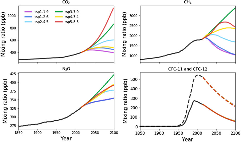
FIGURE 1. Evolution of CO₂, CH₄, N₂O, CFC-11 and CFC-12 surface mixing ratios throughout the historical period (1850–2014; black) and projected into the future under the Shared Socioeconomic Pathways (2014–2100; colored lines). For the CFC panel, CFC-11 is shown in the solid lines and CFC-12 in the dashed lines.

For each of the ML models explored here, annual mean surface mixing ratios of CO₂, CH₄, N₂O, CFC-11 and CFC-12 are used as input features for the machine learning algorithm, while the target feature is the annual mean stratospheric column ozone, averaged from 30°S–30°N. The stratospheric column ozone used in this study is smoothed using an 11-point boxcar smoothing to reduce both the effects of short-term variability and the signature of the 11 years solar cycle. In contrast, the emissions of CO₂, CH₄, N₂O, CFC-11 and CFC-12 already follow very smooth trajectories, and so these input features are not smoothed in the same way. In order to build the ML models, the data must be split into training and testing sets. For this work, each of the 4 ML methods investigated here was trained on UKESM1 output from the Historical and five of the SSP scenarios and then tested on the sixth (i.e., to make predictions of stratospheric column ozone changes under the SSP3-7.0 scenario, the machine learning was trained using output from the Historical, SSP1-1.9, SSP1-2.6, SSP2-4.5, SSP4-6.4 and SSP5-8.5 scenarios). For the Ridge and Lasso regression methods the input features of both the training and test data were scaled to a mean of zero and a standard deviation of one prior to the regression, while the Random Forest and Extra Trees methods use the unmodified datasets. The hyperparameters (e.g., the number of trees, whether bootstrapping is used, the maximum number of features selected, etc) of the machine learning algorithms are tuned using a 6-fold cross validation on the training data.

Results

UKESM1 projections of tropical stratospheric column ozone under the different SSP scenarios, smoothed using an 11-point boxcar smoothing, are shown in Figure 2. There is little difference between the projections in the first half of the 21st century, with reductions in stratospheric chlorine loadings resulting in positive trends in stratospheric column ozone, which increases from 258.5 DU in 2014 to 260.5 DU in 2050. In contrast, the scenarios diverge significantly in the latter half of the 21st century. Under SSP1-1.9 and SSP1-2.6 stratospheric column ozone continues to increase linearly between 2050 and 2100, reaching 264 DU by the end of the century, while for the same period stratospheric column ozone remains relatively constant under SSP2-4.5, SSP3-7.0 and SSP4-3.4. The most notable difference occurs under SSP5-8.5, in which stratospheric column ozone remains constant from 2050–2070, before decreasing from 2070–2100. In this scenario, stratospheric column ozone in the year 2100 is projected to be as low as it was in 2014, indicating that the impacts of anthropogenic emissions of greenhouse gases can entirely offset projected increases in stratospheric column ozone driven by reductions in hODSs. Stratospheric column ozone does not return to the 1980 (266 DU) or 1960 (270 DU) values modeled in the historical simulation under any SSP scenario.

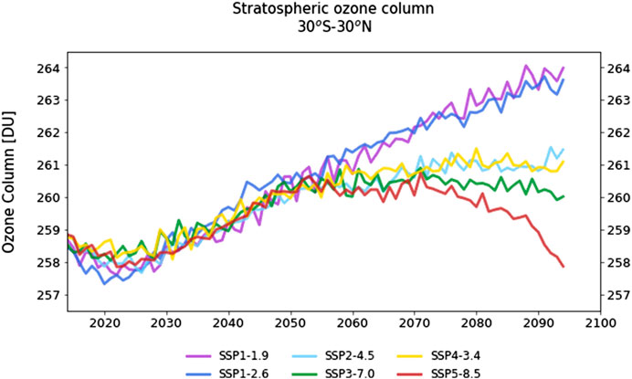
FIGURE 2. UKESM1 projections of stratospheric column ozone under different Shared Socioeconomic Pathways, averaged over 30°S–30°N. Projections shown here have been smoothed using an 11-point boxcar smoothing applied to the annual mean stratospheric column ozone values.

Figure 3 shows the percentage difference in zonal mean stratospheric ozone mixing ratios between the end of century (2085–2100) and present day (2000–2015) for each SSP scenario. Broadly the change in ozone mixing ratios is similar across the scenarios; all show decreased mixing ratios in the tropical lower stratosphere by the end of the century and increased ozone mixing ratios in the polar lower stratosphere and at all latitudes above 35 km. Projected changes in polar lower stratosphere ozone are broadly similar in magnitude between the scenarios, with ozone increases largest in the southern hemisphere polar lower stratosphere, consistent with healing of the Antarctic ozone hole as stratospheric chlorine mixing ratios decline. In contrast, larger relative differences are modeled in the upper stratospheric and tropical lower stratospheric responses. Under SSP scenarios which assume small future changes in radiative forcing (e.g., SSP1-1.9 and SSP1-2.6), upper stratospheric ozone is projected to increase by 10–15%, while under SSP scenarios which assume larger future changes in radiative forcing (e.g., SSP3-7.0 and SSP5-8.5), upper stratospheric ozone is projected to increase by 25–30%. Differences are between the SSP scenarios are also modeled in the tropical lower stratosphere, where under SSP1-1.9 and SSP1-2.6 ozone mixing ratios are projected to remain close their present-day values, while under SSP3-7.0 and SSP5-8.5 ozone mixing ratios are projected to decrease by 40–50%. Larger decreases in lower stratospheric ozone mixing ratios are modeled under scenarios with higher assumed radiative forcing changes. These changes are consistent with other studies (e.g., Oman et al., 2010; Eyring et al., 2013; Meul et al., 2014; Banerjee et al., 2016; Keeble et al., 2017; Keeble et al., 2020), and the drivers of these changes are now well understood. In the tropical upper stratosphere, where the chemical lifetime of ozone is short (∼1 day), increases are driven by both a reduced stratospheric chlorine loading and cooling of the upper stratosphere through longwave emission by CO₂ (Fels et al., 1980), which in turn slows the rate of catalytic ozone destruction reactions (e.g., Haigh and Pyle, 1982; Jonsson et al., 2004). In the tropical lower stratosphere, where the chemical lifetime of ozone is long (∼1 month), decreases are driven by both a faster BDC, which transports ozone poor air into the tropical lower stratosphere, and reduced chemical ozone production due to the thicker overhead ozone column (e.g., Meul et al., 2014; Keeble et al., 2017).

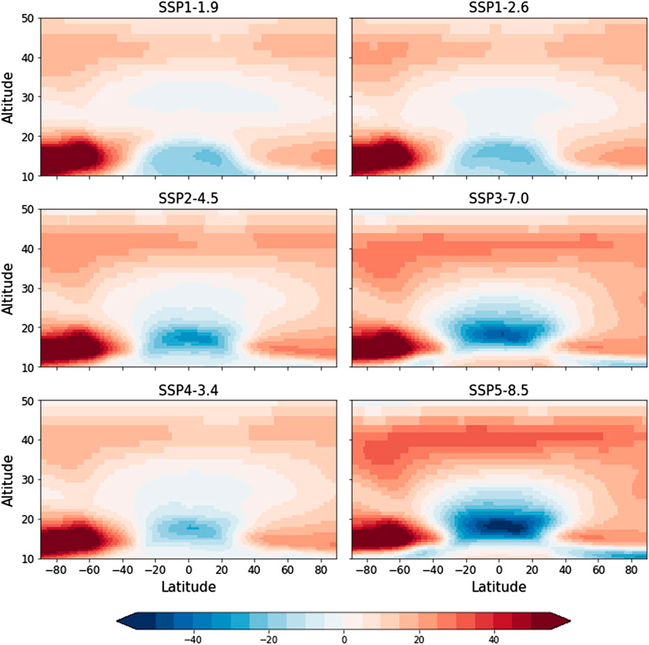
FIGURE 3. Percentage zonal mean ozone difference between the present day (2000–2014 averaged) and end of century (2086–2100 averaged) modeled by UKESM1 under the different Shared Socioeconomic Pathways.

The analysis presented above confirms that the UKESM1 model is making projections of tropical stratospheric column ozone which are consistent with current understanding of the drivers of future ozone changes. Distinct differences are modeled between the SSP scenarios in the evolution of stratospheric column ozone over the course of the 21st century, and it is hoped that suitably trained models built using machine learning techniques can accurately reproduce these differences. Projections of stratospheric ozone made using UKESM1 and four different machine learning techniques are shown in Figure 4. While differences are evident between the machine learning methods, all methods make reasonable projections, often falling within the range of UKESM1 ensemble members. Both Random Forests and Extra Trees (the non-linear methods) perform particularly well for SSP2-4.5, SSP3-7.0 and SSP4-3.4 predictions, with Extra Trees also making accurate predictions for SSP1-2.6. In contrast, there are periods of several decades in which the non-linear methods exceed the range of the UKESM1 ensemble for SSP1-1.9, and while both methods accurately predict the evolution of stratospheric column ozone under SSP5-8.5 between 2014–2070, neither captures the decrease in stratospheric column ozone modeled in the last few decades of the 21st century. This is perhaps not surprising, as the SSP5-8.5 scenario assumes CO₂ emissions much higher than in the other scenarios (Figure 1) and therefore, given the take-one-out method used to train the ML model, predictions in the last decades of the 21st century are being made well outside of the training data. In contrast, Ridge regression and Lasso regression) the linear methods) each perform well for SSP1-1.9, SSP1-2.6 and SSP2-4.5, but perform less well for SSP3-7.0, SSP4-3.4 and SSP5-8.5. Overall, when trained on the maximum amount of available data (i.e., the Historical simulation and all SSPs other than the one being predicted) there is no clearly better method from the four machine learning models tested here, and this is supported by root mean square errors (RMSE) calculated between the UKESM1 ensemble means and predicted stratospheric column ozone values for the various SSPs (Table 1).

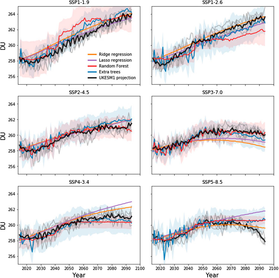
FIGURE 4. UKESM1 projections of stratospheric column ozone under different Shared Socioeconomic Pathways, averaged over 30°S–30°N, for the ensemble mean (black) and individual ensemble members (gray), smoothed using an 11-point boxcar smoothing. Also shown are predictions of stratospheric column ozone made using the four machine learning methods assessed in this study (Ridge regression, Lasso regression, Random Forests, Extra Trees). Envelops around the projections made using the Random Forest and Extra Trees methods represent 1σ uncertainty estimates in those projections, calculated using the infinitesimal jackknife method (Wager et al., 2014).

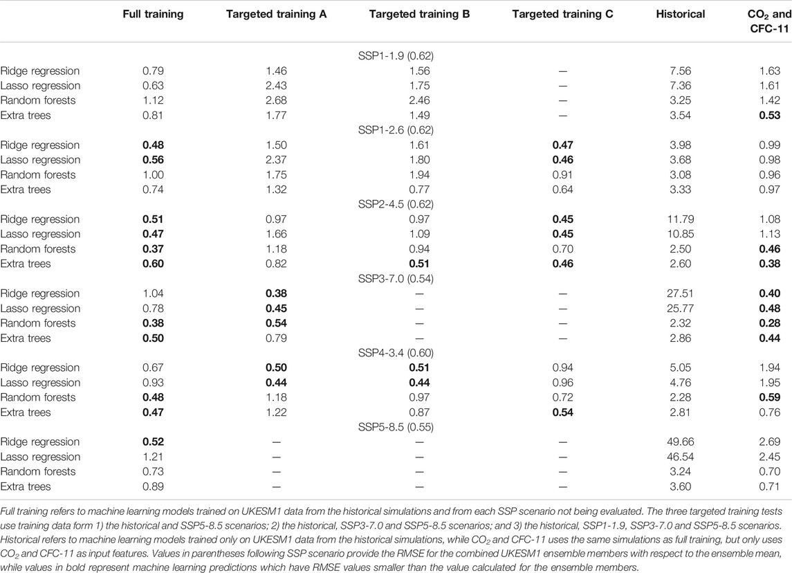
TABLE 1. Root mean square error (RMSE) for projections made using the four different machine learning methods, compared to the UKESM1 ensemble mean for each SSP scenario for different training conditions.

The ability for the methods to make accurate projections is predicated on being suitably trained. In the discussion above the most ideal case, training the machine learning models using UKESM1 data from every scenario except the one being predicted has been explored. In order to test the extent to which ML methods can make accurate projections when only weakly trained, the impacts of using different input features and numbers of scenarios has also been explored. In the first of these tests, the machine learning models were trained using smaller subsets of the UKESM1 simulations. These included training on UKESM1 data from the historical and SSP5-8.5 scenarios; the historical, SSP3-7.0 and SSP5-8.5 scenarios; and the historical, SSP1-1.9, SSP3-7.0 and SSP5-8.5 scenarios. The rationale behind these runs are as follows: together the historical, SSP1-1.9, SSP3-7.0 and SSP5-8.5 scenarios cover the extreme (highest and lowest) values for all five input features, while the historical and SSP5-8.5 together cover the extreme values for CO₂. For each of these tests, while machine learning predictions for individual scenarios can fall within the ensemble spread and have RMSE values smaller than the value calculated for the ensemble members (Table 1), performance is generally worse than for the full training case. A further test was performed in which the machine learning models were trained only on data from the UKESM1 historical simulations. In this case, no model is able to make accurate predictions for future SSP scenarios, and by the end of the 21st century the ML model predictions can differ from the UKESM1 results by more than 100 DU. This is due to the models being asked to make predictions with input features that are outside of the training dataset, and so rely on extrapolation, which can lead to large errors in prediction, especially for non-linear methods such as Random Forest and Extra Trees. A final test was performed in which the machine learning models were only trained using the same simulations as for the full training case but using only CO₂ and CFC-11 as input features (i.e., excluding N₂O, CH₄ and CFC-12). Under these conditions, performance of Random Forests and Extra Trees predictions is similar to the full training case, while the linear methods, Ridge and Lasso regression, perform noticeably worse for many of the SSPs. Predictions made using the Extra Trees method for each of these tests are shown in Figure 5, highlighting the difference in performance for predictions made using machine learning data when given different amounts of training data.

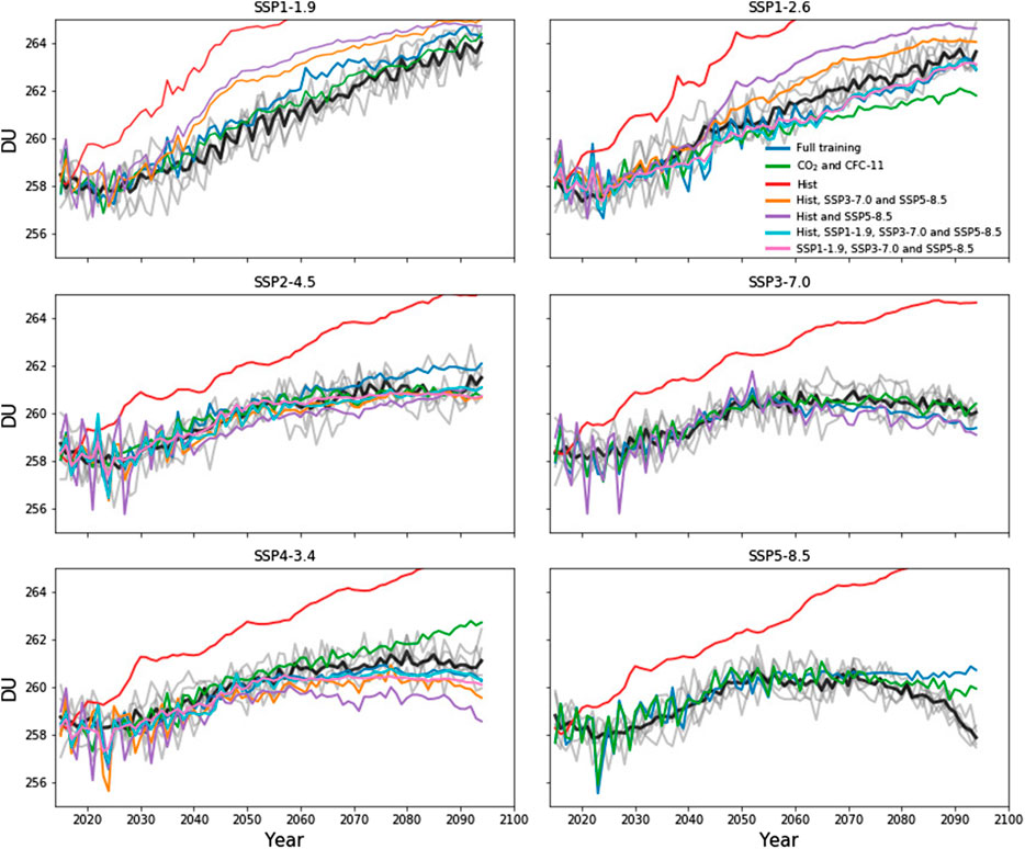
FIGURE 5. Predictions of tropical stratospheric column ozone made using the Extra Trees machine learning method using different amounts of training data.

Discussion and Conclusion

Results presented in this study highlight, for the first time, the potential for using machine learning techniques to make accurate, computationally inexpensive projections of tropical stratospheric column ozone for a range of different future emissions scenarios. Four machine learning techniques were investigated, two linear techniques (Ridge and Lasso regression) and two non-linear techniques (Random Forests and Extra Trees), using CO₂, CH₄, N₂O, CFC-11 and CFC-12 surface mixing ratios as input features. When trained on data from an ensemble of historical simulations and five of the six available SSP scenarios performed by the UKESM1 Earth system model, the machine learning techniques investigated here are able to accurately predict the evolution of tropical stratospheric column ozone over the course of the 21st century for a large number of the different SSP scenarios. However, all machine learning approaches struggle to make accurate predictions of the SSP5-8.5 scenario during the last few decades of the 21st century when trained on the historical simulation and the other SSP scenarios. During these decades, stratospheric column ozone begins to decline, driven by an increase in the speed of the BDC. However, this occurs under CO₂ mixing ratios which are outside of the range seen in the training datasets (i.e., the other model scenarios), and this highlights the difficulty encountered by machine learning techniques in making accurate predications when required to extrapolate beyond the range of training data. Despite this, machine learning techniques can make accurate predictions of the more moderate future emissions scenarios and show great promise in being able to supplement future scenarios modeled by fully coupled chemistry-climate and Earth system models.

A key requirement for making accurate predictions with machine learning methods is providing sufficient training datasets, and the amount of data required to make accurate predictions was explored in this study. While none of the methods explored here were able to make accurate predictions of the future evolution of stratospheric column ozone when only provided with data from historical simulations for training, several methods show greater promise when trained on selected scenarios. The Extra Trees method was shown to make accurate predictions of stratospheric column ozone, falling within the ensemble spread from the UKESM1 projections, for the SSP1-2.6, SSP2-4.5 and SSP4-3.4 when trained on data from the historical simulations and SSP1-1.9, SSP3-7.0 and SSP5-8.5 scenarios, and also make accurate projections when trained only the historical simulations and SSP5-8.5 scenarios for some scenarios.

The machine learning models explored in this study were built using only information about the surface concentration (and by extension emissions) of key anthropogenic species as input features. This methodology has the benefit of using input features that can be directly controlled by policy decisions, and the result is that these models would provide an estimate of the future evolution of tropical stratospheric column ozone for any combination of CO₂, CH₄, N₂O, CFC-11 and CFC-12 surface mixing ratios which fell within the range of the training data (i.e., the SSPs explored in this study). A limitation however is that the machine learning models are not confronted with any process-based information during the training process. Examples of these process-based input features include age-of-air tracers and/or ${\overline{w}}^{\ast }$to provide a measure of the speed of the BDC, and reaction flux diagnostics to provide a measure of the chemical depletion of ozone. By choosing different input features to those used in this study it may be possible to produce more accurate projections of tropical stratospheric ozone. However, in order to include these features in machine learning models some understanding of how they will evolve in the future would be required, necessitating simulations performed with chemistry-climate or Earth system models. The work presented here provides a first exploration of the use of relatively simple machine learning models for making projections of stratospheric ozone, and there remains work to do in selecting the best combination of input features and identifying whether more complex machine learning approaches, such as neural networks, can be used to further improve upon the models explored in this study.

It will always be necessary to make projections of future changes to atmospheric composition with coupled chemistry-climate and Earth system models. Additionally, it is important to bear in mind that chemistry-climate and Earth system models can provide much wider output, spanning a huge range of important chemistry and climate variables, than is provided by models of just stratospheric column ozone. However, the work performed here indicates that machine learning and statistical models can be used to reduce the computational burden required by performing large numbers of future scenarios for studies which wish to know how stratospheric column ozone may respond to future emissions changes. Results presented here indicate that if Earth system models and/or chemistry climate models simulations are run following scenarios with the largest and smallest estimates of future greenhouse gas emissions (i.e., SSP1-1.9, SSP3-7.0 and SSP5-8.5), machine learning approaches could be used to provide estimates of stratospheric ozone evolution under the “middle-of-the-road” scenarios (e.g., SSP2-4.5, SSP4-3.4). In the future, it is hoped to expand the training of the machine learning models explored here to use ozone from all CMIP6 models. Additionally, it remains to be tested whether these models can accurately predict the evolution of stratospheric ozone in other latitudinal ranges. Finally, it is hoped that the models investigated here can be expanded to provide vertically resolved ozone changes, which would provide an important step toward using machine learning based models within climate models which do not have interactive chemistry schemes to estimate stratospheric ozone changes.

Data Availability Statement

The datasets presented in this study can be found in online repositories. The names of the repository/repositories and accession number(s) can be found below: The UKESM1 datasets used in this study are available through the Earth System Grid Federation (ESGF; https://esgf-index1.ceda.ac.uk/projects/cmip6-ceda/). A GUI which enables readers to run all of the methods used in this study themselves can be found at www.scottyiu.com, while files containing the input features and training data are included with this article in the Supplementary Material.

Author Contributions

JK and YYSY developed the machine learning based models explored in the manuscript. JK, AA, FO’C, AS, and JW contributed toward development of the UKESM1 model. All authors contributed to the preparation of the manuscript.

Conflict of Interest

The authors declare that the research was conducted in the absence of any commercial or financial relationships that could be construed as a potential conflict of interest.

The reviewer AF declared a past co-authorship with several of the authors AA, FOC to the handling editor.

Acknowledgments

JK, AA, and JP thank NERC for financial support through NCAS (Funder reference: R8/H12/83/003). We acknowledge use of the Monsoon2 system, a collaborative facility supplied under the Joint Weather and Climate Research Program, a strategic partnership between the Met Office and the Natural Environment Research Council. We acknowledge the World Climate Research Program, which, through its Working Group on Coupled Modeling, coordinated and promoted CMIP6, and the multiple funding agencies who support CMIP6 and ESGF.

Supplementary Material

The Supplementary Material for this article can be found online at: https://www.frontiersin.org/articles/10.3389/feart.2020.592667/full#supplementary-material.

References

Archibald, A. T., O'Connor, F. M., Abraham, N. L., Archer-Nicholls, S., Chipperfield, M. P., Dalvi, M., et al. (2020). Description and evaluation of the UKCA stratosphere-troposphere chemistry scheme (StratTrop vn 1.0) implemented in UKESM1. Geosci. Model Dev. 13, 1223–1266. doi:10.5194/gmd-13-1223-2020
Austin, J., Hood, L. L., and Soukharev, B. E. (2017). Solar cycle variations of stratospheric ozone and temperature in simulations of a coupled chemistry-climate model. Atmos. Chem. Phys. 7, 1693–1706. doi:10.5194/acp-7-1693-2007
Balaji, V., Taylor, K. E., Juckes, M., Lawrence, B. N., Durack, P. J., Lautenschlager, M., et al. (2018). Requirements for a global data infrastructure in support of CMIP6. Geosci. Model Dev. 11, 3659–3680. doi:10.5194/gmd-11-3659-2018
Bernhard, G. H., Neale, R. E., Barnes, P. W., Neale, P. J., Zepp, R. G., Wilson, S. R., et al. (2020). Environmental effects of stratospheric ozone depletion, UV radiation and interactions with climate change: UNEP Environmental Effects Assessment Panel, update 2019. Photochem. Photobiol. Sci. 19, 542–584. doi:10.1039/d0pp90011g
Brewer, A. W. (1949). Evidence for a world circulation provided by the measurements of helium and water vapour distribution in the stratosphere. Q.J Royal Met. Soc. 75 (326), 351–363. doi:10.1002/qj.49707532603
Dhomse, S. S., Kinnison, D., Chipperfield, M. P., Salawitch, R. J., Cionni, I., Hegglin, M. I., et al. (2018). Estimates of ozone return dates from Chemistry-Climate Model Initiative simulations. Atmos. Chem. Phys. 18, 8409–8438. doi:10.5194/acp-18-8409-2018
Dobson, G. M. B. (1956). Origin and distribution of the polyatomic molecules in the atmosphere. Proc. Roy. Soc. Lond. Math. Phys. Sci. 236 (1205), 187–193. doi:10.1098/rspa.1956.0127
Eyring, V., Arblaster, J. M., Cionni, I., Sedláček, J., Perlwitz, J., Young, P. J., et al. (2013). Long-term ozone changes and associated climate impacts in CMIP5 simulations. J. Geophys. Res. Atmos. 118, 5029–5060. doi:10.1002/jgrd.50316
Eyring, V., Bony, S., Meehl, G. A., Senior, C. A., Stevens, B., Stouffer, R. J., et al. (2016). Overview of the coupled model intercomparison project phase 6 (CMIP6) experimental design and organization. Geosci. Model Dev. 9, 1937–1958. doi:10.5194/gmd-9-1937-2016
Geurts, P., Ernst, D., and Wehenkel, L. (2006). Extremely randomized trees. Mach. Learn. 63, 3–42. doi:10.1007/s10994-006-6226-1
Good, P., Sellar, A., Tang, Y., Rumbold, S., Ellis, R., Kelley, D., et al. (2019). MOHC UKESM1.0‐LL model output prepared for CMIP6 ScenarioMIP. Earth System Grid Federation. Available at: doi.org/10.22033/ESGF/CMIP6.1567.Version.20191101
Guilyardi, A., Maycock, A. C., Archibald, A. T., Abraham, N. L., Telford, P., Braesicke, P., et al. (2016). Drivers of changes in stratospheric and tropospheric ozone between year 2000 and 2100. Atmos. Chem. Phys. 16, 2727–2746. doi:10.5194/acp-16-2727-2016
Haigh, J. D., and Pyle, J. A. (1982). Ozone perturbation experiments in a two-dimensional circulation model. Q.J Royal Met. Soc. 108, 551–574. doi:10.1002/qj.49710845705
Hoerl, A. E., and Kennard, R. W. (1970). Ridge regression: biased estimation for nonorthogonal problems. Technometrics 12 (1), 55–67. doi:10.1080/00401706.1970.10488634
Jonsson, A. I., De Grandpre, J., Fomichev, V. I., McConnell, J. C., and Beagley, S. R. (2004). Doubled CO2-induced cooling in the middle atmosphere: Photochemical analysis of the ozone radiative feedback. J. Geophys. Res. 109, D24103. doi:10.1029/2004jd005093
Keeble, J., Bednarz, E. M., Banerjee, A., Abraham, N. L., Harris, N. R. P., Maycock, A. C., and Pyle, J. A. (2017). Diagnosing the radiative and chemical contributions to future changes in tropical column ozone with the UM-UKCA chemistry-climate model. Atmos. Chem. Phys. 17, 13801–13818. doi:10.5194/acp-17-13801-2017
Keeble, J., Hassler, B., Banerjee, A., Checa-Garcia, R., Chiodo, G., Davis, S., et al. (2020). Evaluating stratospheric ozone and water vapor changes in CMIP6 models from 1850-2100. Atmos. Chem. Phys. Discuss. doi:10.5194/acp-2019-1202
Meinshausen, M., Nicholls, Z. R. J., Lewis, J., Gidden, M. J., Vogel, E., Freund, M., et al. (2020). The shared socio-economic pathway (SSP) greenhouse gas concentrations and their extensions to 2500. Geosci. Model Dev. 13, 3571–3605. doi:10.5194/gmd-13-3571-2020
Meul, S., Dameris, M., Langematz, U., Abalichin, J., Kerschbaumer, A., Kubin, A., et al. (2016). Impact of rising greenhouse gas concentrations on future tropical ozone and UV exposure. Geophys. Res. Lett. 43, 2919–2927. doi:10.1002/2016gl067997
Meul, S., Langematz, U., Oberländer, S., Garny, H., and Jöckel, P. (2014). Chemical contribution to future tropical ozone change in the lower stratosphere. Atmos. Chem. Phys. 14, 2959–2971. doi:10.5194/acp-14-2959-2014
Nowack, P., Braesicke, P., Haigh, J., Abraham, N. L., Pyle, J., and Voulgarakis, A. (2018). Using machine learning to build temperature-based ozone parameterizations for climate sensitivity simulations. Environ. Res. Lett. 13 (10), 104016. doi:10.1088/1748-9326/aae2be
O’Neill, B. C., Tebaldi, C., Van Vuuren, D. P., Eyring, V., Friedlingstein, P., Hurtt, G., et al. (2016). The scenario model intercomparison project (ScenarioMIP) for CMIP6. Geosci. Model Dev. (GMD) 9, 3461–3482. doi:10.5194/gmd-9-3461-2016
Oman, L. D., Plummer, D. A., Waugh, D. W., Austin, J., Scinocca, J. F., Douglass, A. R., et al. (2010). Multimodel assessment of the factors driving stratospheric ozone evolution over the 21st century. J. Geophys. Res. 115, D24306. doi:10.1029/2010jd014362
Phillips, D. L. (1962). A technique for the numerical solution of certain integral equations of the first kind. J. ACM 9, 84–97. doi:10.1145/321105.321114
Riahi, K., Van Vuuren, D. P., Kriegler, E., Edmonds, J., O’Neill, B. C., Fujimori, S., et al. (2017). The shared socioeconomic pathways and their energy, land use, and greenhouse gas emissions implications: an overview. Global Environ. Change 42, 153–168. doi:10.1016/j.gloenvcha.2016.05.009
Sellar, A. A., Jones, C. G., Mulcahy, J. P., Tang, Y., Yool, A., Wiltshire, A., et al. (2019). UKESM1: description and evaluation of the U.K. Earth system model. J. Adv. Model. Earth Syst. 11 (12), 4513–4558. doi:10.1029/2019ms001739
Solomon, S. (1999). Stratospheric ozone depletion: a review of concepts and history. Rev. Geophys. 37, 275–316. doi:10.1029/1999RG900008
Son, S.-W., Gerber, E. P., Perlwitz, J., Polvani, L. M., Gillett, N. P., Seo, K.-H., et al. (2010). Impact of stratospheric ozone on Southern Hemisphere circulation change: a multimodel assessment. J. Geophys. Res. 115, D00M07. doi:10.1029/2010jd014271
Tang, Y., Rumbold, S., Ellis, R., Kelley, D., Mulcahy, J., Sellar, A., et al. (2019). MOHC UKESM1.0-LL model output prepared for CMIP6 CMIP historicalEarth System Grid Federation. doi:10.22033/ESGF/CMIP6.6113.Version.20191101
Thompson, D. W. J., Solomon, S., Kushner, P. J., England, M. H., Grise, K. M., and Karoly, D. J. (2011). Signatures of the Antarctic ozone hole in Southern Hemisphere surface climate change. Nat. Geosci. 4, 741–749. doi:10.1038/ngeo1296
Thompson, D. W. J., and Solomon, S. (2009). Understanding recent stratospheric climate change. J. Clim. 22 (8), 1934–1943. doi:10.1175/2008jcli2482.1
Tibshirani, R. (1996). A comparison of some error estimates for neural network models. Neural Comput. 8 (1), 152–163. doi:10.1162/neco.1996.8.1.152
Wager, S, Hastie, T, and Efron, B (2014). Confidence intervals for random forests: the jackknife and the infinitesimal jackknife. J. Mach. Learn. Res. 15 (1), 1625–1651.
Weber, M., Coldewey-Egbers, M., Fioletov, V. E., Frith, S. M., Wild, J. D., Burrows, J. P., et al. (2018). Total ozone trends from 1979 to 2016 derived from five merged observational datasets - the emergence into ozone recovery. Atmos. Chem. Phys. 18, 2097–2117. doi:10.5194/acp-18-2097-2018
WMO (2018). “Scientific assessment of ozone depletion: 2018,” in Global ozone research and monitoring project—report No., 58. Geneva, Switzerland: WMO (World Meteorological Organization), 588.
Keywords: machine learning, earth system model, stratospheric ozone, future ozone projections, UKESM1, CMIP6
Citation: Keeble J, Yiu YYS, Archibald AT, O’Connor F, Sellar A, Walton J and Pyle JA (2021) Using Machine Learning to Make Computationally Inexpensive Projections of 21st Century Stratospheric Column Ozone Changes in the Tropics. Front. Earth Sci. 8:592667. doi: 10.3389/feart.2020.592667
Received: 07 August 2020; Accepted: 09 November 2020;
Published: 14 January 2021.
Edited by:
Timofei Sukhodolov, Physikalisch-Meteorologisches Observatorium Davos, SwitzerlandReviewed by:
Aryeh Feinberg, ETH Zurich, SwitzerlandMartin Schultz, Jülich Supercomputing Centre, Forschungszentrum Jülich, Germany
Copyright © 2021 Keeble, Yiu, Archibald, O'connor, Sellar, Walton and Pyle. This is an open-access article distributed under the terms of the Creative Commons Attribution License (CC BY). The use, distribution or reproduction in other forums is permitted, provided the original author(s) and the copyright owner(s) are credited and that the original publication in this journal is cited, in accordance with accepted academic practice. No use, distribution or reproduction is permitted which does not comply with these terms.
*Correspondence: James Keeble, james.keeble@atm.ch.cam.ac.uk