Quantifying uncertainty of machine learning methods for loss given default

1. Introduction

Financial institutions play a central role in the stability of the financial sector. They act as intermediaries to support the supply of money and lending as well as the transfer of risk between entities. However, this exposes financial institutions to several types of risk, including credit risk. Credit risk has the largest stake with roughly 84% of risk-weighted assets of 131 major EU banks as of June 2021 [1]. The expected loss (EL) due to credit risk is composed of three parameters: Probability of Default (PD), Loss Given Default (LGD), and Exposure at Default (EAD). PD is defined as the probability that a creditor will not comply with his agreed obligations at a later time. LGD is defined as the relative fraction of the outstanding amount that is lost. Finally, EAD is defined as the outstanding amount at the time of default.

This article focuses on LGD as this risk parameter is important for financial institutions not only from a risk management perspective but also for pricing credit risky assets. Financial institutions can use their own models to calculate an estimate for the LGD. This estimate is subsequently used to determine the interest on the loan/bond and the capital requirement for the financial institution itself see, e.g., [2–6]. Depending on the defaulted asset, we can divide the LGD further into market-based and workout LGD. The former refers to publicly traded instruments like bonds and is commonly defined as one minus the ratio of the market price 30 days after default divided by the outstanding amount at the time of default. The latter refers to bank loans and is determined by accumulating discounted payments from creditors during the default resolution process. In this article, we use a record of nearly three decades of market-based LGDs gathered from the Moody's Default and Recovery Database starting in January 1990 until December 2019. Recent literature using a shorter history of this data documents that machine learning models due to their ability to account for non-linear relationships of drivers and LGD estimates outperform standard statistical methods, see, e.g., [7–9]. Fraisse and Laporte [10] show that allowing for non-linearity can be beneficial in many risk management applications and can lead to a better estimation of the capital requirements for banks. Therefore, using machine learning models can increase the precision of central credit risk parameters and, as a consequence, could have the potential to yield more adequate capital requirements for banks due to the increased precision.

There is a large body of literature using advanced statistical methods for LGDs. These include beta regression, factorial response models, local logit regressions, mixture regression, and quantile regression among many others, see, e.g., [2–4, 9, 11–18]. Concerning the increased computational power and methodical progress in academia, machine learning models have become more and more frequently applied concerning LGDs¹. Early studies by Matuszyk et al. [28] and Bastos [12] employ tree-based methods. Moreover, several studies provide benchmark exercises using various machine learning methods, see, e.g., [13–15]. Bellotti et al. [5] and Kaposty et al. [29] update previous benchmark studies with new data and algorithms. Nazemi et al. [30] find text-based variables to be important drivers for marked-based LGDs. Furthermore, evidence that spatial dependence plays a key role in peer-to-peer lending LGD estimation can be found in Calabrese and Zanin [31]. By combining statistical and machine learning models, Sigrist and Hirnschall [32] and Kellner et al. [6] show that benefits from both worlds can be captured.

An important aspect, to which the machine learning LGD literature has not yet paid attention, is the associated uncertainty around estimates and predictions². Commonly, we can define two types of uncertainty, aleatoric and epistemic [33]. Following Gawlikowski et al. [34], aleatoric uncertainty is the uncertainty in the data itself that can not be reduced and is therefore also known as irreducible or data uncertainty. In classical statistics, this type of uncertainty is for example represented by ϵ in the linear regression framework. Epistemic uncertainty refers to the uncertainty of a model due to the (limited) sample size. This uncertainty can be reduced by increasing the sample size on which the model is trained and is therefore also known as reducible or model uncertainty [34]. In a linear regression setting, epistemic uncertainty is, accounted for by the standard errors of the beta coefficients. Given a larger sample size, the standard errors should decrease. Recently, the literature on uncertainty estimation has grown rapidly as outlined in a survey article by Gawlikowski et al. [34].

A first intuitive way to quantify uncertainty is the Bayesian approach, which is also common in classical statistics. However, Bayesian neural networks are computationally expensive and do not scale easily to complex neural network architectures containing many parameters. Therefore, other researchers aim at approximating Bayesian inference/prediction for neural networks. Blundell et al. [35] introduce a backpropagation-compatible algorithm to learn probability distributions of weights instead of only point estimates. They call their approach “Bayes by Backprop.” Rather than apply Bayesian principles at the time of training, another strand of literature tries to approximate the posterior distribution only at the time of prediction. Gal and Ghahramani [36] introduce a concept called Monte Carlo Dropout, which applies a random dropout layer at the time of prediction to estimate uncertainty. Another variant of this framework is called Monte Carlo DropConnect by Mobiny et al. [37]. This variant uses the generalization of Dropout Layers, called DropConnect Layers, where the dropping is applied directly to each weight, rather than to each output unit. The DropConnect approach has outperformed Dropout in many applications and data sets, see, e.g., [37]. Another strategy is to use so-called hypernetworks [38]. This type of network is a neural network that produces parameters of another neural network (so-called primary network) with random noise input. Finally, the hyper and primary neural networks together form a single model that can easily be trained by backpropagation. Another strand of literature applies an ensemble of methods and uses their information to approximate uncertainty, see, e.g., [39–41]. However, these approaches are computationally more expensive than Dropout or DropConnect-related approaches. A further strand of literature aims at predicting the types of uncertainty directly within the neural network structure. One of these approaches is called deep evidential regression by Amini et al. [42] and extensions by Meinert et al. [43], which learn the parameters of a so-called evidential distribution. This method quantifies uncertainty without extra computations after training. Additionally, the estimated parameters of the evidential distribution can be plugged into analytical formulas for epistemic and aleatoric uncertainty. This approach quantifies uncertainty in a fast and traceable way without any additional computational burden. Because it has many advantages, this article relies on the deep evidential regression framework.

We contribute to the literature in two important ways. First, this article applies an uncertainty estimation framework in machine learning LGD estimation and prediction. We observe that deep evidential regression provides a sound and fast framework to quantify both, aleatoric and epistemic uncertainty. This is important with respect to regulatory concerns. Not only is explainability required by regulators, the quantification of uncertainty surrounding their predictions may be a fruitful step toward the acceptance of machine learning algorithms in regulatory contexts. Second, this article analyzes the ratio between aleatoric and epistemic uncertainty and finds that aleatoric uncertainty is much larger than epistemic uncertainty. This implies that the largest share of uncertainty comes from the data itself and, thus, cannot be reduced. Epistemic uncertainty, i.e., model uncertainty, plays only a minor role. This may explain why advanced methods may outperform simpler ones, but still, the estimation and prediction of LGD remain a very challenging task.

The remainder of this article is structured as follows. Data is presented in Section 2, while the methodology is described in Section 3. Our empirical results are discussed in Sections 4, 5 concludes.

2. Data

To analyze bond loss given defaults, we use Moody's Default and Recovery Database (Moody's DRD). This data has information regarding the market-based LGD, default type, and various other characteristics of 1,999 US bonds from January 1990 until December 2019³. We use bond characteristics such as the coupon rate, the maturity, the seniority of the bond, and an additional variable, which indicates whether the bond is backed by guarantees beyond the bond issuer's assets. Furthermore, we include a binary variable, which determines if the issuer's industrial sector belongs to the FIRE (finance, insurance, or real estate) sector. To control for differences due to the reason of default, we also include the default type in our analysis. In addition to that, we add the S&P 500 return to control for the macroeconomic surrounding. Consistent with Gambetti et al. [4], we calculate the US default rates directly from Moody's DRD. To control for withdrawal effects, we use the number of defaults occurring in a given month divided by the number of firms followed in the same period. Since we are interested in the uncertainty in the LGD estimation, we include uncertainty variables. To incorporate financial uncertainty, we use the financial uncertainty index by Jurado et al. [44] and Ludvigson et al. [45] which is publicly available on their website. Finally, we include the news-based economic policy uncertainty index provided by Baker et al. [46], which is also accessible on his website. To keep predictive properties, we lag all macroeconomic variables and uncertainty indices by one-quarter similar to Olson et al. [8].

Our dependent variable shows a mode at 90%, illustrated in Figure 1. This is consistent with Gambetti et al. [4], who analyzed the recovery rates. The average LGD is about 64.29% as shown in Table 1 with a standard deviation of 27.59%. The sample also covers nearly the whole range of market-based LGDs with a minimum of 0.5% and a maximum of 99.99%.

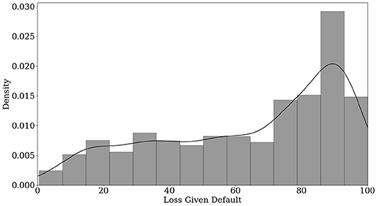
Figure 1. Histogram of LGDs.

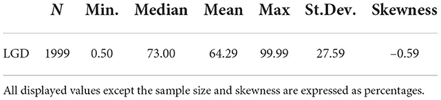
Table 1. Descriptive statistics of LGDs across the whole sample.

Table 2 lists the variables and data types. In total, we use six bond-related variables, two macroeconomic, and two uncertainty-related variables. The categorical bond-related variables act as control variables for differences in the bond structure.

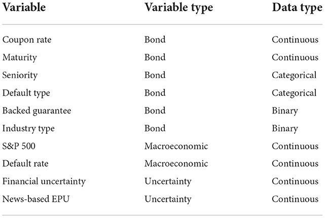
Table 2. Selected variables for the network.

Table 3 shows the correlations between macroeconomic and uncertainty variables. The correlation is moderate to strong across the variables. This must be taken into account when interpreting the effects of the variables. The only exception is the financial uncertainty index and the default rate, which have a very weak correlation.

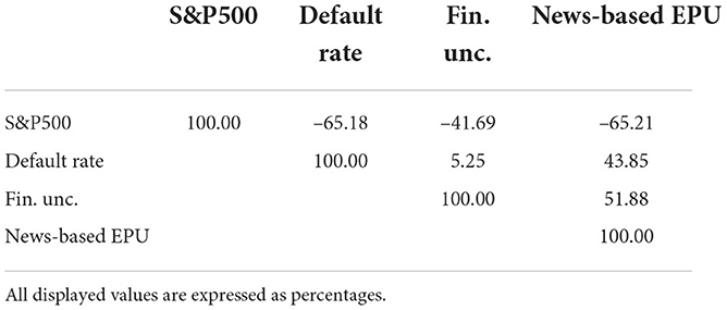
Table 3. Upper triangle of the correlation matrix of macroeconomic and uncertainty features.

Table 4 shows descriptive statistics for the seniority of the bond. Each subcategory captures the whole range of LGDs, while the mean and the median of Senior Secured bonds are comparably low. In addition, the Senior Secured bonds have almost no skewness, while the skewness of Senior Unsecured bonds is moderate. The skewness of Senior Subordinated and Subordinated bonds is more negative and fairly similar. Comparing the descriptive statistics across seniority, we observe that the locations of the distributions are different, but the variation of the distribution is considerably large. This might be the first indication of large (data) uncertainty.

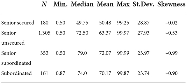
Table 4. Descriptive statistics of LGDs according to the seniority of the defaulted bond.

Table 5 categorizes the LGDs by their default type, which alters some aspects of the overall picture. Compared to Table 1, the categories Distressed Exchange and Others have lower mean and median LGD and positive skewness. The biggest difference between these two categories is that Distressed Exchange has a lower standard deviation. Missed Interest Payment and Prepackaged Chapter 11 show similar descriptive statistics compared to the whole sample in Table 1. The last category Chapter 11 has even higher mean and median LGD and the skewness is fairly low.

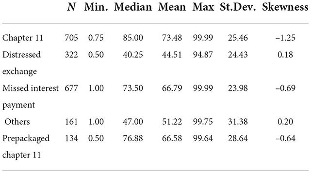
Table 5. Descriptive statistics of LGDs according to the default type.

3. Methods

To model the uncertainty of LGDs, we use a framework called deep evidential regression by Amini et al. [42]. This method is capable of determining the uncertainty of regression tasks and estimating the epistemic and the aleatoric uncertainty. One way to model aleatoric uncertainty in the regression case is to train a neural network with weights w based on the negative log-likelihood of the normal distribution, and thus perform a maximum likelihood optimization. The objective function for each observation is Amini et al. [42]:

Where y_i is the i-th LGD observation of the sample with size N and μ_i and ${\sigma }_i^2$ the mean and the variance of the assumed normal distribution for observation i. Since μ_i and ${\sigma }_i^2$ are unknown, they can be modeled in a probabilistic manner by assuming they follow prior distributions q(μ_i) and $q({\sigma }_i^2)$. Following Amini et al. [42], for μ_i a normal distribution and for ${\sigma }_i^2$ a inverse gamma distribution is chosen:

With γ_i ∈ ℝ, ν_i > 0, α_i > 1 and β_i > 0. Factorizing the joint prior distribution $q({\mu }_i,{\sigma }_i^2)=q({\mu }_i)q({\sigma }_i^2)$ results in a normal inverse gamma distribution:

This normal inverse gamma distribution can be viewed in terms of virtual observations, which can describe the total evidence Φ_i. Contrary to Amini et al. [42], we take the suggested definition of the total evidence in Meinert et al. [43] as Φ_i = ν_i + 2α_i, because as derived in Meinert et al. [47], the parameters ν_i and 2α_i of the conjugated prior normal inverse gamma distribution can be interpreted as virtual observations of the prior distribution, where μ_i and ${\sigma }_i^2$ are estimated from. As a result, the total evidence is the sum of those two expressions. By choosing the negative inverse gamma distribution as the prior distribution, there exists an analytical solution for computing the marginal likelihood or model evidence if the data follows a normal distribution [42, 43]. The marginal likelihood, therefore, follows a student-t distribution:

The marginal likelihood represents the likelihood of obtaining observation y_i given the parameter of the prior distribution, in this case, γ_i, ν_i, α_i, and β_i. Therefore, maximizing the marginal likelihood maximizes the model fit. This can be achieved by minimizing the negative log likelihood of p(y_i|γ_i, ν_i, α_i, β_i). Due to the special conjugated setting with normally distributed data and normal inverse prior distributions, the marginal likelihood can be calculated in a closed form [42]:

Such that Ω_i = 2β_i(1 + ν_i) and Γ(.) represents the gamma function. This closed-form expression makes deep evidential regression networks fast to compute. To get an accurate estimate of the aleatoric and the epistemic uncertainty the loss function has to be regularized. Contrary to the original formulation of Amini et al. [42], Meinert et al. [43] suggest a different regularization term because when using the original formulation the regularized likelihood is insufficient to find the parameters of the marginal likelihood. Therefore, we follow the approach of Meinert et al. [43] and use the adjusted regularization term. This adjustment scales the residuals by the width of the student-t distribution in Eq. (5), w_Sti, such that the gradients of Φ_i and therefore, of ν_i do not tend to get very large in noisy regions:

With p being the strength of the residuals on the regularization. The loss function for the neural network can therefore be calculated as:

Where λ is a hyperparameter to determine the strength of the regularization in Eq. (7). Since λ and p have to be determined in advance the network has four output neurons, corresponding to each parameter of the marginal likelihood in Eq. (5). These parameters can be used to quantify uncertainty. Due to the close connection between the student-t and the normal distribution, w_Sti can be used as an approximation for the aleatoric uncertainty [43]. Following Meinert et al. [43], the epistemic and aleatoric uncertainty can be derived as follows:

By employing this approach, we assume that our dependent variable, y, follows a normal distribution. LGDs are commonly bound in the interval between zero to one, which is only a part of the space of the normal distribution. Hence, there is the possibility that we obtain predicted values outside this range. However, using the normality assumption is very common in LGD research as the OLS regression is frequently used as the main method or at least as a benchmark to other methods, see, e.g., [5, 11, 13–15, 17, 29, 48–53]. Anticipating the results in Section 4, we will see that the predicted values for almost all bonds lie in the interval between zero to one and, thus, our approach produces reasonable estimates. Furthermore, the deep evidential regression approach requires some assumptions to obtain a closed-form solution. For other distributional assumptions, e.g., a beta distribution for the LGD, there is no closed-form marginal likelihood known, which, if used, would eliminate the advantages of this approach.

To unveil the relationships modeled by the neural network, we use Accumulated Local Effect (ALE) plots by Apley and Zhu [54]. ALE plots visualize the average effect of the independent variables on the prediction. Another advantage of ALE plots over other explainable artificial intelligence (XAI) methods is that they are unbiased and fast to compute. As mentioned in Section 2, there is a moderate to high correlation between macroeconomic and uncertainty-related variables. Therefore, the XAI method has to be robust to correlations, which is another advantage of ALE plots. For an independent variable $X_j\in {ℝ}^{N\times 1}$, the total range of observed values is divided into K buckets. This is accomplished by defining Z_j,k as the $\frac{k}{K}$ quantile of the empirical distribution. Therefore Z_{j, 0} is the minimum and Z_j,K the maximum value of Z_j. Following this approach, S_j,k can be defined as the set of values within the left open interval from Z_{j, k−1} to Z_j,k with n_j,k as the number of observations in S_j,k. Let k(X_j) be an index that returns the bucket for a value of X_j, then the (uncentered) accumulated local effect can be formalized as:

$X_{\backslash j}\in {ℝ}^{N\times P-1}$ denotes the set of variables without the variable j of P variables and f(.) describes the neural network's output before the last transformation. The minuend in the square brackets denotes the prediction of f(.) if the observation i is replaced with Z_j,k and the subtrahend represents the prediction with Z_{j, k−1} instead of observation i. The differences are summed over every observation in S_j,k. This is done for each bucket k and therefore g_ALE(X_j) is the sum of the inner sums weighted by the number of observations in each bucket. In order to get the centered accumulated local effect with mean effect of zero for X_j the g_ALE(X_j) is centered as follows:

Because of the centering of the ALE plot, the y-axis describes the main effect of Z_j at a certain point in comparison to the average predicted value.

There exist several other XAI methods to open up the black box of machine learning methods. The aim in our article is to investigate non-linear relationships between features and LGD estimates. We therefore decide to use graphical methods. They include partial dependence plots (PDP) by Friedman [55] for global explanations and individual conditional expectation (ICE) plots by Goldstein et al. [56] for local explanations. However, the first method especially can suffer from biased results if features are correlated. This is frequently the case for the macroeconomic variables used in our article. We therefore use ALE plots by Apley et al. [54] because they are fast to compute and resolve the problem of correlated features as in our article. Moving beyond graphical methods, there are several other alternatives, such as LIME by Ribeiro et al. [57] or SHAP by Lundberg and Lee [58]. However, these methods cannot visualize the potential non-linear relationship between features and LGD estimates. Furthermore, both approaches are known to be problematic if features are correlated and are in some cases unstable, see, e.g., [59, 60]. Thus, we use ALE plots by Apley et al. [54] as they are well suited for correlated features.

Concerning credit risk, these methods are frequently applied in recent literature. For example, Bellotti et al. [5] use ALE plots focusing on workout LGDs. Bastos and Matos [7] compare several XAI methods, including ALE plots as well as Shapley values. Similarly, Bussmann et al. [61] use SHAP to explain the predictions of the probability of default in fintech markets. Barbaglia et al. [25] use ALE plots to determine the drivers of mortgage probability of defaults in Europe. In related fields, such as cyber risk management or financial risk management in general, the application of XAI methods becomes more widespread as well, see, e.g., [62–65].

4. Results

4.1. Learning strategy

We use the deep evidential regression framework for LGD estimation to analyze predictions as well as aleatoric and epistemic uncertainty. Our data set contains 1,999 observations from 1990 to 2019. To evaluate the neural network on unseen data, which are from different years than the training data, we split the data such that the observations from 2018 to 2019 are reserved as out-of-time data. The remaining data from 1990 to 2017 are split randomly into an 80:20 ratio. A 20% fraction of this data is preserved as out-of-sample data to compare model performance on unseen data which has the same structure. The 80% fraction of this split is the training data. This training data is used to train the model and validate the hyperparameters. Next, the continuous variables of the training data are standardized to adjust the mean of these variables to zero and the variance to one. This scaling is applied to the out-of-sample as well as the out-of-time data with the scaling parameter of the training data. The categorical variables are one hot encoded and one category is dropped. For seniority, Senior Unsecured, and, for the default type, Chapter 11 is dropped and thus act as reference categories. For the guarantee variable and Industry type, we use the positive category as reference. The last preprocessing step includes scaling the LGD values by a factor of 100, such that the LGDs can be interpreted in percentages and enhance computational stability.

After the preprocessing, hyperparameters for the neural network and the loss function have to be chosen⁴. The parameter p of Eq. (7) is set to 2 to strengthen the effect of the residuals on the regularization, see, e.g., [43]. The parameter λ is set to 0.001. The analysis is also performed with λ = 0.01 and λ = 0.0001, but the differences are negligible. The most commonly used hyperparameters in a neural network are the learning rate, the number of layers, and the number of neurons. To avoid overfitting we included dropout layers, with a dropout rate, which must also be tuned. We use random search to obtain 200 different model constellations and validate them using 5-fold cross-validation. For the random search, we assume discrete or continuous distributions for each hyperparameter. Table 6 displays the distributions of the hyperparameters of the neural network. The dropout rate for example is a decimal number, which is usually in the interval between 0, no regularization, and 0.5, strongest regularization. Therefore, we use a continuous uniform distribution to draw the dropout rates. Furthermore, 20% of the data from the iterating training folds are used for early stopping to avoid overfitting. Each of the five iterations is repeated five times, to reduce the effect of random weight initialization, and averaged. The best model is chosen such that the mean RMSE of the five hold-out fold of cross-validation is the smallest. To determine the number of neurons we use an approach similar to Kellner et al. [6]. As baseline neurons, we use (32, 16) with a maximum of two hidden layers. In this procedure, the multiplier is the factor that scales the baseline number of neurons⁵. As an activation function ReLU is chosen for all hidden units and the network is optimized via Adam. To ensure that ν_i, α_i, and β_i stay within the desired interval, their output neurons are activated by the softplus function, whereby 1 is added to the activated neuron of α_i.

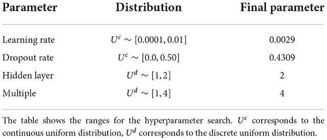
Table 6. Setup and final values of the hyperparameter search.

The constellation of column three (final parameter) in Table 6 is used to form the final network. For that, the network is trained on the training data, 20% of which is used for early stopping. Afterward the trained network is evaluated on the out-of-sample and on the out-of-time data. This procedure is repeated 25 times. Table 7 provides the average values and summarizes the evaluation of the different data sets and compares it across different models. Since the loss function in Eq. (8) depends on λ and p, changes in those parameters result in a loss of comparability.

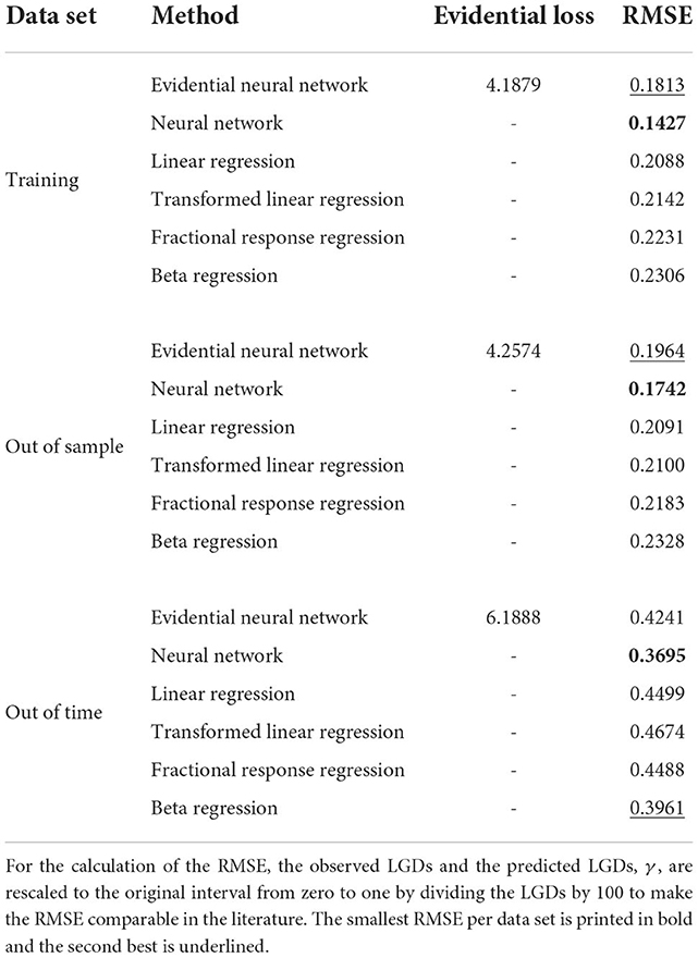
Table 7. Evaluation metrics.

Table 7 compares the neural network from the deep evidential framework to a neural network trained on the mean squared error and to common methods in the literature. These include the linear regression, the transformed linear regression, the beta regression, and the fractional response regression, see, e.g., [5, 14]. For the transformed linear regression the LGDs are transformed by a logit transformation, which is then used to fit a linear regression. The predictions of this regression are transformed back to their original scale using the sigmoid function. Each model is trained on the same training data. For the neural network trained with mean squared error, the same grid search and cross-validation approach with early stopping is used⁶. Since the evidential neural network is the only model with the marginal likelihood as an objective function the evidential loss can only be computed for this model. To compare the evidential neural network with different models, we evaluated the models using the root mean squared error. Note that for computing the root mean squared error only one parameter, γ, is needed since this parameter represents the prediction in terms of the LGD. From Table 7, we can see that the neural networks perform best on the training and the out-of-sample data. For the out-of-time data, the beta regression scores second best after the neural network trained with mean squared error, but the difference to the evidential neural networks is on the third digit.

4.2. Aleatoric and epistemic uncertainty in predictions

The deep evidential regression framework allows us to directly calculate the aleatoric and epistemic uncertainty for every prediction of our neural network. Figure 2 shows both types for our estimation sample. The x-axis shows the observation number for the predictions sorted in ascending order. The ordered LGDs are on the y-axis. The dark gray band around the ordered prediction is calculated by adding/subtracting the values of Eqs. (9) and (10) on our predictions. The light gray band is obtained by adding/subtracting two times the value of these equations. In the following, we call this “applying one or two standard errors of uncertainty” onto our predictions. The gray dots show the actual observed, i.e., true LGD realizations.

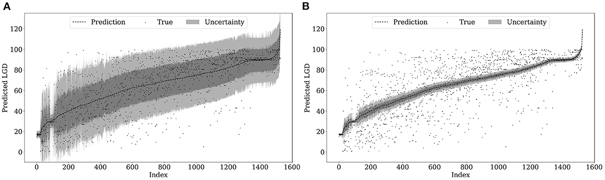
Figure 2. Uncertainty estimation in sample. (A) Aleatoric uncertainty. (B) Epistemic uncertainty.

Comparing the two plots of Figure 2, we observe that the aleatoric uncertainty covers a much larger range around our predictions than the epistemic uncertainty. Almost all true LGD realizations lie within the two standard errors of aleatoric uncertainty. Hence, the irreducible error or data uncertainty has the largest share of the total uncertainty. Recall that market-based LGDs are based on market expectations as they are calculated as 1 minus the traded market price 30 days after default. Therefore, the variation of the data also depends on market expectations which are notoriously difficult to estimate and to a large extent not predictable. Thus, it is reasonable that the aleatoric uncertainty is the main driver of the overall uncertainty. In contrast, the epistemic uncertainty, i.e., the model uncertainty, is considerably lower. This may be attributed to our database. This article covers nearly three decades including several recessions and upturns. Hence, we cover LGDs in many different points of the business cycle and across many industries and default reasons. Therefore, the data might be representative for the data generating process of market-based LGDs. Hence, the uncertainty due to limited sample size is relatively small in our application.

As we model all parameters of the evidential distribution dependent on the input features, we can also predict uncertainty for predictions in out-of-sample and out-of-time samples. Comparing Figures 2, 3 one might have expected that the epistemic uncertainty is increasing due to the lower sample size and the usage of unseen data. However, the functional relation of the epistemic uncertainty is calibrated on the estimation sample and transferred via prediction onto the out-of-sample data. Hence, if the feature values do not differ dramatically, the predicted uncertainty is similar. Only if we observe new realizations of our features in unexpected (untrained) value ranges, the uncertainty prediction should deviate strongly. Thus, we may use the prediction of the uncertainty also as a qualitative check of structural changes.

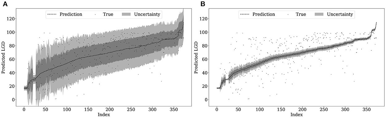
Figure 3. Uncertainty estimation out-of-sample. (A) Aleatoric uncertainty. (B) Epistemic uncertainty.

Structural changes in LGD estimation are primarily due to changes over time. This is one reason why some researchers argue to validate forecasting methods especially on out-of-time data sets, see, e.g., [3, 8]. In our application, there is no qualitative sign of structural breaks via diverging uncertainty estimates in 2018 and 2019. Comparing Figure 4 with the former two, we observe a similar pattern. This might have been expected as the out-of-time-period is not known for specific crises or special circumstances.

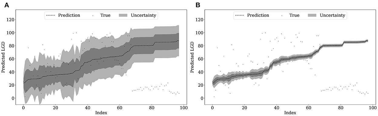
Figure 4. Uncertainty estimation out-of-time. (A) Aleatoric uncertainty. (B) Epistemic uncertainty.

Comparing the course of the epistemic uncertainty in all three figures, we observe that the uncertainty bands become smaller as the predicted LGD values increase. This implies that the neural network becomes more confident in predicting larger LGDs. Comparing this course with the histogram in Figure 1, one explanation for that might be the considerably larger sample size on the right-hand side. As we observe larger LGDs in our sample, the epistemic uncertainty in this area decreases.

4.3. Explaining LGD predictions

In this subsection, we take a deep dive into the drivers of the mean LGD predictions. As outlined in Section 3, we use ALE Plots to visualize the impact of our continuous features. We choose K = 10 buckets for all ALE plots. Overall we have three different sets of drivers. The first one consists of bond specific variables, subsequently we investigate drivers that reflect the overall macroeconomic developments and finally we follow Gambetti et al. [4] and include uncertainty-related variables. Evaluating the feature effects is important to validate that the inner mechanics of the uncertainty-aware neural network coincide with the economic intuitions. This is of major concern if financial institutions are tempted to use this framework for their capital requirement calculation. The requirement of explaining employed models is documented in many publications of regulatory authorities, see, e.g., [66–69].

Figure 5 shows the feature effect of bond-related drivers. The feature value range including a rugplot to visualize the distribution of the feature is shown on the x-axis. The effect of the driver on the LGD prediction is shown on the y-axis. We observe on the left-hand side of Figure 5, a negative effect of the coupon rate up to a value of roughly 8%. This negative relation seems plausible as higher coupon rates may also imply higher reflows during the resolution of the bond and, thus decreases the Loss Given Default. The relation starts to become positive after 8%, which may be explained by the fact that a higher coupon rate also implies higher risk and, thus the potential reflow becomes more uncertain. Maturity has an almost linear and positive relation with the predicted LGD values. In general, the increase in LGD with longer maturity is explained by sell-side pressure from institutional investors which usually hold bonds with a longer maturity, see, e.g., [48]. These relations were also confirmed by Gambetti et al. [4], who find that bond-related variables have a significant impact on the mean market-based LGD.

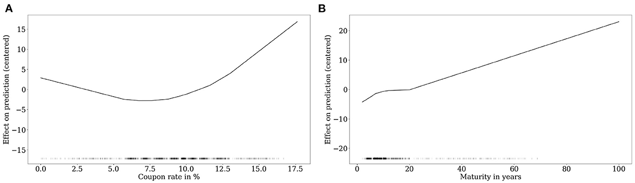
Figure 5. Bond-related drivers. (A) Coupon rate. (B) Maturity.

With regard to features that describe the macroeconomic surrounding, Figure 6 shows their effect on the LGD prediction. The default rate is one of the best-known drivers of market-based LGDs and is used in various studies, see, e.g., [3, 4, 30, 52]. The increasing course reflects the observation that LGDs tend to be higher in recession and crisis periods than in normal periods. This empirical fact also paves the way for generating so-called downturn estimates which should reflect this crisis behavior. These downturn estimates are also included in the calculation of the capital requirements for financial institutions, see, e.g., [70, 71] or for downturn estimates of EAD see Betz et al. [72]. Similarly, we observe a negative relation of predicted LGDs and S&P 500 returns, implying that LGDs increase if the returns become negative. Interestingly, positive returns have little impact on LGD predictions, which again, reinforces the downturn character of LGDs.

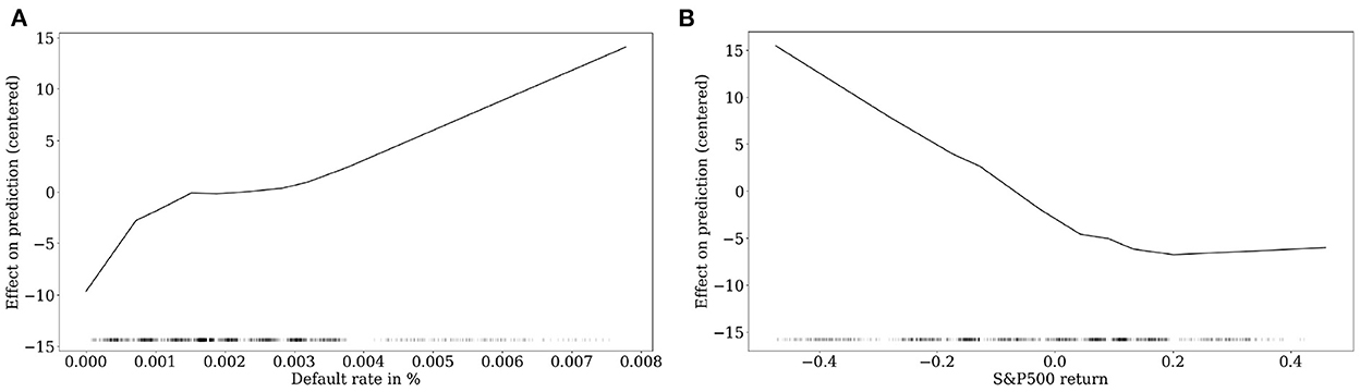
Figure 6. Macroeconomy-related drivers. (A) Default rate. (B) S&P 500 return.

Consistent with Gambetti et al. [4], who were the first to document the importance of uncertainty-related variables in the estimation of LGDs, we include two frequently used drivers as well, shown in Figure 7. Financial uncertainty proposed by Jurado et al. [44] and the News-based EPU index by Baker et al. [46], which cover uncertainty based on fundamental financial values and news articles. Both show a rather flat course from the low to mid of their feature value range. However, there is a clear positive impact on LGDs when the uncertainty indices reach high levels. Again, this reinforces the crisis behavior of market-based LGDs. The importance of uncertainty-related variables is also confirmed by Sopitpongstorn et al. [9] who find a significant impact as well. In a similar sense, Nazemi et al. [30] use news text-based measures for predicting market-based LGDs and underlining their importance. To summarize, recent literature suggests that uncertainty-related variables should be used to include all kinds of expectations of the economics surrounding the model framework.

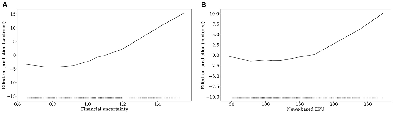
Figure 7. Uncertainty-related drivers. (A) Financial uncertainty. (B) News-based EPU.

5. Conclusion

Uncertainty estimation has become an active research domain in statistics and machine learning. However, there is a lack of quantification of uncertainty when applying machine learning to credit risk. This article investigates a recently published approach called Deep Evidential Regression by Amini et al. [42] and its extension by Meinert et al. [43]. This uncertainty framework has several advantages. First, it is easy to implement as one only has to change the loss function of the (deep) neural network and sightly adjust the output layer. Second, the predicted parameters of the adjusted network can easily be turned into mean prediction, aleatoric uncertainty, and epistemic uncertainty predictions. There are virtually no additional computational burdens to calculate predictions and their accompanying uncertainty. Third, the overall computational expense is much lower compared to approaches like Bayesian neural networks, ensemble methods, and bootstrapping. Furthermore, deep evidential regression belongs to a small class of frameworks which allow a direct, analytical disentangling of aleatoric and epistemic uncertainty. With these advantages, this framework may also be suitable for applications in financial institutions to accompany the usage of explainable artificial intelligence methods with quantification of aleatoric and epistemic uncertainty. Moreover, it is possible to include other variables, such as firm-specific financial risk factors, or to focus on non-listed companies. Further applications may also include the prediction of risk premiums in other asset pricing or forecasting the sale prices of real estate. Moreover, in other areas where predictions are critical such as health care, the quantification of prediction uncertainty may allow a broader application of machine learning methods.

This article uses almost 30 years of bond data to investigate the suitability of deep evidential regression on the challenging task of estimating market-based LGDs. The performance of the uncertainty-aware neural network is comparable to earlier literature and, thus, we do not see a large trade-off between accuracy and uncertainty quantification. This paper documents a novel finding regarding the ratio of aleatoric and epistemic uncertainty. Our results suggest that aleatoric uncertainty is the main driver of the overall uncertainty in LGD estimation. As this type is commonly known as the irreducible error, this gives rise to the conjecture that LGD estimation is notoriously difficult due to the high amount of data uncertainty. On the other hand, epistemic uncertainty that can be reduced or even set to zero with enough data plays only a minor role. Hence, the advantage of more complex and advanced methods, like machine learning, may be limited. However, this may not hold for all LGD data sets or if we look at different parts or parameters of the distribution other than the mean. Therefore, we do not argue that our results should be generalized to all aspects of LGDs, but are the first important steps to investigating the relation of aleatoric and epistemic uncertainty. Overall, understanding the determinants of both uncertainties can be key to getting a deeper understanding of the underlying process of market-based LGDs and, thus is certainly a fruitful path of future research.

Data availability statement

The data analyzed in this study is subject to the following licenses/restrictions: We do not have permission to provide the data. Requests to access these datasets should be directed to maximilian.nagl@ur.de.

Author contributions

MatN: conceptualization, methodology, software, formal analysis, and writing—original draft. MaxN: conceptualization, methodology, data curation, software, formal analysis, and writing—original draft. DR: conceptualization, methodology, resources, formal analysis, and writing—review and editing. All authors contributed to the article and approved the submitted version.

Funding

The publication was supported by the funding program Open Access Publishing (DFG).

Acknowledgments

We would like to thank the referees for their comments and suggestions that have substantially improved the article.

Conflict of interest

The authors declare that the research was conducted in the absence of any commercial or financial relationships that could be construed as a potential conflict of interest.

Publisher's note

All claims expressed in this article are solely those of the authors and do not necessarily represent those of their affiliated organizations, or those of the publisher, the editors and the reviewers. Any product that may be evaluated in this article, or claim that may be made by its manufacturer, is not guaranteed or endorsed by the publisher.

Footnotes

References

1. European Banking Authority. Risk Assessment of the European Banking System. (2021). Available online at: https://www.eba.europa.eu/risk-analysis-and-data/risk-assessment-reports
2. Altman EI, Kalotay EA. Ultimate recovery mixtures. J Bank Finance. (2014) 40:116–29. doi: 10.1016/j.jbankfin.2013.11.021
3. Kalotay EA, Altman EI. Intertemporal forecasts of defaulted bond recoveries and portfolio losses. Rev Finance. (2017) 21:433–63. doi: 10.1093/rof/rfw028
4. Gambetti P, Gauthier G, Vrins F. Recovery rates: uncertainty certainly matters. J Bank Finance. (2019) 106:371–83. doi: 10.1016/j.jbankfin.2019.07.010
5. Bellotti A, Brigo D, Gambetti P, Vrins F. Forecasting recovery rates on non-performing loans with machine learning. Int J Forecast. (2021) 37:428–44. doi: 10.1016/j.ijforecast.2020.06.009
6. Kellner R, Nagl M, Rösch D. Opening the black box–Quantile neural networks for loss given default prediction. J Bank Finance. (2022) 134:106334. doi: 10.1016/j.jbankfin.2021.106334
7. Bastos JA, Matos SM. Explainable models of credit losses. Eur J Oper Res. (2021) 301:386–94. doi: 10.1016/j.ejor.2021.11.009
8. Olson LM, Qi M, Zhang X, Zhao X. Machine learning loss given default for corporate debt. J Empir Finance. (2021) 64:144–59. doi: 10.1016/j.jempfin.2021.08.009
9. Sopitpongstorn N, Silvapulle P, Gao J, Fenech JP. Local logit regression for loan recovery rate. J Bank Finance. (2021) 126:106093. doi: 10.1016/j.jbankfin.2021.106093
10. Fraisse H, Laporte M. Return on investment on artificial intelligence: the case of bank capital requirement. J Bank Finance. (2022) 2022:106401. doi: 10.1016/j.jbankfin.2022.106401
11. Qi M, Yang X. Loss given default of high loan-to-value residential mortgages. J Bank Finance. (2009) 33:788–99. doi: 10.1016/j.jbankfin.2008.09.010
12. Bastos JA. Forecasting bank loans loss-given-default. J Bank Finance. (2010) 34:2510–17. doi: 10.1016/j.jbankfin.2010.04.011
13. Bellotti T, Crook J. Loss given default models incorporating macroeconomic variables for credit cards. Int J Forecast. (2012) 28:171–82. doi: 10.1016/j.ijforecast.2010.08.005
14. Loterman G, Brown I, Martens D, Mues C, Baesens B. Benchmarking regression algorithms for loss given default modeling. Int J Forecast. (2012) 28:161–70. doi: 10.1016/j.ijforecast.2011.01.006
15. Qi M, Zhao X. Comparison of modeling methods for loss given default. J Bank Finance. (2012) 35:2842–55. doi: 10.1016/j.jbankfin.2011.03.011
16. Tong ENC, Mues C, Thomas L. A zero-adjusted gamma model for mortgage loan loss given default. Int J Forecast. (2013) 29:548–62. doi: 10.1016/j.ijforecast.2013.03.003
17. Krüger S, Rösch D. Downturn LGD modeling using quantile regression. J Bank Finance. (2017) 79:42–56. doi: 10.1016/j.jbankfin.2017.03.001
18. Tomarchio SD, Punzo A. Modelling the loss given default distribution via a family of zero-and-one inflated mixture models. J R Stat Soc. (2019) 182:1247–66. doi: 10.1111/rssa.12466
19. Li Y, Chen W. Entropy method of constructing a combined model for improving loan default prediction: a case study in China. J Operat Res Soc. (2021) 72:1099–109. doi: 10.1080/01605682.2019.1702905
20. Petropoulos A, Siakoulis V, Stavroulakis E, Vlachogiannakis NE. Predicting bank insolvencies using machine learning techniques. Int J Forecast. (2020) 36:1092–113. doi: 10.1016/j.ijforecast.2019.11.005
21. Luo J, Yan X, Tian Y. Unsupervised quadratic surface support vector machine with application to credit risk assessment. Eur J Oper Res. (2020) 280:1008–17. doi: 10.1016/j.ejor.2019.08.010
22. Gunnarsson BR, vanden Broucke S, Baesens B, Óskarsdóttir M, Lemahieu W. Deep learning for credit scoring: do or don't? Eur J Oper Res. (2021) 295:292–305. doi: 10.1016/j.ejor.2021.03.006
23. Dumitrescu E, Hué S, Hurlin C, Tokpavi S. Machine learning for credit scoring: improving logistic regression with non-linear decision-tree effects. Eur J Oper Res. (2022) 297:1178–92. doi: 10.1016/j.ejor.2021.06.053
24. Kvamme H, Sellereite N, Aas K, Sjursen S. Predicting mortgage default using convolutional neural networks. Expert Syst Appl. (2018) 102:207–17. doi: 10.1016/j.eswa.2018.02.029
25. Barbaglia L, Manzan S, Tosetti E. Forecasting loan default in europe with machine learning*. J Financial Economet. (2021) 2021, nbab010. doi: 10.1093/jjfinec/nbab010
26. Sadhwani A, Giesecke K, Sirignano J. Deep learning for mortgage risk*. J Financial Economet. (2021) 19:313–68. doi: 10.1093/jjfinec/nbaa025
27. Chen S, Guo Z, Zhao X. Predicting mortgage early delinquency with machine learning methods. Eur J Oper Res. (2021) 290:358–72. doi: 10.1016/j.ejor.2020.07.058
28. Matuszyk A, Mues C, Thomas LC. Modelling LGD for unsecured personal loans: decision tree approach. J Operat Res Soc. (2010) 61:393–8. doi: 10.1057/jors.2009.67
29. Kaposty F, Kriebel J, Löderbusch M. Predicting loss given default in leasing: a closer look at models and variable selection. Int J Forecast. (2020) 36:248–66. doi: 10.1016/j.ijforecast.2019.05.009
30. Nazemi A, Baumann F, Fabozzi FJ. Intertemporal defaulted bond recoveries prediction via machine learning. Eur J Oper Res. (2021) doi: 10.1016/j.ejor.2021.06.047
31. Calabrese R, Zanin L. Modelling spatial dependence for loss given default in peer-to-peer lending. Expert Syst Appl. (2022) 192:116295. doi: 10.1016/j.eswa.2021.116295
32. Sigrist F, Hirnschall C. Grabit: Gradient tree-boosted Tobit models for default prediction. J Bank Finance. (2019) 102:177–92. doi: 10.1016/j.jbankfin.2019.03.004
33. Der Kiureghian A, Ditlevsen O. Aleatory or epistemic? Does it matter? Struct Safety. (2009) 31:105–12. doi: 10.1016/j.strusafe.2008.06.020
34. Gawlikowski J, Tassi CRN, Ali M, Lee J, Humt M, Feng J, et al. A survey of uncertainty in deep neural networks. ArXiv:2107.03342 [cs, stat] (2022) doi: 10.48550/arXiv.2107.03342
35. Blundell C, Cornebise J, Kavukcuoglu K, Wierstra D. Weight uncertainty in neural network. In: International conferEnce on Machine Learning. (Lille: PMLR). (2015). p. 1613–22.
36. Gal Y, Ghahramani Z. Dropout as a bayesian approximation: representing model uncertainty in deep learning. In: international Conference on Machine Learning. (New York, NY: PMLR). (2016). p. 1050–9.
37. Mobiny A, Yuan P, Moulik SK, Garg N, Wu CC, Van Nguyen H. Dropconnect is effective in modeling uncertainty of bayesian deep networks. Sci Rep. (2021) 11:1–14. doi: 10.1038/s41598-021-84854-x
38. Krueger D, Huang CW, Islam R, Turner R, Lacoste A, Courville A. Bayesian hypernetworks. arXiv preprint arXiv:171004759. (2017) doi: 10.48550/arXiv.1710.04759
39. Lakshminarayanan B, Pritzel A, Blundell C. Simple and scalable predictive uncertainty estimation using deep ensembles. In: Advances in Neural Information Processing Systems. Vol. 30. (Long Beach, CA: Curran Associates, Inc.). (2017).
40. Valdenegro-Toro M. Deep sub-ensembles for fast uncertainty estimation in image classification. arXiv preprint arXiv:191008168. (2019) doi: 10.48550/arXiv.1910.08168
41. Wen Y, Tran D, Ba J. Batchensemble: an alternative approach to efficient ensemble and lifelong learning. arXiv preprint arXiv:200206715. (2020) doi: 10.48550/arXiv.2002.06715
42. Amini A, Schwarting W, Soleimany A, Rus D. Deep evidential regression. In: Advances in Neural Information Processing Systems. vol. 33. Curran Associates, Inc. (2020). p. 14927–37.
43. Meinert N, Gawlikowski J, Lavin A. The unreasonable effectiveness of deep evidential regression. ArXiv:2205.10060 [cs, stat]. (2022) doi: 10.48550/arXiv.2205.10060
44. Jurado K, Ludvigson SC, Ng S. Measuring uncertainty. Am Econ Rev. (2015) 105:1177–216. doi: 10.1257/aer.20131193
45. Ludvigson SC, Ma S, Ng S. Uncertainty and business cycles: exogenous impulse or endogenous response? Am Econ J Macroecon. (2021) 13:369–410. doi: 10.1257/mac.20190171
46. Baker SR, Bloom N, Davis SJ. Measuring economic policy uncertainty*. Q J Econ. (2016) 131:1593–636. doi: 10.1093/qje/qjw024
47. Meinert N, Lavin A. Multivariate deep evidential regression. ArXiv:2104.06135 [cs, stat] (2022). doi: 10.48550/arXiv.2104.06135
48. Jankowitsch R, Nagler F, Subrahmanyam MG. The determinants of recovery rates in the US corporate bond market. J Financ Econ. (2014) 114:155–77. doi: 10.1016/j.jfineco.2014.06.001
49. Tobback E, Martens D, Gestel TV, Baesens B. Forecasting Loss Given Default models: impact of account characteristics and the macroeconomic state. J Operat Res Soc. (2014) 65:376–92. doi: 10.1057/jors.2013.158
50. Nazemi A, Fatemi Pour F, Heidenreich K, Fabozzi FJ. Fuzzy decision fusion approach for loss-given-default modeling. Eur J Oper Res. (2017) 262:780–91. doi: 10.1016/j.ejor.2017.04.008
51. Miller P, Töws E. Loss given default adjusted workout processes for leases. J Bank Finance. (2018) 91:189–201. doi: 10.1016/j.jbankfin.2017.01.020
52. Nazemi A, Heidenreich K, Fabozzi FJ. Improving corporate bond recovery rate prediction using multi-factor support vector regressions. Eur J Oper Res. (2018) 271:664–75. doi: 10.1016/j.ejor.2018.05.024
53. Starosta W. Loss given default decomposition using mixture distributions of in-default events. Eur J Oper Res. (2021) 292:1187–99. doi: 10.1016/j.ejor.2020.11.034
54. Apley DW, Zhu J. Visualizing the effects of predictor variables in black box supervised learning models. J R Stat Soc B. (2020) 82:1059–86. doi: 10.1111/rssb.12377
55. Friedman JH. Greedy function approximation: a gradient boosting machine. Ann Stat. (2001) 29:1189–232. doi: 10.1214/aos/1013203451
56. Goldstein A, Kapelner A, Bleich J, Pitkin E. Peeking inside the black box: visualizing statistical learning with plots of individual conditional expectation. J Comput Graph Stat. (2015) 24:44–65. doi: 10.1080/10618600.2014.907095
57. Ribeiro MT, Singh S, Guestrin C. “Why Should I Trust You?”: explaining the predictions of any classifier. In: Proceedings of the 22nd ACM SIGKDD International Conference on Knowledge Discovery and Data Mining. KDD '16. New York, NY: Association for Computing Machinery (2016). p. 1135–44.
58. Lundberg S, Lee SI. A unified approach to interpreting model predictions. arXiv:170507874 [cs, stat]. (2017).
59. Alvarez-Melis D, Jaakkola TS. On the robustness of interpretability methods. arXiv preprint arXiv:180608049. (2018) doi: 10.48550/arXiv.1806.08049
60. Visani G, Bagli E, Chesani F, Poluzzi A, Capuzzo D. Statistical stability indices for LIME: obtaining reliable explanations for machine learning models. J Operat Res Soc. (2022) 73:91–101. doi: 10.1080/01605682.2020.1865846
61. Bussmann N, Giudici P, Marinelli D, Papenbrock J. Explainable AI in fintech risk management. Front Artif Intell. (2020) 3:26. doi: 10.3389/frai.2020.00026
62. Giudici P, Raffinetti E. Explainable AI methods in cyber risk management. Quality and Reliabil Eng Int. (2022) 38:1318–26. doi: 10.1002/qre.2939
63. Babaei G, Giudici P, Raffinetti E. Explainable artificial intelligence for crypto asset allocation. Finance Res Lett. (2022) 47:102941. doi: 10.1016/j.frl.2022.102941
64. Bussmann N, Giudici P, Marinelli D, Papenbrock J. Explainable machine learning in credit risk management. Comput Econ. (2021) 57:203–16. doi: 10.1007/s10614-020-10042-0
65. Giudici P, Raffinetti E. Shapley-Lorenz eXplainable artificial intelligence. Expert Syst Appl. (2021) 167:114104. doi: 10.1016/j.eswa.2020.114104
66. Bank of Canada. Financial System Survey. Bank of Canada (2018). Available online at: https://www.bankofcanada.ca/2018/11/financial-system-survey-highlights/
67. Bank of England. Machine Learning in UK Financial Services. Bank of England and Financial Conduct Authority (2019). Available online at: https://www.bankofengland.co.uk/report/2019/machine-learning-in-uk-financial-services
68. Basel Committee on Banking Supervision. High-level summary: BCBS SIG industry workshop on the governance and oversight of artificial intelligence and machine learning in financial services (2019). Available online at: https://www.bis.org/bcbs/events/191003_sig_tokyo.htm
69. Deutsche Bundesbank. The Use of Artificial Intelligence Machine Learning in the Financial Sector. (2020). Available online at: https://www.bundesbank.de/resource/blob/598256/d7d26167bceb18ee7c0c296902e42162/mL/2020-11-policy-dp-aiml-data.pdf
70. Calabrese R. Downturn Loss Given Default: Mixture distribution estimation. Eur J Oper Res. (2014) 237:271–77. doi: 10.1016/j.ejor.2014.01.043
71. Betz J, Kellner R, Rösch D. Systematic effects among loss given defaults and their implications on downturn estimation. Eur J Oper Res. (2018) 271:1113–44. doi: 10.1016/j.ejor.2018.05.059
Keywords: machine learning, explainable artificial intelligence (XAI), credit risk, uncertainty, loss given default
Citation: Nagl M, Nagl M and Rösch D (2022) Quantifying uncertainty of machine learning methods for loss given default. Front. Appl. Math. Stat. 8:1076083. doi: 10.3389/fams.2022.1076083
Received: 21 October 2022; Accepted: 18 November 2022;
Published: 15 December 2022.
Edited by:
Paolo Giudici, University of Pavia, ItalyReviewed by:
Paola Cerchiello, University of Pavia, ItalyArianna Agosto, University of Pavia, Italy
Copyright © 2022 Nagl, Nagl and Rösch. This is an open-access article distributed under the terms of the Creative Commons Attribution License (CC BY). The use, distribution or reproduction in other forums is permitted, provided the original author(s) and the copyright owner(s) are credited and that the original publication in this journal is cited, in accordance with accepted academic practice. No use, distribution or reproduction is permitted which does not comply with these terms.
*Correspondence: Maximilian Nagl, maximilian.nagl@ur.de