Optimization of Spectral Wavelets for Persistence-Based Graph Classification

1. Introduction

1.1. Background

Graph classification is a challenging problem in machine learning. Unlike data represented in Euclidean space, there is no easily computable notion of distance or similarity between graphs. As such, graph classification requires techniques that lie beyond mainstream machine learning techniques focused on Euclidean data. Much research has been conducted on methods such as graph neural networks (GNNs) [1] and graph kernels [2, 3] that embed graphs in Euclidean space in a consistent manner.

Recently, persistent homology [4, 5] has been applied as a feature map that explicitly represents topological and geometric features of a graph as a set of persistence diagrams (a.k.a. barcodes). In the context of our discussion, the persistent homology of a graph G = (V, E) depends on a vertex function f : V → ℝ. In the case where a vertex function is not given with the data, several schemes have been proposed in the literature to assign vertex functions to graphs in a consistent way. For example, vertex functions can be constructed using local geometric descriptions of vertex neighborhoods, such as discrete curvature [6], heat kernel signatures [7] and Weisfeiler–Lehman graph kernels [8].

However, it is often difficult to know a priori whether a heuristic vertex assignment scheme will perform well in addressing different data science problems. For a single graph, we can optimize the vertex function over |V| many degrees of freedom in ℝ^V. In recent years, there have been many other examples of persistence optimization in data science applications. The first two examples of persistence optimization are the computation of Fréchet mean of barcodes using gradients on Alexandrov spaces [9], and that of point cloud inference [10], where a point cloud is optimized so that its barcode fits a target fixed barcode. The latter is an instance of topological inverse problems (see Oudot and Solomon [11] for a recent overview of such). Another inverse problem is that of surface reconstruction [12]. Besides, in the context of shape matching [13], persistence optimization is used in order to learn an adequate function between shapes. Finally, there are also many recent applications of persistence optimization in Machine Learning, such as the incorporation of topological information in Generative Modeling [14–16] or in Image Segmentation [17, 18], the design of topological losses for Regularization in supervised learning [19] or for dimension reduction [20].

Each of these applications can be thought of as minimizing a certain loss function over a manifold ${M}$ of parameters:

where ${L}:{M}\to {\text{Bar}}^N\to ℝ$ factors through the space Bar^N of N-tuples of barcodes. The aim is to find the parameter θ that best fits the application at hand. Gradient descent is a very popular approach in minimization, but it requires the ability to differentiate the loss function. In fact, Leygonie et al. [21] provide notions of differentiability for maps in and out Bar that are compatible with smooth calculus, and show that the loss functions ${L}$ corresponding the applications cited in the above paragraph are generically differentiable. The use of (stochastic) gradient descent is further legitimated by Carriere et al. [22], where convergence guarantees on persistence optimization problems are devised, using a recent study of stratified non-smooth optimization problems [23]. In practice, the minimization of ${L}$ can be unstable due to its non-convexity and partial non-differentiability. Some research has been conducted in order to smooth and regularize the optimization procedure [24, 25].

In a supervised learning setting, we want to optimize our vertex function assignment scheme over many individual graphs in a dataset. Since graphs may not share the same vertex set and come in different sizes, optimizing over the |V| degrees of freedom of any one graph is not conducive to learning a vertex function assignment scheme that can generalize to another graph. The degrees of freedom in any practical vertex assignment scheme should be independent of the number of vertices of a graph. However, a framework for parameterizing and optimizing the vertex functions of many graphs over a common parameter space ${M}$ is not immediately apparent.

The first instance of a graph persistence optimization framework (GFL) [26] uses a one layer graph isomorphism network (GIN) [1] to parameterize vertex functions. The GIN learns a vertex function by exploiting the local topology around each vertex. In this paper, we propose a different framework for assigning and parameterizing vertex functions, based on a graph's Laplacian operator. Using the Laplacian, we can explicitly take both local and global structures of the graph into consideration in an interpretable and transparent manner.

1.2. Outline and Contributions

We address the issue of vertex function parameterization and optimization using wavelet signatures. Wavelet signatures are vertex functions derived from the eigenvalues and eigenvectors of the graph Laplacian and encode multiscale geometric information about the graph [27]. The wavelet signature of a graph is dependent on a choice of wavelet g : ℝ → ℝ, a function on the eigenvalues of the graph's Laplacian matrix. We can thus obtain a parameterization of vertex functions for any graph $\mathrm{\text{F}}:{M}\to {ℝ}^V$ by parameterizing g. Consequently, the extended persistence of a graph—which has only four non-trivial persistence diagrams—can be varied over the parameter space ${M}$. If we have a function $\text{Out}$ : Bar⁴ → ℝ on persistence diagrams that we wish to minimize, we can optimize over ${M}$ to minimize the loss function

If ${L}$ is generically differentiable, we can optimize the wavelet signature parameters $\theta \in {M}$ using gradient descent methods. We illustrate an application of this framework to a graph classification problem in Figure 1, where the loss function ${L}$ is the classification error of a graph classification prediction model based on the graph's extended persistence diagrams.

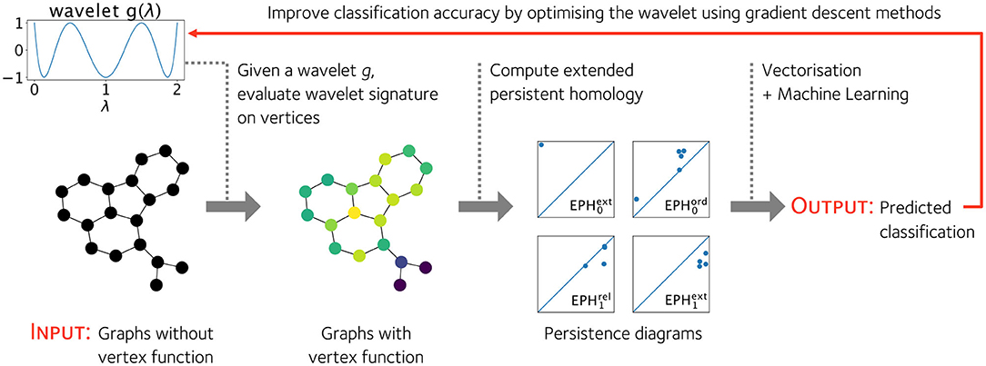
Figure 1. Given a wavelet g : ℝ → ℝ, we can equip any graph with a non-trivial vertex function. This allows us to compute the extended persistence diagrams of a graph and use the diagrams as features of the graph to predict a graph's classification in some real world setting. The wavelet g can be optimized to improve the classification accuracy of a graph classification pipeline based on the extended persistence diagrams of a graph's vertex function.

In section 2, we describe the assignment of vertex functions $\mathrm{\text{F}}:{M}\to {ℝ}^V$ by reviewing the definition of wavelet signatures. While spectral wavelets have been used in graph neural network architectures that predict vertex features [1] and compress vertex functions [28], they have not been considered in a persistent homology framework for graph classification. We describe several ways to parameterize wavelets. We also show in Proposition 2.2 that wavelet signatures are independent of the choice of eigenbasis of the graph Laplacian from which it is derived, ensuring that it is well-defined. We prove this result in Appendix B in Supplementary Material.

In section 3, we describe the theoretical basis for optimizing the extended persistent homology of a vertex function $\text{EPH}$ : ℝ^V → Bar⁴ and elucidate what it means for ${L}$ to be differentiable. In Proposition 3.3, we generalize the differentiability formalism of ordinary persistence [21] to extended persistence. We prove this result in Appendix A in Supplementary Material.

Finally, in section 4, we apply our framework to graph classification problems on several benchmark datasets. We show that our model is competitive with state-of-the-art persistence-based models. In particular, optimizing the vertex function appreciably improves the prediction accuracy on some datasets.

2. Filter Function Parameterization

We describe our recipe for assigning vertex functions to any simplicial graph G = (V, E) based on a parameterized spectral wavelet, the first part F of the loss function

Our recipe is based on a graph's wavelet signature, a vertex function derived from the graph's Laplacian. The wavelet signature also depends on a so-called ‘wavelet function’ in g : ℝ → ℝ, which is independent of the graph. By modulating the wavelet, we can jointly vary the wavelet signature across many graphs. We parameterize the wavelet using a finite linear combination of basis functions, such that the wavelet signature can be manipulated in a computationally tractable way. In the following section, we define the wavelet signature and describe our linear approach to wavelet parameterization.

2.1. Wavelet Signatures

The wavelet signature is a vertex function initially derived from wavelet transforms of vertex functions on graphs [29], a generalization of wavelet transforms for square integrable functions on Euclidean space [30, 31] for signal analysis [32]. Wavelet signatures for graphs have been applied to encode geometric information about meshes of 3D shapes [27, 32]. Special cases of wavelets signatures, such as the heat kernel signature [33] and wave kernel signature [34], have also been applied to describe graphs and 3D shapes [35, 36].

The wavelet signature of a graph is constructed from the graph's Laplacian operator. A graph's normalized Laplacian L ∈ ℝ^{V × V} is a symmetric positive semi-definite matrix, whose entries are given by

where k_u is the degree of vertex u. The Laplacian's eigenvalues λ and eigenvectors ϕ are known to encode various topological and geometric information about the graph [37, 38]; for example, the number of zero eigenvalues corresponds to the number of connected components of the graph. The spectrum of the normalized Laplacian have real eigenvalues in [0, 2] [37]. As such, any function g : ℝ → ℝ evaluated on the eigenvalues need only be defined on [0, 2]. Moreover, functions on a compact domain are easily parameterized using convenient bases.

Definition 2.1. (Wavelet Signature [27]) Let L ∈ ℝ^{V × V} be the normalized Laplacian of a simplical graph G = (V, E). Let ϕ₁, …, ϕ_|V| be an orthonormal eigenbasis for L and λ₁, …, λ_|V| be their corresponding eigenvalues. The wavelet signature W : ℝ^{[0, 2]} → ℝ^V maps a function g : [0, 2] → ℝ, which we refer to as a wavelet, to a vertex function W(g) ∈ ℝ^V linearly, where the value of W(g) on vertex v is given by

and (ϕ_i)_v denotes the component of eigenvector ϕ_i corresponding to vertex v.

If the eigenvalues of L have geometric multiplicity one (i.e., their eigenspaces are one dimensional), then the orthonormal eigenvectors are uniquely defined up to a choice of sign. It is then apparent from Equation (3) that the wavelet signature is independent of the choice of sign. However, if some eigenvalues have geometric multiplicity greater than one, then the orthonormal eigenvectors of L are uniquely defined up to orthonormal transformations in the individual eigenspaces. However, the wavelet signature is well-defined even when the multiplicities of eigenvalues are greater than one. This is the content of the next Proposition, whose proof is deferred to Appendix B in Supplementary Material.

PROPOSITION 2.2. The wavelet signature of a graph is independent of the choice of orthonormal eigenbasis for the Laplacian.

Remark 2.3. In addition to the traditional view of wavelets from a spectral signal processing perspective [29], we can also relate the wavelet signature of a vertex v to the degrees of vertices in some neighborhood of v prescribed by g. Consider a wavelet g : [0, 2] → ℝ. On a finite graph G, the normalized Laplacian L has at most |V| many distinct eigenvalues. As such, there exists a polynomial $ĝ(x)=\sum _{n=0}^p{a}_n{x}^n$ of finite order that interpolates g at the eigenvalues g(λ_i) = ĝ(λ_i). Therefore, W(g) = W(ĝ). Moreover, the vertex values assigned by W(ĝ) are the diagonal entries of the matrix polynomial ĝ(L):

Furthermore, we can also write the matrix polynomial ĝ(L) as a matrix polynomial in A = I − L, the normalized adjacency matrix. From the definition of L, we can compute the diagonal entry of a monomial A^r corresponding to vertex v as an inverse degree weighted count of paths¹ [v₀, v₁, …, v_r] on the graph which begin and end on vertex v = v₀ = v_r [39]:

By expressing the wavelet signature as a matrix polynomial in A, we see that g controls how information at different length scales of the graph contribute to the wavelet signature. For instance, if g were an order p polynomial, then W(g)_v only takes the degrees of vertices that are ⌊p/2⌋ away from v into account. As a corollary, since W(g) can be specified by replacing g with a polynomial ĝ of order at most |V| − 1, the wavelet signature at a vertex is only dependent on the subgraph of G that is within ⌊|V| − 1⌋/2 steps away from v.

2.2. Parameterizing the Wavelet

We see from Remark 2.3 that the choice of wavelet g determines how the topology and geometry of the graph is reflected in the vertex function. Though the space of wavelets is potentially infinite dimensional, here we only consider wavelets g_θ(x) that are parameterized by parameters θ in a finite dimensional manifold, so that we can easily optimize them using computational methods. In particular, we focus on wavelets written as a linear combination of m basis functions h₁, …, h_m : [0, 2] → ℝ

This parameterization of wavelets in turn defines a parameterization of vertex functions F : ℝ^m → ℝ^V for our optimization pipeline in Equation (1)

Since W(g) is a linear function of the wavelet g, F is a linear transformation:

We can write F as a |V| × m matrix acting on a vector ${\left[{\theta }_1,\dots {\theta }_m\right]}^{⊺}\in {ℝ}^m$, whose columns are the vertex functions W(h_j).

Example 2.4 (Chebyshev Polynomials). Any Lipschitz continuous function on an interval can be well-approximated by truncating its Chebyshev series at some finite order [40]. The Chebyshev polynomials T_n : [−1, 1] → ℝ

form an orthonormal set of functions. We can thus consider h_j(λ) = T_j(λ − 1), j = 0, 2, …, m as a naïve basis for wavelets. We exclude T₁(x) = x in the linear combination as W(T₁(1 − x)) = 0 for graphs without self loops.

Example 2.5 (Radial Basis Functions). In the machine learning community, a radial function refers loosely to a continuous monotonically decreasing function ρ : ℝ_≥0 → ℝ_≥0. There are many possible choices for ρ, for example, the inverse multiquadric

where ϵ ≠ 0 is a width parameter. We can obtain a naïve wavelet basis h_j(x) = ρ(||x − x_j||) using copies of ρ offset by a collection of centroids x_j ∈ ℝ along ℝ. In general, the centroids are parameters that could be optimized, but we fix them in this study. This parameterization can be considered as a radial basis function neural network. RBNNs are well-studied in function approximation and subsequently machine learning; we refer readers to [41, 42] for further details.

2.3. The Choice of Wavelet Basis

The choice of basis functions determines the space of wavelet signatures and also the numerical stability of the basis function coefficients which serve as the wavelet signature parameters. The stability of the parameterization depends on the graphs as much as the choice of wavelet basis h₁, …, h_m. We can analyse the stability of a parameterization F by its the singular value decomposition

where σ₁, …, σ_r are the non-zero singular values of the matrix, and $u_k\in {ℝ}^{\left|V\right|}$ and $v_k\in {ℝ}^m$ are orthonormal sets of vectors, respectively. If the distribution of singular values span many orders of magnitude, we say the parameterization is ill-conditioned. An ill-conditioned parameterization interferes with the convergence of gradient descent algorithms on a loss function evaluated on wavelet signatures. We discuss the relationship between the conditioning of F and the stability of gradient descent in detail in Remark 2.7.

We empirically observe that the coefficients of a naïve choice of basis functions, such as Chebyshev polynomials or radial basis functions, are numerically ill-conditioned. In Figure A2 (Appendix in Supplementary Material.), we can see that the singular values of radial basis function and Chebyshev polynomial parameterizations, respectively, are distributed across a large range on the logarithmic scale for some datasets of graphs in machine learning. We address this problem by picking out a new wavelet basis

where σ_k are the singular values of F and v_k are the associated vectors in ℝ^m from the singular value decomposition of matrix F in Equation (11). Then the parameterization F′ : ℝ^r → ℝ^V

have singular values equal to one, since this is a linear combination of orthonormal vectors $u_k\in {ℝ}^V$:

As an example, we plot the new wavelet basis $h_k^{\prime }$ derived from a 12 parameter radial basis function parameterization for the MUTAG dataset in Figure A3 in Appendix B in Supplementary Material.

Remark 2.6 (Learning a Wavelet Basis for Wavelet Signatures on Multiple Graphs). In the case where the wavelet coefficients parameterize the wavelet signatures over graphs G₁, …, G_N, we can view the maps F₁, …, F_N that map wavelet basis coefficients to vertex functions of graphs G₁, …, G_N, respectively, as a parameterization for the disjoint union ⊔_iG_i:

We can then perform a singular value decomposition of the parameterization F on ⊔_iG_i and derive a new, well-conditioned basis.

Remark 2.7 (Why the Conditioning of F Matters). Let us optimize a loss function ${L}$ on the parameter space of wavelet coefficients θ using a gradient descent algorithm. In a gradient descent step of step size s, the wavelet coefficients are updated to $\theta \mapsto \theta -s{\nabla }_{\theta }{L}$. Using the singular value decomposition of F (Equation 11), we can write

The change in the vertex function is simply the matrix F applied to the change in wavelet parameters. Hence, the vertex function is updated to $f\mapsto f-s\mathrm{\text{F}}{\nabla }_{\theta }{L}$, where

If the loss function ${L}$ has large second derivatives– for example, due to non-linearities in the function on persistence diagrams $\text{Out}$ : Bar⁴ → ℝ—the projections $\langle {\nabla }_f{L},u_k\rangle$ in Equations (16) and (17) may change dramatically from one gradient descent update to another. If the smallest singular value is much smaller than the largest, then updates to the wavelet signature can be especially unstable throughout the optimization process. This source of instability can be removed if we choose a parameterization with uniform singular values σ_k = 1. In this case, the update to f is simply the projection of ${\nabla }_f{L}$ onto the space of wavelet signatures spanned by u₁, …, u_r, without any distortion introduced by non-uniform singular values:

3. Extended Persistent Homology

The homology of a given graph is a computable vector space whose dimension counts the number of connected components or cycles in the graph. Finer information can be retained by filtering the graph and analyzing the evolution of the homology throughout the filtration. This evolution is described by a set of extended persistence diagrams (a.k.a. extended barcodes), a multiset of points 〈b, d〉 that record the birth b and death of homological features in the filtration. In this section, we begin by summarizing these constructions. We refer the reader to Zomorodian and Carlsson [4], Edelsbrunner and Harer [5], and Cohen-Steiner et al. [43] for full treatments of the theory of Persistence.

Compared to ordinary persistence, extended persistence is a more informative and convenient feature map for graphs. Extended persistence encodes strictly more information than ordinary persistence. For instance, the cycles of a graph are represented as points with d = ∞ in ordinary persistence. Thus, only the birth coordinate b of such points contain useful information about the cycles. In contrast, the corresponding points in extended persistence are each endowed with a finite death time d, thus associating extra information to the cycles. The points at infinity in ordinary persistence also introduce obstacles to vectorization procedures, as often arbitrary finite cutoffs are needed to ‘tame’ the persistence diagrams before vectorization.

3.1. Extended Persistent Homology

Let G = (V, E) be a finite graph without double edges and self-loops. For the purposes of this paper, the associated extended persistent homology is a map

from functions f ∈ ℝ^V on its vertices to the space of four persistence diagrams or barcodes, which we define below. The map arises from a filtration of the graph, a sequential attachment of vertices and edges in ascending or descending order of f. We extend f on each edge e = (v, v′) by the maximal value of f over the vertices v and v′, and we then let G_t ⊂ G be the sub graph induced by vertices taking value less than t. Then we have the following sequence of inclusions:

Similarly, the sub graphs G^t ⊂ G induced by vertices taking value greater than t assemble into a sequence of inclusions:

The changes in the topology of the graph along the filtration in ascending and descending order of f can be detected by its extended persistence module, indexed over the poset ℝ ∪ {∞} ∪ ℝ^op:

where H_p is the singular (relative) homology functor in degree p ∈ 0, 1 with coefficients in a fixed field, chosen to be ℤ/2ℤ in practice. In general terms, the modules $\text{V}$₀(f) and $\text{V}$₁(f) together capture the evolution of the connected components and loops in the sub graphs of G induced by the function f.

Each module $\text{V}$_p(f) is completely characterized by a finite multi-set $\text{EPH}$_p(f) of pairs of real numbers 〈b, d〉 called intervals representing the birth and death of homological features. Following Cohen-Steiner et al. [44], the intervals in $\text{EPH}$_p(f) are further partitioned according to the type of homological feature they represent:

Each of the three finite multiset ${\text{EPH}}_p^{\text{k}}(f)$, for k ∈ {ord, ext, rel}, is an element in the space Bar of so-called barcodes or persistence diagrams. However, ${\text{EPH}}_0^{\text{rel}}(f)$ and ${\text{EPH}}_1^{\text{ord}}(f)$ being trivial for graphs, we refer to the collection of four remaining persistence diagrams

as the extended barcode or extended persistence diagram of f. We have thus defined the extended persistence map

Remark 3.1. If we only apply homology to the filtration of Equation (19), we get an ordinary persistence module indexed over the real line, which is essentially the first row in Equation (21). This module is characterized by a unique barcode $\text{PH}$_p(f) ∈ Bar. We refer to the map

as the ordinary persistence map.

3.2. Differentiability of Extended Persistence

The extended persistence map can be shown to be locally Lipschitz by the Stability theorem [44]. The Rademacher theorem states that any real-valued function that is locally Lipschitz is differentiable on a full measure set. Thus, so is our loss function

as long as $\text{Out}$ and F are smooth or locally Lipschitz². If a loss function ${L}$ is locally Lipschitz, we can use stochastic gradient descent as a paradigm for optimization. Nonetheless, the theorem above does not rule out dense sets of non differentiability in general.

In this section, we show that the set where $\text{EPH}$ is not differentiable is not pathological. Namely, we show that $\text{EPH}$ is generically differentiable, i.e., differentiable on an open dense subset. This property guarantees that local gradients yield reliable descent directions in a neighborhood of the current iterate. We recall from Leygonie et al. [21] the definition of differentiability for maps to barcodes.

We call a map $\mathrm{\text{F}}:{M}\to {ℝ}^V$ a parameterization, as it corresponds to a selection of filter functions over G parameterized by the manifold ${M}$. Then B: = $\text{EPH}$ ◦ F is the barcode valued map whose differentiability properties are of interest in applications.

Definition 3.2. A map $B:{M}\to \text{Bar}$ on a smooth manifold ${M}$ is said to be differentiable at $\theta \in {M}$ if for some neighborhood U of θ, there exists a finite collection of differentiable maps³ b_i, d_i : U → ℝ ∪ {∞}, called a local coordinate system for B at θ, such that

For N ∈ ℕ, we say that a map $B:{M}\to {\text{Bar}}^N$ is differentiable at θ if all its components are so.

In Leygonie et al. [21], it is proven that the composition $\text{PH}$ ◦ F is generically differentiable as long as F is so. It is possible to show that $\text{EPH}$ ◦ F is generically differentiable along the same lines, but we rather provide an alternative argument in the Appendix. Namely, we rely on the fact that the extended persistence of G can be decoded from the ordinary persistence of the cone complex $\text{C}$(G), a connection first noted in Cohen-Steiner et al. [44] for computational purposes.

PROPOSITION 3.3. Let $\mathrm{\text{F}}:{M}\to {ℝ}^V$ be a generically differentiable parameterization. Then the composition $\text{EPH}$ ◦ F is generically differentiable.

For completeness, the proof provided in the Appendix treats the general case of a finite simplicial complex K of arbitrary dimension.

4. Binary Graph Classification

We investigate whether optimizing the extended persistence of wavelet signatures can be usefully applied to graph classification problems, where persistence diagrams are used as features to predict discrete, real life attributes of networks. In this setting, we aim to learn $\theta \in {M}$ that minimize the classification error of graphs over a training dataset.

We apply our wavelet optimization framework to classification problems on the graph datasets MUTAG [47, 48], COX2 [49], DHFR [49], NCI1 [50, 51], PROTEINS [52, 53], and IMDB-B [54]. The former five datasets are biochemical molecules and IMDB-B is a collection of social ego networks. In our models, we use persistence images [46] as a fixed vectorization method and use a feed forward neural network to map the persistence images to classification labels. We also include the eigenvalues of the graph Laplacian as additional features; model particulars are described in the sections below.

To illustrate the effect of wavelet optimization on different classification problems, we also perform a set of control experiments where for the same model architecture, we fix the wavelet and only optimize the parameters of the neural network. The control experiment functions as a baseline against which we assess the efficacy of wavelet optimization.

We benchmark our results with two existing persistence based architectures, PersLay [7] and GFL [26]. Perslay optimizes the vectorization parameters and use two heat kernel signatures as fixed rather than optimizable vertex functions for computing extended persistence. GFL optimizes and parameterizes vertex functions using a graph isomorphism network [1], and computes ordinary sublevel and superlevel set persistence instead of extended persistence.

4.1. Model Architecture

We give a high level description of our model and relegate details and hyperparameter choices of the vectorization method and neural network architecture to Appendix C in Supplementary Material. In our setting, the extended persistence diagrams of the optimizable wavelet signatures for each graph are vectorized as persistence images. We also include the static persistence images of a fixed heat kernel signature, W(e^−0.1x), as an additional set of features, alongside some non-persistence features. Both the optimized and static persistence diagrams are transformed into the persistence images using identical hyperparameters. We feed the optimizable and static persistence images into two separate convolutional neural networks (CNNs) with the same architecture. Similarly, we feed the non-persistence features as a vector into a separate multilayer perceptron. The outputs of the CNNs are concatenated with the outputs of the multi-layer perceptron. Finally, an affine transformation sends the concatenated vector to a real number whose sign determines the binary classification.

4.1.1. Wavelet Parametserization

We choose a space of wavelets spanned by 12 inverse multiquadric radial basis functions

whose centroids x_j are located at x_j = 2(j − 1)/9, j = 0, …, 11. The width parameter is chosen to be the distance between the centroids, ϵ = 2/9. On each dataset, we derive a numerically stable parameterization using the procedure described in section 2.2; the parameters we optimize are the coefficients of the new basis given by Equation (12). We initialize the parameters by fitting them via least squares to the heat kernel signature W(e^−10x) on the whole dataset of graphs.

4.1.2. Non-Persistence Features

We also incorporate the eigenvalues of the normalized Laplacian as additional, fixed features of the graph. Since the number of eigenvalues for a given graph is equal to the number of vertices, it differs between graphs in the same dataset. To encode the information represented in the eigenvalues as a fixed length vector, we first sort the eigenvalues into a time-series; we then compute the log path signature of the time series up to level four, which is a fixed length vector in ℝ⁸. The log-signature captures the geometric features of the path; we refer readers to Chevyrev and Kormilitzin [55] for details about path signatures. For IMDB-B in particular, we also include the maxima and minima of the heat kernel signatures W(e^−10x) and W(e^−0.1x), respectively, of each graph.

4.2. Experimental Set Up

We employ a 10 ten-fold test-train split scheme on each dataset to measure the accuracy of our model. Each ten-fold is a set of ten experiments, corresponding to a random partition of the dataset into ten portions. In each experiment, a different portion is selected as the test set while the model is trained on the remaining nine portions. We perform 10 ten-folds to obtain a total of 10 × 10 experiments, and report the accuracy of the classifier as the average accuracy over 100 such experiments. The epochs at which the accuracies were measured are specified in Table C1.

Across all experiments, we use binary cross entropy as the loss function. We use the Adam optimizer [56] with learning rate lr = 1e-3 to optimize the parameters of the neural network. The wavelet parameters are updated using stochastic gradient descent with learning rate lr = 1e-2, for all datasets except for IMDB-B, where the learning rate is set to lr = 1e-1. The batch sizes for each experiment are shown in Table C2. In all experiments, we stop the optimization of wavelet parameters at epoch 50 while the neural network parameters continue to be optimized.

We use the GUDHI library to compute persistence, and make use of the optimization and machine learning library PyTorch for the construction of the graph classifications models.

4.3. Results and Discussion

In Table 1, we present the classification accuracies of our model. For each dataset, we perform four experiments using our model, varying whether the wavelet parameter is optimized and whether additional features are included. In Table 2, we show the test accuracy of our model alongside two persistence-based graph classification architectures, Perslay and GFL, as well as other state-of-the-art graph classification architectures.

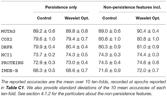
Table 1. Binary classification accuracy of our model where we vary whether non-Persistence features are included and whether the wavelet is optimized.

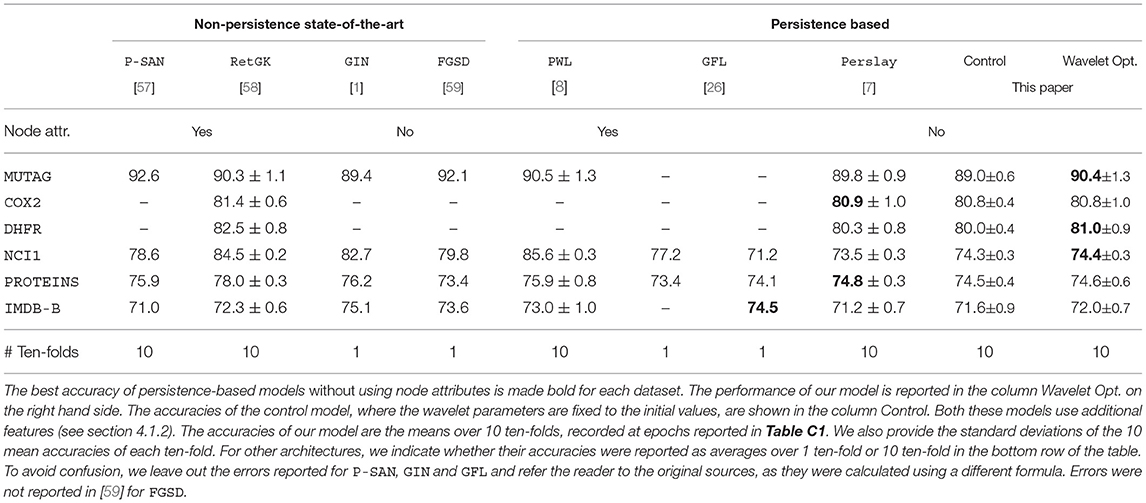
Table 2. Binary classification accuracy on datasets of graphs.

We first compare the performances of our model between cases where we optimize and fix the wavelets. In Table 1, we see that on MUTAG and DHFR, optimizing the wavelet improves the classification accuracy regardless of whether extra features are included. On NCI1, wavelet optimization improves the classification accuracy only persistence features are included. When we include non-persistence features in the model, the performances of the optimized and control models are statistically indistinguishable for NCI1, suggesting that the non-persistence features play a more significant role in the classification. As for COX2, PROTEINS, and IMDB-B, optimizing the wavelet coefficients do not bring about statistically significant improvements. This indicates that the initial wavelet signature—the heat kernel signature W(e^−10x)—is a locally optimal choice of wavelet for our neural network classifier.

We now compare our architecture to other persistence based architectures, Perslay and GFL, where node attributes are excluded from their vertex function models. Except on PROTEINS, our wavelet optimized model matches or exceeds Perslay. While our model architecture and choice of wavelet initialization is similar to that of Perslay, we differ in two important respects. Perslay fixes the vertex functions but optimizes the weights assigned to points on the persistence diagrams, as well as the parameters of the persistence images. Our improvements on Perslay for MUTAG, DHFR, and IMDB-B indicate that vertex function optimization yields improvements that cannot be obtained through vectorization optimization alone on some datasets of graphs.

Compared to GFL (without node attributes), both Perslay and our architecture achieves similar or higher classification accuracies on PROTEINS and NCI1. This supports wavelet signatures being viable models for vertex functions on those datasets. On the other hand, both Perslay and our model lag behind GFL on IMDB-B. We attribute this to the fact that IMDB-B, unlike the other bioinformatics datasets, consists of densely connected graphs. The graphs in IMDB-B have diameter at most two and 14% of the graphs are cliques. This fact has two consequences. First, we expect the one-layer GIN used in GFL—a local topology summary—to be highly effective in optimizing for the salient features of a graph with small diameter. Second, the extended persistence modules for cliques have zero persistence, since all vertices are assigned the same function value due to symmetry. In contrast, ordinary persistence used in GFL is able to capture the cycles in a complete graph as points with infinite persistence.

Compared to non-persistence state-of-the-art architectures in Table 1, our model achieves competitive accuracies on MUTAG, COX2, and DHFR. For NCI1 and PROTEINS, all persistence architectures listed that exclude additional node attributes perform poorly in comparison, though PWL was able to achieve leading results with node attributes.

All in all, we observe that wavelet signatures can be an effective parameterization of vertex functions when we use extended persistence as features for graph classification. In particular, on some bioinformatics datasets, we show that optimizing the wavelet signature can lead to improvements in classification accuracy. The wavelet signature approach is complementary to the GFL approach to vertex function parameterization as they show strengths on different datasets.

5. Conclusion

We have presented a framework for equipping any graph G with a set of extended persistence diagrams $\text{EPH}◦\mathrm{\text{F}}:{M}\to {\text{Bar}}^4$ parameterized over a manifold ${M}$, a parameter space for the graph's wavelet signature. We described how wavelet signatures can be parameterized and interpreted. Given a function on extended persistence diagrams $\text{Out}$ : Bar⁴ → ℝ that is differentiable, we have shown how a loss function ${L}=\text{Out}◦\text{EPH}◦\mathrm{\text{F}}$ can be generically differentiable with respect to $\theta \in {M}$ as ${L}$. Thus, we can apply gradient descent methods to optimize the extended persistence diagrams of a graph to minimize ${L}$.

We applied this framework to a graph classification architecture where the wavelet signature is optimized for classification accuracy. We are able to demonstrate an increase in accuracy on several benchmark datasets where the wavelet is optimized, and perform competitively with state-of-the-art persistence based graph classification architectures.

Data Availability Statement

The code for the computational experiments in section 4 can be found in the GitHub repository https://github.com/kmyim/Persistence_Opt_Spectral_Wavelets. The datasets we use are publicly available at the repository TUDatasets https://chrsmrrs.github.io/datasets/ [60].

Author Contributions

The overall framework was jointly conceived by both authors. KY was responsible for developing wavelet signatures as a vertex function parameterization framework, along with the experimental design and analysis. The proof of the differentiability of extended persistence is due to JL. Both authors participated in the writing of the article.

Funding

KY was funded by the EPSRC Centre For Doctoral Training in Industrially Focused Mathematical Modelling (EP/L015803/1) with industrial sponsorship from Elsevier. JL was funded by the EPSRC grant EP/R513295/1. Both authors are members of the Centre for Topological Data Analysis, which is supported by the EPSRC grant New Approaches to Data Science: Application Driven Topological Data Analysis EP/R018472/1.

Conflict of Interest

The authors declare that the research was conducted in the absence of any commercial or financial relationships that could be construed as a potential conflict of interest.

Acknowledgments

The authors would like to thank Ulrike Tillmann and Heather Harrington for their close guidance and thoughtful advice on this project. In addition, the authors would like to thank Vidit Nanda, Peter Grindrod CBE, Andrew Mellor, Steve Oudot, Mathieu Carrière, and Theo Lacombe for fruitful discussions on this subject. Finally, we are indebted to the reviewers for their thoughtful and constructive comments, which led to many improvements of the paper.

Supplementary Material

The Supplementary Material for this article can be found online at: https://www.frontiersin.org/articles/10.3389/fams.2021.651467/full#supplementary-material

Footnotes

References

1. Xu B, Shen H, Cao Q, Qiu Y, Cheng X. Graph wavelet neural network. arXiv [Preprint]. (2019) arXiv:1904.07785.
2. Vishwanathan SVN, Schraudolph NN, Kondor R, Borgwardt KM. Graph kernels. J Mach Learn. Res. (2010) 11:1201–42.
3. Shervashidze N, Vishwanathan SVN, Petri T, Mehlhorn K, Borgwardt K. Efficient graphlet kernels for large graph comparison. In: van Dyk D, Welling M, editors. Proceedings of the Twelfth International Conference on Artificial Intelligence and Statistics, Vol. 5. Clearwater Beach, FL: PMLR (2009). p. 488–95. Available online at: http://proceedings.mlr.press/v5/shervashidze09a.html
4. Zomorodian A, Carlsson G. Computing persistent homology. Discr Comput Geom. (2005) 33:249–74. doi: 10.1007/s00454-004-1146-y
5. Edelsbrunner H, Harer J. Persistent homology-a survey. Contemp Mathe. (2008) 453:257–82. doi: 10.1090/conm/453/08802
6. Zhao Q, Wang Y. Learning metrics for persistence-based summaries and applications for graph classification. In: Wallach H. Larochelle H, Beygelzimer A, d'Alché-Buc F, Fox E, Garnett R, editors. Advances in Neural Information Processing Systems, Vol. 32. Red Hook, NY: Curran Associates, Inc. (2019). p. 9859–70. Available online at: https://proceedings.neurips.cc/paper/2019/file/12780ea688a71dabc284b064add459a4-Paper.pdf
7. Carrière M, Chazal F, Ike Y, Lacombe T, Royer M, Umeda Y. Perslay: a neural network layer for persistence diagrams and new graph topological signatures. In: Chiappa S, Calandra R, editors. Proceedings of the Twenty Third International Conference on Artificial Intelligence and Statistics, Vol. 108. PMLR (2020). p. 2786–96. Available online at: http://proceedings.mlr.press/v108/carriere20a.html.
8. Rieck B, Bock C, Borgwardt K. A persistent weisfeiler-lehman procedure for graph classification. In: International Conference on Machine Learning. PMLR (2019). p. 5448–58.
9. Turner K, Mileyko Y, Mukherjee S, Harer J. Fréchet means for distributions of persistence diagrams. Discr Comput Geom. (2014) 52:44–70. doi: 10.1007/s00454-014-9604-7
10. Gameiro M, Hiraoka Y, Obayashi I. Continuation of point clouds via persistence diagrams. Phys D. (2016) 334:118–32. doi: 10.1016/j.physd.2015.11.011
11. Oudot S, Solomon E. Inverse problems in topological persistence. In: Baas NA. Carlsson GE, Quick G, Szymik M, Thaule M, editors. Topological Data Analysis. Cham: Springer (2020). p. 405–33. doi: 10.1007/978-3-030-43408-3_16
12. Brüel-Gabrielsson R, Ganapathi-Subramanian V, Skraba P, Guibas LJ. Topology-aware surface reconstruction for point clouds. Comp Graph Forum. (2020) 39:197–207. doi: 10.1111/cgf.14079
13. Poulenard A, Skraba P, Ovsjanikov M. Topological function optimization for continuous shape matching. Comp Graph Forum. (2018) 37:13–25. doi: 10.1111/cgf.13487
14. Moor M, Horn M, Rieck B, Borgwardt K. Topological autoencoders. In: International Conference on Machine Learning. PMLR (2020). p. 7045–54.
15. Hofer C, Kwitt R, Niethammer M, Dixit M. Connectivity-optimized representation larning via persistent homology. In: Chaudhuri K, Salakhutdinov R, editors. Proceedings of the 36th International Conference on Machine Learning. Long Beach, CA: PMLR (2019). p. 2751–60. Available online at: http://proceedings.mlr.press/v97/hofer19a.html
16. Gabrielsson RB, Nelson BJ, Dwaraknath A, Skraba P. A topology layer for machine learning. In: International Conference on Artificial Intelligence and Statistics. PMLR (2020). p. 1553–63.
17. Hu X, Li F, Samaras D, Chen C. Topology-preserving deep image segmentation. In: Advances in Neural Information Processing Systems. Red Hook, NY: Curran Associates, Inc. (2019). p. 5658–69. Available online at: https://proceedings.neurips.cc/paper/2019/file/12780ea688a71dabc284b064add459a4-Paper.pdf
18. Clough JR, Oksuz I, Byrne N, Schnabel JA, King AP. Explicit topological priors for deep-learning based image segmentation using persistent homology. In: International Conference on Information Processing in Medical Imaging. Hong Kong: Springe (2019). p. 16–28. doi: 10.1007/978-3-030-20351-1_2
19. Chen C, Ni X, Bai Q, Wang Y. A topological regularizer for classifiers via persistent homology. In: The 22nd International Conference on Artificial Intelligence and Statistics. Naha (2019). p. 2573–82.
20. Kachan O. Persistent homology-based projection pursuit. In: Proceedings of the IEEE/CVF Conference on Computer Vision and Pattern Recognition Workshops. (2020). p. 856–7. doi: 10.1109/CVPRW50498.2020.00436
21. Leygonie J, Oudot S, Tillmann U. A framework for differential calculus on persistence barcodes. arXiv [Preprint]. (2019) arXiv:1910.00960.
22. Carriere M, Chazal F, Glisse M, Ike Y, Kannan H. A note on stochastic subgradient descent for persistence-based functionals: convergence and practical aspects. arXiv preprint arXiv:201008356. (2020).
23. Davis D, Drusvyatskiy D, Kakade S, Lee JD. Stochastic subgradient method converges on tame functions. Found Comput Math. (2020) 20:119–54. doi: 10.1007/s10208-018-09409-5
24. Solomon E, Wagner A, Bendich P. A fast and robust method for global topological functional optimization. arXiv [Preprint]. (2020) arXiv:2009.08496.
25. Corcoran P, Deng B. Regularization of persistent homology gradient computation. arXiv [Preprint]. (2020) arXiv:2011.05804.
26. Hofer C, Graf F, Rieck B, Niethammer M, Kwitt R. Graph filtration learning. In: Daumé III H, and Singh A, editors. Proceedings of the 37th International Conference on Machine Learning. PMLR (2020). p. 4314–23. Available online at: http://proceedings.mlr.press/v119/hofer20b.html
27. Li C, Hamza AB. A multiresolution descriptor for deformable 3D shape retrieval. Visu Comp. (2013) 29:513–524. doi: 10.1007/s00371-013-0815-3
28. Rustamov RM, Guibas LJ. Wavelets on graphs via deep learning. In: Stanković L, Sejdic E, editors. Vertex-Frequency Analysis of Graph Signals. Cham: Springer (2019). p. 207–22. doi: 10.1007/978-3-030-03574-7
29. Hammond DK, Vandergheynst P, Gribonval R. Wavelets on graphs via spectral graph theory. Appl Computat Harm Anal. (2011) 30:129–50. doi: 10.1016/j.acha.2010.04.005
30. Graps A. An introduction to wavelets. IEEE Comput Sci Eng. (1995) 2:50–61. doi: 10.1109/99.388960
32. Akansu AN, Haddad RA. Multiresolution Signal Decomposition : Transforms, Subbands, and Wavelets, 2nd Edn. San Diego, CA: Academic Press (2001). doi: 10.1016/B978-012047141-6/50002-1
33. Sun J, Ovsjanikov M, Guibas L. A concise and provably informative multi-scale signature based on heat diffusion. Comp Graph Forum. (2009) 28:1383–92. doi: 10.1111/j.1467-8659.2009.01515.x
34. Aubry M, Schlickewei U, Cremers D. The wave kernel signature: a quantum mechanical approach to shape analysis. in: 2011 IEEE International Conference on Computer Vision Workshops (ICCV Workshops). IEEE (2011). p. 1626–33. doi: 10.1109/ICCVW.2011.6130444
35. Bronstein MM, Kokkinos I. Scale-invariant heat kernel signatures for non-rigid shape recognition. In: 2010 IEEE Computer Society Conference on Computer Vision and Pattern Recognition. San Francisco, CA: IEEE (2010). p. 1704–11. doi: 10.1109/CVPR.2010.5539838
36. Hu N, Rustamov RM, Guibas L. Stable and informative spectral signatures for graph matching. In: Proceedings of the IEEE Conference on Computer Vision and Pattern Recognition. Columbus, OH: IEEE (2014). p. 2305–12. doi: 10.1109/CVPR.2014.296
37. Chung FRK, Graham FC. Spectral Graph Theory. Providence, RI: American Mathematical Society (1997).
38. Biyikoglu, Leydold T. J., Stadler PF. Laplacian Eigenvectors of Graphs: Perron-Frobenius and Faber-Krahn Type Theorems. Berlin: Springer (2007). doi: 10.1007/978-3-540-73510-6
40. Trefethen LN, Bau D III. Numerical Linear Algebra. Vol. 50. SIAM (1997). doi: 10.1137/1.9780898719574
41. Chen S, Cowan CFN. Grant PM. Orthogonal least squares learning algorithm for radial basis function networks. IEEE Trans Neural Netw. (1991) 2:302–9. doi: 10.1109/72.80341
42. Park J, Sandberg IW. Universal approximation using radial-basis-function networks. Neural Comput. (1991) 3:246–57. doi: 10.1162/neco.1991.3.2.246
43. Cohen-Steiner D, Edelsbrunner H, Harer J. Stability of persistence diagrams. Discr Comput Geom. (2007) 37:103–20. doi: 10.1007/s00454-006-1276-5
44. Cohen-Steiner D, Edelsbrunner H, Harer J. Extending persistence using Poincaré and Lefschetz duality. Found Comput Mathe. (2009) 9:79–103. doi: 10.1007/s10208-008-9027-z
45. Bubenik P. Statistical topological data analysis using persistence landscapes. J Mach Learn Res. (2015) 16:77–102.
46. Adams H, Emerson T, Kirby M, Neville R, Peterson C, Shipman P, et al. Persistence images: a stable vector representation of persistent homology. J Mach Learn Res. (2017) 18:218–52.
47. Debnath AK, Lopez de Compadre RL, Debnath G, Shusterman AJ, Hansch C. Structure-activity relationship of mutagenic aromatic and heteroaromatic nitro compounds. Correlation with molecular orbital energies and hydrophobicity. J Med Chem. (1991) 34:786–97. doi: 10.1021/jm00106a046
48. Kriege N, Mutzel P. Subgraph matching kernels for attributed graphs. In: Proceedings of the 29th International Coference on International Conference on Machine Learning. Madison, WI: Omnipress (2012). p. 291–8.
49. Sutherland JJ, O'brien LA, Weaver DF. Spline-fitting with a genetic algorithm: A method for developing classification structure- activity relationships. J Chem Inf Comp Sci. (2003) 43:1906–15. doi: 10.1021/ci034143r
50. Wale N, Watson IA, Karypis G. Comparison of descriptor spaces for chemical compound retrieval and classification. Knowl Inf Syst. (2008) 14:347–75. doi: 10.1007/s10115-007-0103-5
51. Shervashidze N, Schweitzer P, Van Leeuwen EJ, Mehlhorn K, Borgwardt KM. Weisfeiler-lehman graph kernels. J Mach Learn Res. (2011) 12:2539–61.
52. Borgwardt KM, Ong CS, Schönauer S, Vishwanathan SVN, Smola AJ, Kriegel HP. Protein function prediction via graph kernels. Bioinformatics. (2005) 21:i47–i56. doi: 10.1093/bioinformatics/bti1007
53. Dobson PD, Doig AJ. Distinguishing enzyme structures from non-enzymes without alignments. J Mol Biol. (2003) 330:771–83. doi: 10.1016/S0022-2836(03)00628-4
54. Yanardag P, Vishwanathan SVN. Deep graph kernels. in Proceedings of the 21th ACM SIGKDD International Conference on Knowledge Discovery and Data Mining. Sydney, NSW (2015). p. 1365–74. doi: 10.1145/2783258.2783417
55. Chevyrev I, Kormilitzin A. A primer on the signature method in machine learning. arXiv [Preprint]. (2016) arXiv:1603.03788.
56. Kingma DP, Ba J. Adam: a method for stochastic optimization. arXiv [Preprint]. (2014) arXiv:1412.6980.
57. Niepert M, Ahmed M, Kutzkov K. Learning convolutional neural networks for graphs. In Balcan MF, Weinberger QK, editors. Proceedings of The 33rd International Conference on Machine Learning. Vol.48. New York, NY: PMLR (2016). p. 2014–23. Available online at: http://proceedings.mlr.press/v48/niepert16.html
58. Zhang Z, Wang M, Xiang Y, Huang Y, Nehorai A. RetGK: graph kernels based on return probabilities of random walks. In: Proceedings of the 32nd International Conference on Neural Information Processing Systems. Red Hook, NY: Curran Associates Inc. (2018). p. 3968–78.
59. Verma S, Zhang ZL. Hunt for the unique, stable, sparse and fast feature learning on graphs. In: Proceedings of the 31st International Conference on Neural Information Processing Systems. Red Hook, NY: Curran Associates Inc. (2017). p. 87–97.
60. Morris C, Kriege NM, Bause F, Kersting K, Mutzel P, Neumann M. TUDataset: a collection of benchmark datasets for learning with graphs. In: ICML 2020 Workshop on Graph Representation Learning and Beyond (GRL+ 2020). (2020). Available online at: www.graphlearning.io
Keywords: topological data analysis, graph classification, graph Laplacian, extended persistent homology, spectral wavelet signatures, radial basis neural network
Citation: Yim KM and Leygonie J (2021) Optimization of Spectral Wavelets for Persistence-Based Graph Classification. Front. Appl. Math. Stat. 7:651467. doi: 10.3389/fams.2021.651467
Received: 09 January 2021; Accepted: 24 February 2021;
Published: 22 April 2021.
Edited by:
Umberto Lupo, École Polytechnique Fédérale de Lausanne, SwitzerlandReviewed by:
Bastian Rieck, ETH Zürich, SwitzerlandPrimoz Skraba, Queen Mary University of London, United Kingdom
Copyright © 2021 Yim and Leygonie. This is an open-access article distributed under the terms of the Creative Commons Attribution License (CC BY). The use, distribution or reproduction in other forums is permitted, provided the original author(s) and the copyright owner(s) are credited and that the original publication in this journal is cited, in accordance with accepted academic practice. No use, distribution or reproduction is permitted which does not comply with these terms.
*Correspondence: Ka Man Yim, yim@maths.ox.ac.uk