Cloning of Chimera States in a Large Short-term Coupled Multiplex Network of Relaxation Oscillators

Dmitrichev, Aleksei; Shchapin, Dmitry; Nekorkin, Vladimir

doi:10.3389/fams.2019.00009

ORIGINAL RESEARCH article

Front. Appl. Math. Stat., 18 February 2019
Sec. Dynamical Systems
Volume 5 - 2019 | https://doi.org/10.3389/fams.2019.00009

Cloning of Chimera States in a Large Short-term Coupled Multiplex Network of Relaxation Oscillators

Aleksei Dmitrichev^*

Dmitry Shchapin

Vladimir Nekorkin

Nonlinear dynamics department, Institute of Applied Physics of the Russian Academy of Sciences, Nizhny Novgorod, Russia

A new phenomenon of the chimera states cloning in a large two-layer multiplex network with short-term couplings has been discovered and studied. For certain values of strength and time of multiplex interaction, in the initially disordered layer, a state of chimera is formed with the same characteristics (the same average frequency and amplitude distributions in coherent and incoherent parts, as well as an identical phase distribution in coherent part), as in the chimera which was set in the other layer. The mechanism of the chimera states cloning is examined. It is shown that the cloning is not related with synchronization, but arises from the competition of oscillations in pairs of oscillators from different layers.

1. Introduction

Study of the formation of chimera states, i.e., peculiar types of hybrid states consisting of oscillators with coherent and incoherent behavior is one of the hot problems of the modern non-linear dynamics. To date, the chimera states have been discovered not only in a variety of theoretical papers [1–18], but also in experimental systems of various natures, for example, mechanical [19–22], optical [23, 24], chemical [25–29], and radiotechnical ones [30–33]. Similar states have also been registered in the neural activity of animal brain networks [34, 35]. At present, great attention is paid to studying of interaction of chimera states. The effects of generalized synchronization of chimera states [36], synchronization of chimera states in ensembles with asymmetrical connections [37], synchronization of chimera states in multiplex networks with delays [38], synchronization of chimera states in a two-layer multiplex network with adaptive connections in each layer [39], synchronization of chimera states in modular networks [40, 41], interaction of chimera states with fully coherent or fully incoherent states [42], etc. were explored. Note that in all these works the interaction of chimera states led to the formation of new chimera states (in some cases with synchronous coherent parts) that are different from the pre-existing chimera state. Recently we presented an example [43] of a two-layer multiplex network with seven oscillators in each layer where due to short-term interaction, one more chimera is emerged which is identical to the initial one (excluding the phase distribution of the incoherent part). We called this effect the chimera states cloning. In this article, we generalize the results of Dmitrichev et al. [43] for the case of a multiplex network with an arbitrary dimension of the layer and give a theoretical justification for the cloning effect based on the study of the fast-slow dynamics of the model using the methods of Geometric Singular Perturbation Theory (GPST) [44, 45].

2. Model of Multiplex Network

We consider a two-layer multiplex network with the topology illustrated in Figure 1A. Each layer of the network is a ring of locally and linearly coupled relaxational oscillators with phase portrait shown in Figure 1B. The dynamics of the network is described by the following system:

\begin{array}{l} \begin{array}{l} ε \frac{d u_{j}^{i}}{d t} = f (u_{j}^{i}) - v_{j}^{i} + d_{r} (u_{j - 1}^{i} - 2 u_{j}^{i} + u_{j + 1}^{i}) + d_{m} (t) (u_{j}^{i + 1} - u_{j}^{i}) \\ \frac{d v_{j}^{i}}{d t} = u_{j}^{i}, \\ d_{m} (t) = {\begin{array}{l} 0, & t \leq 0 \\ d, & 0 < t \leq T_{c}, \\ 0, & t > T_{c}, \end{array} \\ j = \bar{1, N}, u_{N + 1}^{i} \equiv u_{j}^{i}, i = \bar{1, 2}, u_{j}^{3} \equiv u_{j}^{1}, \end{array} & (1) \end{array}

where f(u) = −u(u² − a²)(u² − b²)(u² − c²); the parameters controlling the dynamics of the layers are for definiteness fixed as a = 0.32, b = 0.79, c = 1.166, ε = 0.001, and d_r = 0.006; d > 0 and T_c > 0 are the parameters controlling the strength and the time of inter-layer (multiplex) interaction.

FIGURE 1

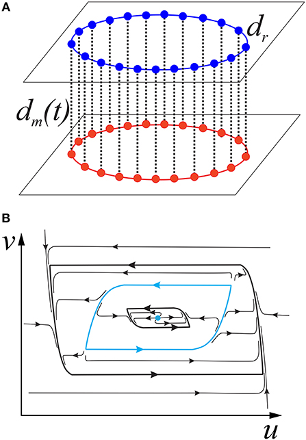
Figure 1. (A) Topology of multiplex network. Red and blue dots depict correspondingly oscillators of first and second layer. Solid and doted lines depict correspondingly intra-layer and (multiplex) inter-layer couplings. (B) Qulitative phase portrait of a single oscillator. There exist two stable limit cycles (bold black lines) separated by an unstable limit cycle (bold blue line) and an unstable equilibrium state (bold blue dot) located at the origin.

If the oscillators do not interact with each other, i.e., d_r = 0; d_m(t) ≡ 0, then the dynamics of each oscillator is described by second-order equation. Two stable limit cycles with “low” and “high” amplitudes exist on the (u, v) phase plane (see Figure 1B). The regions of attraction of these cycles are separated by an unstable limit cycle. An unstable equilibrium state is located at the coordinate origin (u = 0, v = 0). Thus, an oscillator can be either in the regime of low-amplitude oscillations with a dimensionless frequency of 0.0039 or, in the case of initial conditions “outside” the unstable cycle, in the regime of high-amplitude oscillations with a dimensionless frequency of 0.0021.

In our previous paper [32] we showed that various chimera states exist in a separate layer of system (1) at the chosen parameters and obtained chimera states at the experimental system consisting of seven bistable self-exciting oscillators with linear couplings. The example of chimera state is presented in Figure 2A by black crosses (distribution of instant phases φ, average amplitudes < A >, and average frequencies < ω >). Coherent part of the chimera state is formed by first 99 (j = 1 − 99) oscillators with high-amplitude oscillations, and incoherent part is formed by oscillators with j = 101 − 199 that demonstrate alternately the low- and high-amplitude oscillations. The oscillation frequencies and phases of oscillators were calculated as follows. For definiteness, we consider the jth oscillator in the ith layer. Let ${t_{j}^{n}}$ be a sequence of time instants at which the output voltage of the oscillator increases and intersects the straight line $u_{j}^{i} = 0$ ; i.e.,

t_{j}^{n} = {t : u_{j}^{i} (t) = 0, v_{j}^{i} (t) > 0} .

Then, the oscillation phase of the jth oscillator at the time t is given by the expression

\begin{array}{l} ϕ_{j} = 2 π ω_{j}^{n} (t - t_{j}^{n}) for t \in [t_{j}^{n}, t_{j}^{n + 1}], & (2) \end{array}

and $ω_{j}^{n} = \frac{1}{t_{j}^{n} - t_{j}^{n - 1}}$ is the instantaneous oscillation frequency. This definition of the phase is meaningful only if $w_{j}^{n}$ are constant or quite close to each other. In the former case, the oscillator undergoes regular oscillations and the phase always varies at the same rate. In the latter case, oscillations can be, in particular, irregular and the phase is a piecewise linear function of the time. Furthermore, the phase introduced in Equation (2) describes the dynamics of only an individual oscillator decoupled from the remaining system. For this reason, to describe the dynamics of the system as a whole, it is more convenient to use the parameter $φ_{j}^{k} = ϕ_{j} - ϕ_{k}$ describing the oscillation phase of the jth oscillator with respect to oscillations of the reference kth oscillator. If $φ_{j}^{k}$ is independent of time, this means the phase matching of oscillations of the kth and jth oscillators. In the general case of interaction between oscillators, instantaneous frequencies and amplitudes are not constant. For this reason, here and below, frequencies and amplitudes are calculated with averaging over a quite long time series

< ω_{j} > = \frac{1}{n} Σ_{n} ω_{j}^{n}

and

< A_{j} > = \frac{1}{n} Σ_{n} A_{j}^{n},

where $A_{j}^{n} = {v_{j}^{i} (t) : u_{j}^{i} (t) = 0, v_{j}^{i} (t) > 0}$ .

FIGURE 2

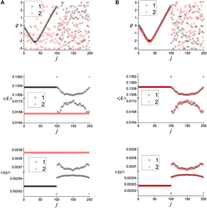
Figure 2. Cloning of chimera state in system (1). Distribution of instant phases φ, average amplitudes < A > and average frequencies < ω > (from up to bottom) at the initial instant of time (A); after the interaction (B). Indexes “1” (black cross) and “2” (red circle) correspond respectively to the first and second layer states. Parameters values: a = 0.32, b = 0.79, c = 1.166, ε = 0.001, d_r = 0.006, d = 0.06, T_c = 1, 000, and N = 200.

Notice that in addition to the coherent and incoherent parts, the chimera state also contains two isolated oscillators at j = 100 and j = 200. Such solitary states exist due to the bistability of the network oscillators. The explanation of this phenomenon was given in Nekorkin et al. [46]. The bistability leads to formation of amplitude clusters with high- and low-amplitude oscillations and so to an amplitude gap (see the amplitude distribution in Figure 2A). The amplitude gap, in turn, causes a frequency gap. Since the magnitudes of gaps are quite large, diffusive coupling between the oscillators leads to emergence of solitary oscillators whose dynamics “smooths out” the dynamics of clusters (amplitude and frequency) having significantly different characteristics.

3. Cloning of Chimera States

Let the chimera state exist in the first layer at the initial instant of time when there is no interaction between the layers (black crosses in Figure 2A). And the initial conditions in the second layer correspond to the low-amplitude oscillations with random initial phases (red circles in Figure 2A). Now if we switch on the interaction between the layers, and then after some time switch the interaction off, then we can obtain a clone of the initial chimera state in the second layer. For certain values of strength and time of multiplex interaction, in the second layer, a chimera state is formed with the same average frequency and amplitude distributions in coherent and incoherent parts, as well as an identical phase distribution in coherent part, as in the chimera which was set in first layer. The example of such cloning for interaction strength d = 0.06 and interaction time T_c = 1, 000 is shown in Figure 2. Notice that, by definition, instantaneous phases of the incoherent parts in the chimera state should be random, and integral characteristics, e.g., average frequencies and amplitudes, are of fundamental importance for the incoherent part. For this reason, we believe that the coincidence of the phases of the incoherent parts is not necessary for the cloning of chimera states. Note that the cloning of chimera states occurs with certain initial conditions The role of initial conditions in more detail is discussed in section 4.

Next we show that the cloning effect is structurally stable. To do this, we introduce a reference layer with the index “0." Let us set in the reference layer a chimera state with the same characteristics as the original chimera that we set in the first layer. Then after the interaction of the first and the second layers we compare states formed in those layers with one in the reference layer using the following characteristics:

\begin{array}{l} ω_{e r r}^{i} = \max_{1 \leq j \leq N} | \frac{< ω_{i, j} > - < ω_{0, j} >}{< ω_{0, j} >} |, \\ A_{e r r}^{i} = \max_{1 \leq j \leq N} | \frac{< A_{i, j} > - < A_{0, j} >}{< A_{0, j} >} | \end{array}

where < ω_i,j > and < A_i,j > are averaged frequencies and amplitudes of the oscillators with the number j of the ith layer; accordingly, < ω_0,j > and < A_0,j > are those in the reference layer.

The results of such calculations for T_c = 1, 000 are presented in Figure 3. They indicate that there is an interval of multiplex coupling strength 0.37 ≤ d ≤ 0.96 where the states in all layers have the same averaged characteristics as the reference chimera state. Thus, the cloning occurs in the large enough interval of strength and so the effect is structurally stable.

FIGURE 3

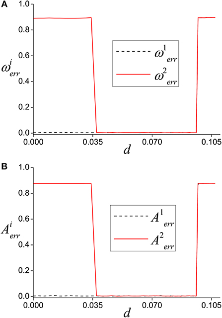
Figure 3. Dependence of the maximum errors between the average frequencies $ω_{e r r}^{i}$ (A) and amplitudes $A_{e r r}^{i}$ (B) in the reference chimera state and the states occurring in first (dashed line) and second (solid line) layer. Parameters values: a = 0.32, b = 0.79, c = 1.166, ε = 0.001, d_r = 0.006, and T_c = 1, 000.

4. The Cloning Mechanism

We showed above that cloning of chimera states takes place when strength of coupling between the elements of the same layer is much smaller than that between the elements of different layers (d_r < < d, see Figure 3). So in the first approximation we can assume that the key role in cloning is played by the dynamics of (multiplex) pairs of elements taken from different layers. Next we consider the dynamics of a pair in more detail. It is described by the following system of equations:

\begin{array}{l} \begin{array}{l} ε \frac{d u_{1}}{d t} = f (u_{1}) - v_{1} + d_{m} (t) (u_{2} - u_{1}) \\ ε \frac{d u_{2}}{d t} = f (u_{2}) - v_{2} + d_{m} (t) (u_{1} - u_{2}) \\ \frac{d v_{1}}{d t} = u_{1}, \\ \frac{d v_{2}}{d t} = u_{2}, \end{array} & (3) \end{array}

where $u_{1} \equiv u_{j}^{1}$ , $u_{2} \equiv u_{j}^{2}$ , $v_{1} \equiv v_{j}^{1}$ , $v_{2} \equiv v_{j}^{2}$ .

Notice also that to realize the cloning, initial conditions in non-interacting layers must be formed in a special way. In particular, a chimera state is set in the first layer with coherent part formed by the oscillators, demonstrating high-amplitude oscillations, and incoherent part formed by the oscillators demonstrating alternately low- and high-amplitude oscillations. In the second layer all oscillators are set in the regime of low-amplitude oscillations whose phases are randomly distributed. Moreover, after interaction, the elements of the second layer should switch to the regimes the corresponding elements of the first layer were in initial moment. Thus, we need to consider the evolution of a pair only for two types of initial conditions:

(I.C.)₁ An oscillator of the first layer is in the regime of high-amplitude oscillations, while that of the second layer is in the regime of low-amplitude oscillations;

(I.C.)₂ The oscillators of both layers are in the regime of low-amplitude oscillations.

4.1. Dynamics of a Pair of Constantly Coupled Oscillators

First, we study dynamics of a pair for the case when interaction between its oscillators is not limited by time. Then we obtain the following system of equations:

\begin{array}{l} \begin{array}{l} ε \frac{d u_{1}}{d t} = f (u_{1}) - v_{1} + d (u_{2} - u_{1}) \\ ε \frac{d u_{2}}{d t} = f (u_{2}) - v_{2} + d (u_{1} - u_{2}) \\ \frac{d v_{1}}{d t} = u_{1}, \\ \frac{d v_{2}}{d t} = u_{2}, \end{array} & (4) \end{array}

Since 0 < ε ≪ 1, the system (4) belongs to the class of fast-slow systems. Such systems are characterized by the presence of two timescales (or speeds), namely, fast and slow ones. In the result, the trajectories of the systems have epochs of a slow and a fast movements. In our system u₁ and u₂ are fast variables, while v₁ and v₂ are slow variables. Next to study the dynamics of the system we use GPST theory. According to the GPST, the partition of phase space ℝ⁴ of system (4) into trajectories can be established by studying two subsystems. As ε → 0, the trajectories of system (4) converge during fast epochs to the trajectories of the fast subsystem (or layer equations)

\begin{array}{l} \begin{array}{l} \frac{d u_{1}}{d τ} = f (u_{1}) - v_{1} + d (u_{2} - u_{1}) \\ \frac{d u_{2}}{d τ} = f (u_{2}) - v_{2} + d (u_{1} - u_{2}) \\ \frac{d v_{1}}{d τ} = 0, \\ \frac{d v_{2}}{d τ} = 0, \end{array} & (5) \end{array}

where t = ετ. During slow epochs the trajectories of (4) converge to the trajectories of the reduced system (or the slow flow)

\begin{array}{l} \begin{array}{l} 0 = f (u_{1}) - v_{1} + d (u_{2} - u_{1}) \\ 0 = f (u_{2}) - v_{2} + d (u_{1} - u_{2}) \\ \frac{d v_{1}}{d t} = u_{1}, \\ \frac{d v_{2}}{d t} = u_{2}, \end{array} & (6) \end{array}

The goal of GPST is to use the fast and slow subsystems (5) and (6) to understand the dynamics of the full system (4) for 0 < ε ≪ 1.

4.1.1. Dynamics of the Fast Subsystem

From system (5) one can see that v₁ = const and v₂ = const, so they play the role of additional parameters (denote them by $v_{1}^{0}$ and $v_{2}^{0}$ correspondingly). Thus, system (5) can be rewritten in the following gradient form

\begin{array}{l} \begin{array}{l} \frac{d u_{1}}{d τ} = - \frac{\partial G}{\partial u_{1}} \\ \frac{d u_{2}}{d τ} = - \frac{\partial G}{\partial u_{2}} \end{array} & (7) \end{array}

where

G = - \int_{0}^{u_{1}} f (x) d x - \int_{0}^{u_{2}} f (x) d x + v_{1}^{0} u_{1} + v_{2}^{0} u_{2} + \frac{d}{2} {(u_{1} - u_{2})}^{2} .

Since

\frac{d G}{d τ} = - {(\frac{\partial G}{\partial u_{1}})}^{2} - {(\frac{\partial G}{\partial u_{2}})}^{2},

the trajectories of system (7) [and so system (5)], except for equilibrium states, relax to one of the stable equilibrium states. Moreover, since the system is gradient their trajectories relax to the equilibrium states by the fastest way. The number and type of equilibrium states depend on the parameters and may change due to saddle-node bifurcations. For example, for $v_{1}^{0} = v_{2}^{0} = d = 0$ there are 49 equilibrium states, among which there are 16 stable and 9 unstable nodes and 24 saddles. The qualitative phase plane of system (7) in this case is shown in Figure 4.

FIGURE 4

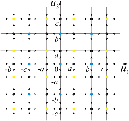
Figure 4. Qualitative phase portrait of fast subsystem (7) for $v_{1}^{0} = v_{2}^{0} = d = 0$ , a = 0.32, b = 0.79, and c = 1.166. The dots mark unstable nodes (blue), stable nodes (yellow), and saddles (black). The lines mark the separatrices of the saddle equilibrium states.

4.1.2. Dynamics of the Reduced Subsystem

The first two algebraic equations in system (6) define a critical manifold $S {(u_{1}, u_{2}, v_{1}, v_{2}) \in ℝ^{4} | f (u_{i}) - v_{i} + d (u_{i + 1} - u_{i}) = 0, i = 1, 2, u_{3} \equiv u_{1}}$ . Let us rewrite (6) in terms of the fast variables u₁ and u₂ to obtain the slow flow on S. For this, we differentiate algebraic Equation (6) with respect to t and combine the result with the equations for ${\overset{\cdot}{v}}_{1}$ and ${\overset{\cdot}{v}}_{2}$ :

\begin{array}{l} (\frac{d f (u_{1})}{d u_{1}} - d) \frac{d u_{1}}{d t} + d \frac{d u_{2}}{d t} = u_{1} \\ (\frac{d f (u_{2})}{d u_{2}} - d) \frac{d u_{2}}{d t} + d \frac{d u_{1}}{d t} = u_{2} & (8) \end{array}

System (8) is a system of linear inhomogeneous algebraic equations for derivatives $\frac{d u_{1}}{d t}$ and $\frac{d u_{2}}{d t}$ . Determinant of its coefficient matrix

Δ = \frac{d f (u_{1})}{d u_{1}} \frac{d f (u_{2})}{d u_{2}} - d (\frac{d f (u_{1})}{d u_{1}} + \frac{d f (u_{2})}{d u_{2}}) .

If Δ ≠ 0, then system (8) has the only solution

\begin{array}{l} \frac{d u_{1}}{d t} = \frac{1}{Δ} [\frac{d f (u_{2})}{d u_{2}} u_{1} - d u_{1} - d u_{2}] \\ \frac{d u_{2}}{d t} = \frac{1}{Δ} [\frac{d f (u_{1})}{d u_{1}} u_{2} - d u_{1} - d u_{2}] . & (9) \end{array}

Note that in the four-dimensional phase space ℝ⁴ of system (4), algebraic equation Δ = 0 and two algebraic equations of system (6) define set $S^{Δ} = \cup_{j} S_{j}^{Δ}$ . Any its element, $S_{j}^{Δ}$ , defines a curve, where the fast and slow trajectories are stitched. According to GPST, each equilibrium state of fast subsystem (5) [and so (7)] in the phase space ℝ⁴ of system (4) corresponds to a submanifold, whose stability with respect to the trajectories of the fast subsystem coincides with the stability of the corresponding equilibrium state. Since the coordinates of the equilibrium states of system (5) depend on two parameters $v_{1}^{0}$ and $v_{2}^{0}$ , any such equilibrium state corresponds to a two-dimensional submanifold in the phase space of (4). The boundary of the submanifold is given by one of the curves $S_{j}^{Δ}$ . Hence the curves $S_{j}^{Δ}$ decompose the critical manifold S into some number of submanifolds of different stability

S = S_{i}^{a} \cup S_{l}^{Δ} \cup S_{k}^{r} \cup S_{j}^{Δ} \cup S_{n}^{s a d},

where $S_{i}^{a}$ denotes one of the stable submanifolds, $S_{k}^{r}$ are the unstable submanifolds, and $S_{n}^{s a d}$ are the saddle submanifolds of the slow flow. Note that Δ > 0 on submanifolds $S_{i}^{a}$ and $S_{k}^{r}$ , Δ < 0 on submanifolds $S_{n}^{s a d}$ and Δ = 0 on submanifolds $S_{l}^{Δ}$ . The number of these submanifolds depends on the parameter d. For example, Figure 5A for d = 0.06 on the phase plane (u₁, u₂) depicts submanifolds $S_{i}^{a}, i = \bar{1, 16}$ , corresponding to stable nodes $O_{j}^{a}$ of the fast subsystem and curves $S_{l}^{Δ}$ .

FIGURE 5

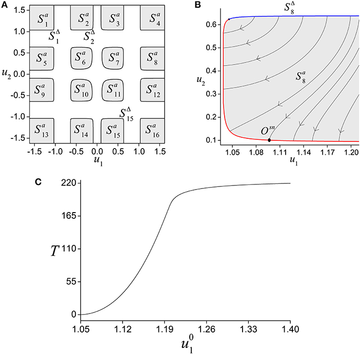
Figure 5. (A) Mutual location of the stable slow submanifolds ( $S_{j}^{a}$ ) of system (5) on the phase plane (u₁, u₂). The boundaries of stable submanifolds ( $S_{j}^{Δ}$ ) defined by the equations Δ = 0. (B) Trajectories behavior on slow submanifold $S_{8}^{a}$ . (C) Dependence of motion time over submanifold $S_{8}^{a}$ to its boundary $S_{8}^{Δ}$ on the initial conditions. Parameter values: a = 0.32, b = 0.79, c = 1.166, and d = 0.06.

Since the system (4) on submanifolds $S_{i}^{a}$ has no equilibrium states and limit cycles, any trajectory starting on the submanifolds eventually leave them. For example, Figure 5B shows the behavior of trajectories on $S_{8}^{a}$ starting on entering part of its boundary $S_{8}^{Δ}$ (blue line) and going till the exit part of the boundary (red line). Note that, the time the trajectories stay on $S_{i}^{a}$ varies depending on the initial conditions. The dependence for trajectories on $S_{8}^{a}$ is shown in Figure 5C. Note that the dependence is a monotonically increasing function asymptotically tending to the value T ≈ 220.

4.1.3. Dynamics of System (4) for Initial Conditions (I.C.)₁

Let us study the dynamics of system (4) for initial conditions (I.C.)₁. Note, the dynamics of system (4) is formed by the alternating dynamics of fast and slow epochs, which results in a “stitched” trajectory.

4.1.3.1. Slow epoch of motion

The initial conditions (I.C.)₁ corresponds to one of the stable submanifolds of slow motions $S_{5}^{a}, S_{8}^{a}, S_{9}^{a}, S_{12}^{a}$ (see Figure 5A). First let the initial conditions belong to $S_{8}^{a}$ . The motions on $S_{8}^{a}$ are defined by system (9). Since Δ > 0 on $S_{8}^{a}$ , we can de-singularize the slow flow near $S_{8}^{Δ}$ by rescaling time with the factor Δ. This gives the following system:

\begin{array}{l} \begin{array}{l} \frac{d u_{1}}{d t_{n}} = \frac{d f (u_{2})}{d u_{2}} u_{1} - d (u_{1} + u_{2}) \\ \frac{d u_{2}}{d t_{n}} = \frac{d f (u_{1})}{d u_{1}} u_{2} - d (u_{1} + u_{2}), \end{array} & (10) \end{array}

where dt = Δdt_n. System (6), and hence system (10), have the only equilibrium point at the origin. Therefore, the trajectories starting on $S_{8}^{a}$ leave the submanifold at some points of its boundary $S_{8}^{Δ}$ . Let $O^{s n} (u_{1} = u_{1}^{0}, u_{2} = u_{2}^{0}) \in S_{8}^{Δ}$ be one of such exit points (see Figure 5B). Since the fast and slow trajectories of system (4) are glued together on $S_{8}^{Δ}$ , the point O^sn is also the equilibrium state of the fast system (5). From this condition we find

\begin{array}{l} \begin{array}{l} v_{1} = f (u_{1}^{0}) + d (u_{2}^{0} - u_{1}^{0}) \\ v_{2} = f (u_{2}^{0}) + d (u_{1}^{0} - u_{2}^{0}) . \end{array} & (11) \end{array}

By using Equation (11) fast system (5) can be rewritten in the form

\begin{array}{l} \begin{array}{l} \frac{d u_{1}}{d τ} = f (u_{1}) - f (u_{1}^{0}) + d (u_{2} - u_{2}^{0} - u_{1} + u_{1}^{0}) \\ \frac{d u_{2}}{d τ} = f (u_{2}) - f (u_{2}^{0}) + d (u_{1} - u_{1}^{0} - u_{2} + u_{2}^{0}) \end{array} & (12) \end{array}

The eigenvalues of the Jacobian matrix of (12) in the point O^sn are given by

\begin{array}{l} λ_{1} = 0, λ_{2} = - 2 d + \frac{d f (u_{1})}{d u_{1}} |_{u_{1} = u_{1}^{0}} + \frac{d f (u_{2})}{d u_{2}} |_{u_{2} = u_{2}^{0}} < 0 & (13) \end{array}

Because of Equation (13), the point O^sn is a saddle-node with an unstable separatrix and a stable nodal branch. Further we show that there are such values of the parameter d that the separatrix W^u(O^sn) tends to the stable node $O_{13}^{a}$ as t → +∞.

4.1.3.2. Fast epoch of motion

Consider the level curves of the function G(u₁, u₂) = C = const, satisfying the condition C ≤ C^sn, where $C^{s n} = G (u_{1}^{0}, u_{2}^{0})$ . Obviously, the curves of the level ${G (u_{1}, u_{2}) = C^{s n}}$ pass through the saddle-node O^sn. In Figure 6A, the curve of this level has a maximum value, i.e., the curves of the higher levels are not indicated (white color), and the curves of the level corresponding to the values of the lower levels (C < C^sn) are marked with different colors. Each color corresponds to the same value of C. Solid black lines in Figure 6 show the critical lines

\begin{array}{l} L_{m i n}^{h} = {(u_{1}, u_{2}) \in R^{2} | - f (u_{2}) + d u_{2} - d u_{1} + f (u_{2}^{0}) \\ + d (u_{1}^{0} - u_{2}^{0}) = 0, - f^{'} (u_{2}) + d > 0} \\ L_{m a x}^{h} = {(u_{1}, u_{2}) \in R^{2} | - f (u_{2}) - d u_{2} + d u_{1} + f (u_{2}^{0}) \\ + d (u_{1}^{0} - u_{2}^{0}) = 0, - f^{'} (u_{2}) + d < 0} \\ L_{m i n}^{v} = {(u_{1}, u_{2}) \in R^{2} | - f (u_{1}) + d u_{1} - d u_{2} + f (u_{1}^{0}) \\ + d (u_{2}^{0} - u_{1}^{0}) = 0, - f^{'} (u_{1}) + d > 0} \\ L_{m a x}^{v} = {(u_{1}, u_{2}) \in R^{2} | - f (u_{1}) + d u_{1} - d u_{2} + f (u_{1}^{0}) \\ + d (u_{2}^{0} - u_{1}^{0}) = 0, - f^{'} (u_{1}) + d < 0} . & (14) \end{array}

At the points of these lines the following conditions are satisfied:

\begin{array}{l} \frac{\partial G}{\partial u_{2}} = 0, \frac{\partial^{2} G}{\partial u_{2}^{2}} > 0, if (u_{1}, u_{2}) \in L_{m i n}^{h} \\ \frac{\partial G}{\partial u_{2}} = 0, \frac{\partial^{2} G}{\partial u_{2}^{2}} < 0, if (u_{1}, u_{2}) \in L_{m a x}^{h} \\ \frac{\partial G}{\partial u_{1}} = 0, \frac{\partial^{2} G}{\partial u_{1}^{2}} > 0, if (u_{1}, u_{2}) \in L_{m i n}^{v} \\ \frac{\partial G}{\partial u_{1}} = 0, \frac{\partial^{2} G}{\partial u_{2}^{1}} < 0, if (u_{1}, u_{2}) \in L_{m a x}^{v} . & (15) \end{array}

Consider the asymptotic behavior of the separatrix of the saddle-node O^sn. Taking into account Equation (8), the location of the level curves of the function ${G (u_{1}, u_{2}) = C^{s n}}$ and lines (14), we establish that for the parameter value d = 0.0075 (Figure 6A) the separatrix W^u(O^sn) asymptotically tends to the equilibrium state $O_{12}^{a}$ . Without changing the coordinates of the point O^sn, we increase the value of the parameter d = 0.0115 (Figure 6B). For this value of the parameter d the lines $L_{m i n}^{h}, L_{m a x}^{v}, L_{m i n}^{v}$ merge at one point, a saddle-node bifurcation of equilibrium states occurs, and a new equilibrium state O* appear (see Figure 6B). With the further increase in the parameter, the equilibrium state O* disappears, and following the arrangement of lines (14) and the level curves of the function G, we find that in this case the separatrix W^u(O^sn) tends to the node $O_{9}^{a}$ (Figure 6C). A further increase in the parameter d leads to the merging of the lines $L_{m i n}^{h}, L_{m a x}^{h}, L_{m i n}^{v}$ (d = 0.020909 = d*). This corresponds to the merging of the node $O_{9}^{a}$ and the saddle O^sad (Figure 6C) and emerging of the saddle-node equilibrium state. For d > d*, this equilibrium state disappears, and the separatrix W^u(O^sn) tends to the equilibrium state $O_{13}^{a}$ (Figure 6D). It is clear that d* depends on the coordinates of the point O^sn.

FIGURE 6

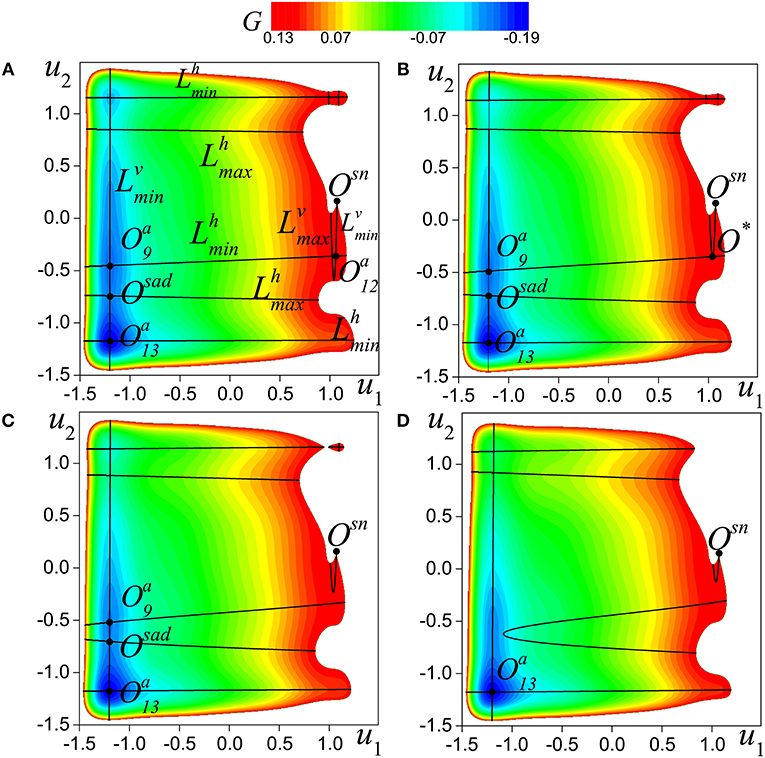
Figure 6. A part of level map of the function G(u₁, u₂) taken at the saddle-node equilibrium state $O^{s n} (u_{1}^{0}, u_{2}^{0})$ of the boundary $S_{8}^{a}$ [i.e., when $v_{1}^{0} = f (u_{1}^{0})$ and $v_{2}^{0} = f (u_{2}^{0})$ ] for (A) d = 0.0075, ( $u_{1}^{0} = 1.07178, u_{2}^{0} = 0.166426$ ); (B) d = 0.0115, ( $u_{1}^{0} = 1.07178, u_{2}^{0} = 0.16196$ ); (C) d = 0.0150, ( $u_{1}^{0} = 1.07178, u_{2}^{0} = 0.15809$ ); (D) d = 0.0225, ( $u_{1}^{0} = 1.07178, u_{2}^{0} = 0.0.14980$ ). Levels depicted are below the one of O^sn (marked by red color). White color marks region with higher levels of G. Curves $L_{m a x}^{h}, L_{m i n}^{h}$ (respectively $L_{m a x}^{v}, L_{m i n}^{v}$ ) defined by Equation (14) are minimum and maximum of G on variable u₂ (respectively variable u₁). O*, O^sad are additional saddle-node equilibrium states and $O_{9}^{a}, O_{12}^{a}$ , and $O_{13}^{a}$ are the node equilibrium states. Parameter values: a = 0.32, b = 0.79, and c = 1.166.

To describe such possible transitions, we introduced the distance R on the plane (u₁, u₂) of system (9) from the origin to $S_{i}^{a}$ . Note that the largest value of R corresponds to the points of the submanifolds $S_{1}^{a}, S_{13}^{a}, S_{4}^{a}$ , and $S_{16}^{a}$ .

Figure 7A depicts the results of analyzing the behavior of the separatrix W^u(O^sn) for different values of $u_{1}^{0}$ belonging to the line of escape $(u_{1}^{0}, u_{2}^{0}) \in S_{8}^{Δ}$ with the submanifold $S_{8}^{a}$ (see Figure 5A). For the values of $u_{1}^{0}, d$ from the region marked by red color, the separatrix W^u(O^sn) of any of the saddle-nodes in the fast system (5) asymptotically tends to the stable node $O_{13}^{a}$ . Since in the phase space ℝ⁴ the equilibrium state corresponds to a stable manifold $S_{13}^{a}$ , high-amplitude oscillations are established in both elements in the system (4). Note that the trajectories of the submanifold $S_{9}^{a}$ of the slow system (10) have a similar behavior. Since the function $\frac{\partial f}{\partial u}$ is even, system (10) does not change when converting (u₁, u₂) → (−u₁, −u₂). Thus, transitions from $S_{9}^{a}$ to $S_{16}^{a}$ exist in ℝ⁴, and high-amplitude oscillations are established in system (4). The initial conditions found by us do not exhaust the entire set of initial conditions under which the oscillation amplitude changes from low to high in the second oscillator.

FIGURE 7

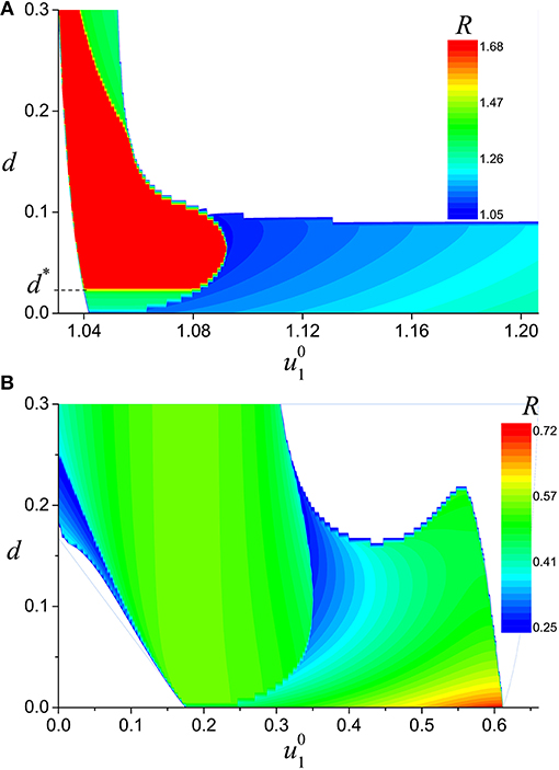
Figure 7. The partition of $(u_{1}^{0}, d)$ - parameter plane into areas corresponding to different transitions [along the trajectories of the fast system (7)] from the border of submanifold (A) $S_{8}^{a}$ (B) $S_{8}^{a}$ . R is the distance from the origin of slow subsystem phase plane (u₁, u₂) to a next stable submanifold. The red color in (A) marks the region where the next manifold is $S_{13}^{a}$ . Non-white colors in (B) mark the region where the next manifold is only one of $S_{6}^{a}$ , $S_{7}^{a}$ , $S_{10}^{a}$ , $S_{11}^{a}$ . Parameters values: a = 0.32, b = 0.79, c = 1.166, and d = 0.06.

4.1.4. Dynamics of System (4) for Initial Conditions (I.C.)₂

Let us study the dynamics of system (4) for initial conditions (I.C.)₂. These conditions correspond to one of the stable submanifolds of slow motions $S_{6}^{a}, S_{7}^{a}, S_{10}^{a}$ , and $S_{11}^{a}$ . Similar to the case of (I.C.)₁ we have analyzed the behavior of the trajectories leaving the submanifolds. Figure 7B depicts the transitions of trajectories starting from the points at the boundary $S_{7}^{Δ}$ of submanifold $S_{7}^{a}$ obtained for different strength of coupling d. One can see that there are no transitions to submanifolds corresponding to high-amplitude oscillations. We have established that such behavior is also typical for other submanifolds, namely $S_{6}^{a}, S_{10}^{a}$ , and $S_{11}^{a}$ .

4.2. Dynamics of a Pair of Short-term Coupled Oscillators

So far, we have considered the dynamics of system (4) without any restrictions on the interaction time. However, in the initial model, the layers interact only during the time T_c. We numerically investigated the dynamics of system (3). For the initial conditions such as (I.C.)₁, Figure 8A shows the behavior of 1, 000 pair of oscillators, or in other words, 1, 000 different initial conditions (I.C.)₁ type, interacting during T_c = 300 and d = 0.06. For all initial conditions, after some transition process, high-amplitude oscillations are established in the interacting pairs. Figure 8B illustrates competition of oscillations in the pairs in the case of initial conditions such as (I.C.)₂ type. Here, interaction of the pairs does not lead to high-amplitude oscillations, and the regime of low-amplitude oscillations persists.

FIGURE 8

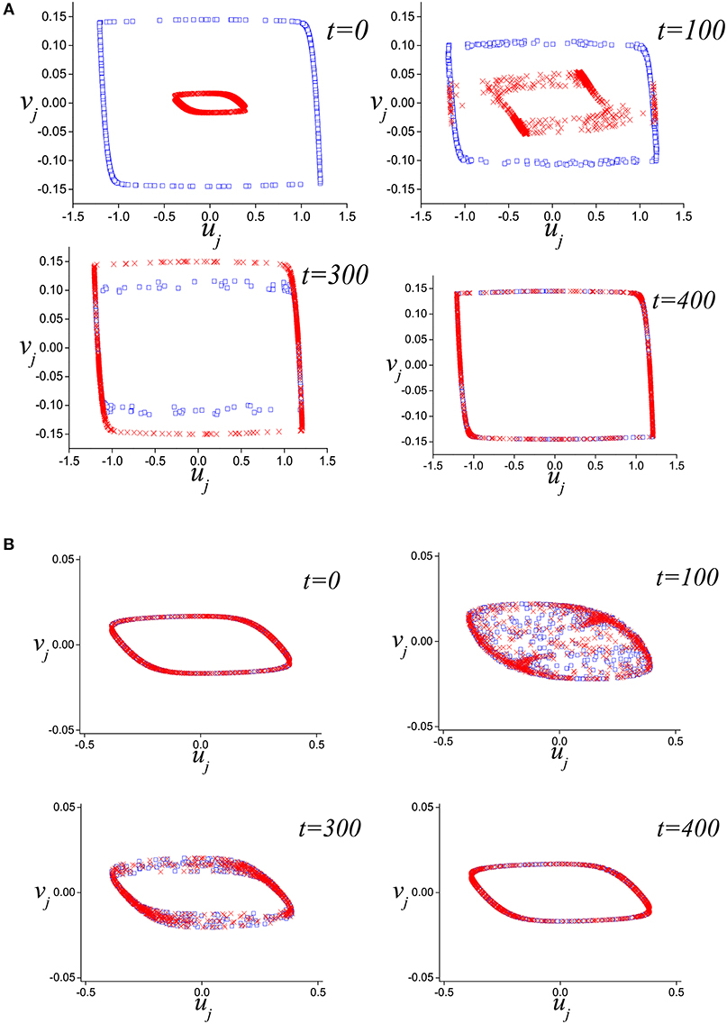
Figure 8. Temporal snapshots of the pair of short-term coupled elements [system (3)] for 1,000 initial conditions such as (A) (I.C.)₁; (B) (I.C.)₂. Parameters values: a = 0.32, b = 0.79, c = 1.166, ε = 0.001, d = 0.06, and T_c = 300.

The occurrence of high-amplitude oscillations for the initial conditions (I.C.)₁ depends on the values of the parameters T_c and d. We examine this dependence numerically and the results are presented in Figure 9. The color gradation on the plane (d, T_c) shows the dependence of the probability of establishing high-amplitude oscillations. The area highlighted in black corresponds to the establishment of high-amplitude oscillations from any initial conditions. The area highlighted in shades of gray corresponds to the establishment of high-amplitude oscillations from only some initial conditions. And finally the area marked in white corresponds to those values of the parameters for which high-amplitude oscillations are not established at all. Note that there are threshold values for both parameters d and T_c. The existence of threshold value for d has already been discussed above. The presence of threshold value for T_c is associated with the motion time T over stable submanifolds (see Figure 6C). Note that the value of the critical value T_c is determined by the dynamics of both oscillators and it is not related to the periods of high and low oscillations of the isolated oscillator.

FIGURE 9

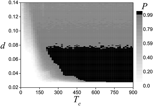
Figure 9. Dependence of establishing probability of high-amplitude oscillations in the pair of short-term coupled elements [system (3)] for initial conditions such as (I.C.)₁ on the parameters (d, T_c). Parameters values: a = 0.32, b = 0.79, c = 1.166, and ε = 0.001.

4.3. Dynamics of the Multiplex Network

Thus, it has been established that in the case of initial conditions (I.C.)₁, there are values of the parameters d and T_c corresponding to the emergence of high-amplitude oscillations in the pairs of interacting oscillators belonging to the different layers. On the other hand, it has been shown that in the case of initial conditions (I.C.)₂, when the oscillators belonging to the different layers do not change their initial regimes after the interaction and keep demonstrating low-amplitude oscillations.

Now let us consider the dynamics of multiplex network (1) based on the findings of the previous subsections. It can be divided into two main stages.

(a) In the time interval 0 < t < T_c, oscillators of different layers interact with each other through inter-layer couplings with strengths, d_c, greatly exceeding those of the diffusive intra-layer couplings, d_r. Therefore, in this stage the main contribution to the dynamics of the system due to the dynamics of the interacting pairs. We have established that as a result of this dynamics, the pairs of oscillators with high-amplitude oscillations are formed in (1) from the initial conditions (I.C.)₁. On the other hand, the pairs of oscillators with low-amplitude oscillations are formed in (1) from the initial conditions (I.C.)₂. This means that the average amplitude distribution in the first layer does not change, while that of the second layer becomes the same as in the first one.

(b) For t > T_c, there are no inter-layer couplings, and the oscillators interact only through diffusive intra-layer ones. Under the influence of these couplings, the neighboring oscillators with similar amplitudes become phase-locked with each other at some average frequency and form the coherent part of the chimera state. The neighboring oscillators with different amplitudes do not become phase-locked with other oscillators and form the incoherent part of the chimera state with distinguished bell-shaped distributions of average frequencies and amplitudes. Thus, the same chimera state is formed in the second layer as in the first one. Note that a finite interaction time is required to stop the competition of oscillations of pairs of oscillators. Otherwise, new complex states arise in the layers and they differ from the initial chimera.

5. Conclusions

In a large two-layer multiplex network with short-term couplings, a new phenomenon of the chimera states cloning, has been discovered and studied. Each layer of the system has a ring topology and consists of relaxation oscillators having two stable limit cycles on their phase planes. The oscillators inside the layers interact through diffusive couplings, while those of different layers interact by means of multiplex couplings. When the chimera state existing in one of the layers interacts for a while with oscillations of the other layer having a random distribution of phases, the same chimera state appears in the latter layer. Note that the time of occurrence of the chimera state in the second layer is less than the minimal partial oscillation period. We have found that the phenomenon is not related with synchronization of oscillations existing in the layers, but instead is determined by the competition of high- and low-amplitude oscillations. Using GPST, we showed that competition of oscillations in each (multiplex) pair of oscillators in the multiplex network is controlled by switching four-dimensional slow-fast dynamics. We have analytically established the initial conditions leading to the trajectories in phase space which start from stable “competitive” submanifolds of slow motions and then transit to stable “winner” submanifolds. The “competitive” submanifold corresponds to the case where oscillations in different layers have different (low and high) oscillation amplitudes. The “winner” submanifold corresponds to the case where oscillations in different layers have high amplitudes. Transitions between stable submanifolds occur along the trajectories of a two-dimensional fast subsystem. The given initial conditions belong to the basin of attraction of both the initial chimera state and the clone. We found that strength, as well as time of multiplex interaction, play a crucial role in the existence of the cloning effect of chimera states. A chimera clone is formed with 100% probability if the strength and time of multiplex interaction exceed certain threshold values. Below these threshold values a chimera clone occurs with a certain probability. Note that the effect of chimera state cloning does not depend on the choice of boundary conditions, since the dynamics of pairs of oscillators plays a crucial role in its existence. We hope also that the cloning effect is not specific to considered model and exists in other models, since the conditions necessary for it to take place are fairly general.

Author Contributions

VN and AD conceived the original ideas. VN supervised the project. AD performed the numerical computations. VN, AD, and DS wrote the manuscript.

Funding

This work was supported by the Russian Foundation for Basic Research (Project Nos. 18-29-10040 and 18-02-00406).

Conflict of Interest Statement

The authors declare that the research was conducted in the absence of any commercial or financial relationships that could be construed as a potential conflict of interest.

References

1. Kuramoto Y. Reduction methods applied to non-locally coupled oscillator systems. In: Hogan J, Champneys A, Krauskopf B, Bernardo M, Wilson E, Osinga H, et al., editors. Nonlinear Dynamics and Chaos: Where Do We Go From Here? Bristol; Philadelphia, PA: Institute of Physics Publishing (2003). p. 209–27.

2. Kuramoto Y, Battogtokh D. Coexistence of Coherence and Incoherence in Nonlocally Coupled Phase Oscillators. Nonlinear Phenomena Complex Syst. (2002) 5:380–5. Available online at: http://www.j-npcs.org/abstracts/vol2002/v5no4/v5no4p380.html

Google Scholar

3. Abrams D, Strogatz S. Chimera states for coupled oscillators. Phys Rev Lett. (2004) 93:174102. doi: 10.1103/PhysRevLett.93.174102

PubMed Abstract | CrossRef Full Text | Google Scholar

4. Abrams D, Mirollo R, Strogatz S, Wiley D. Solvable model for chimera states of coupled oscillators. Phys Rev Lett. (2008) 93:084103. doi: 10.1103/PhysRevLett.101.084103

CrossRef Full Text | Google Scholar

5. Nekorkin V, Voronin M, Velarde M. Clusters in an assembly of globally coupled bistable oscillators. Eur Phys J B Condens Matter Complex Syst. (1999) 9:533–43.

Google Scholar

6. Bordyugov G, Pikovsky A, Rosenblum M. Self-emerging and turbulent chimeras in oscillator chains. Phys Rev E (2010) 82:035205. doi: 10.1103/PhysRevE.82.035205

PubMed Abstract | CrossRef Full Text | Google Scholar

7. Martens EA. Bistable chimera attractors on a triangular network of oscillator populations. Phys Rev E (2010) 82:016216. doi: 10.1103/PhysRevE.82.016216

PubMed Abstract | CrossRef Full Text | Google Scholar

8. Omelchenko I, Maistrenko Y, Hövel P, Schöll E. Loss of coherence in dynamical networks: spatial chaos and chimera states. Phys Rev Lett. (2011) 106:234102. doi: 10.1103/PhysRevLett.106.234102

PubMed Abstract | CrossRef Full Text | Google Scholar

9. Sethia GC, Sen A, Johnston GL. Amplitude-mediated chimera states. Phys Rev E (2013) 88:042917. doi: 10.1103/PhysRevE.88.042917

PubMed Abstract | CrossRef Full Text | Google Scholar

10. Yeldesbay A, Pikovsky A, Rosenblum M. Chimeralike states in an ensemble of globally coupled oscillators. Phys Rev Lett. (2014) 112:144103. doi: 10.1103/PhysRevLett.112.144103

PubMed Abstract | CrossRef Full Text | Google Scholar

11. Zakharova A, Kapeller M, Schöll E. Chimera death: symmetry breaking in dynamical networks. Phys Rev Lett. (2014) 112:154101. doi: 10.1103/PhysRevLett.112.154101

PubMed Abstract | CrossRef Full Text | Google Scholar

12. Laing CR. Chimeras in networks with purely local coupling. Phys Rev E (2015) 92:050904. doi: 10.1103/PhysRevE.92.050904

PubMed Abstract | CrossRef Full Text | Google Scholar

13. Loos SAM, Claussen JC, Schöll E, Zakharova A. Chimera patterns under the impact of noise. Phys Rev E (2016) 93:012209. doi: 10.1103/PhysRevE.93.012209

PubMed Abstract | CrossRef Full Text | Google Scholar

14. Semenova N, Zakharova A, Anishchenko V, Schöll E. Coherence-resonance chimeras in a network of excitable elements. Phys Rev Lett. (2016) 117:014102. doi: 10.1103/PhysRevLett.117.014102

PubMed Abstract | CrossRef Full Text | Google Scholar

15. Schöll E. Synchronization patterns and chimera states in complex networks: interplay of topology and dynamics. Eur Phys J Spec Top. (2016) 225:891–919. doi: 10.1140/epjst/e2016-02646-3

CrossRef Full Text | Google Scholar

16. Semenova NI, Strelkova GI, Anishchenko VS, Zakharova A. Temporal intermittency and the lifetime of chimera states in ensembles of nonlocally coupled chaotic oscillators. Chaos (2017) 27:061102. doi: 10.1063/1.4985143

PubMed Abstract | CrossRef Full Text | Google Scholar

17. Shepelev IA, Vadivasova TE, Bukh AV, Strelkova GI, Anishchenko VS. New type of chimera structures in a ring of bistable FitzHugh–Nagumo oscillators with nonlocal interaction. Phys Lett A (2017) 381:1398–404. doi: 10.1016/j.physleta.2017.02.034

CrossRef Full Text | Google Scholar

18. Maistrenko Y, Brezetsky S, Jaros P, Levchenko R, Kapitaniak T. Smallest chimera states. Phys Rev E (2017) 95:010203. doi: 10.1103/PhysRevE.95.010203

PubMed Abstract | CrossRef Full Text | Google Scholar

19. Martens EA, Thutupalli S, Fourrière A, Hallatschek O. Chimera states in mechanical oscillator networks. Proc Natl Acad Sci USA. (2013) 109:10563–7. doi: 10.1073/pnas.1302880110

CrossRef Full Text | Google Scholar

20. Kapitaniak T, Kuzma P, Wojewoda J, Czolczynski K, Maistrenko Y. Imperfect chimera states for coupled pendula. Sci Rep. (2014) 4:6379. doi: 10.1038/srep06379

PubMed Abstract | CrossRef Full Text | Google Scholar

21. Wojewoda J, Czolczynski K, Maistrenko Y, Kapitaniak T. The smallest chimera state for coupled pendula. Sci. Rep. (2016) 6:34329. doi: 10.1038/srep34329

PubMed Abstract | CrossRef Full Text | Google Scholar

22. Dudkowski D, Grabski J, Wojewoda J, Perlikowski P, Maistrenko Y, Kapitaniak T. Experimental multistable states for small network of coupled pendula. Sci. Rep. (2016) 6:29833. doi: 10.1038/srep29833

PubMed Abstract | CrossRef Full Text | Google Scholar

23. Hagerstrom AM, Murphy TE, Roy R, Hövel P, Omelchenko I, Schöll E. Experimental observation of chimeras in coupled-map lattices. Nat Phys. (2012) 8:658–61. doi: 10.1038/nphys2372

CrossRef Full Text | Google Scholar

24. Larger L, Penkovsky B, Maistrenko Y. Laser chimeras as a paradigm for multistable patterns in complex systems. Nat Commun. (2015) 6:7752. doi: 10.1038/ncomms8752

PubMed Abstract | CrossRef Full Text | Google Scholar

25. Tinsley MR, Nkomo S, Showalter K. Chimera and phase-cluster states in populations of coupled chemical oscillators. Nat Phys. (2012) 8:662–5. doi: 10.1038/nphys2371

CrossRef Full Text | Google Scholar

26. Schmidt L, Schönleber K, Krischer K, García-Morales V. Coexistence of synchrony and incoherence in oscillatory media under nonlinear global coupling. Chaos (2014) 24:013102. doi: 10.1063/1.4858996

PubMed Abstract | CrossRef Full Text | Google Scholar

27. Wickramasinghe M, Kiss IZ. Spatially organized dynamical states in chemical oscillator networks: synchronization, dynamical differentiation, and chimera patterns. PLoS ONE 8:e80586. doi: 10.1371/journal.pone.0080586

PubMed Abstract | CrossRef Full Text

28. Wickramasinghe M, Kiss IZ. Spatially organized partial synchronization through the chimera mechanism in a network of electrochemical reactions. Phys Chem Chem Phys. (2014) 16:18360–9. doi: 10.1039/C4CP02249A

PubMed Abstract | CrossRef Full Text | Google Scholar

29. Smart AG. Exotic chimera dynamics glimpsed in experiments. Phys Today (2012) 65:17–9. doi: 10.1063/PT.3.1738

CrossRef Full Text | Google Scholar

30. Larger L, Penkovsky B, Maistrenko Y. Virtual chimera states for delayed-feedback systems. Phys Rev Lett. (2013) 111:054103. doi: 10.1103/PhysRevLett.111.054103

PubMed Abstract | CrossRef Full Text | Google Scholar

31. Gambuzza LV, Buscarino A, Chessari S, Fortuna L, Meucci R, Frasca M. Experimental investigation of chimera states with quiescent and synchronous domains in coupled electronic oscillators. Phys Rev E (2014) 90:032905. doi: 10.1103/PhysRevE.90.032905

PubMed Abstract | CrossRef Full Text | Google Scholar

32. Shchapin DS, Dmitrichev AS, Nekorkin VI. Chimera states in an ensemble of linearly locally coupled bistable oscillators. JETP Lett. (2017) 106:617–21. doi: 10.1134/S0021364017210111

CrossRef Full Text | Google Scholar

33. Hizanidis J, Lazarides N, Tsironis GP. Robust chimera states in SQUID metamaterials with local interactions. Phys Rev E (2016) 94:032219. doi: 10.1103/PhysRevE.94.032219

PubMed Abstract | CrossRef Full Text | Google Scholar

34. Mukhametov LM, Supin AY, Polyakova IG. Interhemispheric asymmetry of the electroencephalographic sleep patterns in dolphins. Brain Res. (1977) 134:581–4. doi: 10.1016/0006-8993(77)90835-6

PubMed Abstract | CrossRef Full Text | Google Scholar

35. Lyamin OI, Manger PR, Ridgway SH, Mukhametov LM, Siegel JM. Cetacean sleep: an unusual form of mammalian sleep. Neurosci Biobehav Rev. (2008) 32:1451–84. doi: 10.1016/j.neubiorev.2008.05.023

PubMed Abstract | CrossRef Full Text | Google Scholar

36. Andrzejak RG, Ruzzene G, Malvestio I. Generalized synchronization between chimera states. Chaos (2017) 27:053114. doi: 10.1063/1.4983841

PubMed Abstract | CrossRef Full Text | Google Scholar

37. Tian C, Bi H, Zhang X, Guan S, Liu Z. Asymmetric couplings enhance the transition from chimera state to synchronization. Phys Rev E (2017) 96:052209. doi: 10.1103/PhysRevE.96.052209

PubMed Abstract | CrossRef Full Text | Google Scholar

38. Majhi S, Perc M, Ghosh D. Chimera states in a multilayer network of coupled and uncoupled neurons. Chaos (2017) 27:073109. doi: 10.1063/1.4993836

PubMed Abstract | CrossRef Full Text | Google Scholar

39. Kasatkin DV, Nekorkin VI. Synchronization of chimera states in a multiplex system of phase oscillators with adaptive couplings. Chaos (2018) 28:093115. doi: 10.1063/1.5031681

PubMed Abstract | CrossRef Full Text | Google Scholar

40. Hizanidis J, Kouvaris NE, Zamora-López G, Díaz-Guilera A, Antonopoulos CG. Chimera-like states in modular neural networks. Sci Rep. (2016) 6:19845. doi: 10.1038/srep19845

CrossRef Full Text | Google Scholar

41. Ujjwal SR, Punetha N, Ramaswamy R. Phase oscillators in modular networks: the effect of nonlocal coupling. Phys Rev E (2016) 93:012207. doi: 10.1103/PhysRevE.93.012207

PubMed Abstract | CrossRef Full Text | Google Scholar

42. Maksimenko VA, Makarov VV, Bera BK, Ghosh D, Dana SK, Goremyko MV, et al. Excitation and suppression of chimera states by multiplexing. Phys Rev E (2016) 94:052205. doi: 10.1103/PhysRevE.94.052205

PubMed Abstract | CrossRef Full Text | Google Scholar

43. Dmitrichev AS, Shchapin DS, Nekorkin VI. Cloning of chimera states in a multiplex network of two-frequency oscillators with linear local couplings. JETP Lett. (2018) 108:543–47. doi: 10.1134/S0021364018200079

CrossRef Full Text | Google Scholar

44. Fenichel N. Geometric singular perturbation theory for ordinary differential equations. J Different Equat. (1979) 31:53–98. doi: 10.1016/0022-0396(79)90152-9

CrossRef Full Text | Google Scholar

45. Mishchenko EF, Rozov NK. Differntial Equations With Small Parameters and Relaxation Oscillations. New York, NY: Plenum Pres (1980).

46. Nekorkin VI, Makarov VA, Velarde MG. Clustering and phase resetting in a chain of bistable nonisochronous oscillators. Phys Rev E (1998) 58:5742–7. doi: 10.1103/PhysRevE.58.5742

CrossRef Full Text | Google Scholar

Keywords: chimera states, chimera states cloning, dynamical mechanism, bifurcations, relaxation dynamics, multiplex networks

Citation: Dmitrichev A, Shchapin D and Nekorkin V (2019) Cloning of Chimera States in a Large Short-term Coupled Multiplex Network of Relaxation Oscillators. Front. Appl. Math. Stat. 5:9. doi: 10.3389/fams.2019.00009

Received: 30 October 2018; Accepted: 25 January 2019;
Published: 18 February 2019.

Edited by:

Anna Zakharova, Technische Universität Berlin, Germany

Reviewed by:

Jakub Sawicki, Technische Universität Berlin, Germany
Johanne Hizanidis, University of Crete, Greece
Vadim S. Anishchenko, Saratov State University, Russia

Copyright © 2019 Dmitrichev, Shchapin and Nekorkin. This is an open-access article distributed under the terms of the Creative Commons Attribution License (CC BY). The use, distribution or reproduction in other forums is permitted, provided the original author(s) and the copyright owner(s) are credited and that the original publication in this journal is cited, in accordance with accepted academic practice. No use, distribution or reproduction is permitted which does not comply with these terms.

*Correspondence: Aleksei Dmitrichev, admitry@appl.sci-nnov.ru

ORIGINAL RESEARCH article

Cloning of Chimera States in a Large Short-term Coupled Multiplex Network of Relaxation Oscillators

1. Introduction

2. Model of Multiplex Network

3. Cloning of Chimera States

4. The Cloning Mechanism