Data-Driven Modeling and Prediction of Complex Spatio-Temporal Dynamics in Excitable Media

1. Introduction

In life sciences mathematical models based on first principles are scarce and often a variety of approximate models of different complexity exists for describing the given (experimental) dynamical process. For example, electrical excitation waves in cardiac tissue can be described using partial differential equations (PDEs) with 2 to more than 60 variables, covering the range from simple qualitative models [1, 2] to detailed ionic cell models including not only cell membrane voltage but also different ionic currents and gating variables [3, 4]. While there are several modalities for measuring membrane voltage (electrical sensors, fluorescent dyes [5]) it is in general much more difficult and expensive (if not impossible) to directly measure the other variables of the mathematical model, such as ionic currents or gating variables. In such cases it is desirable to (cross) estimate variables, which are difficult to assess from those that can be easily measured. In control theory this task is addressed by constructing an observer based on a given mathematical model describing the process of interest. Once all state variables of the model have been estimated, the model (e.g., a PDE) can be used to simulate and forecast the future evolution of the dynamical process. This combination of cross estimation and prediction of dynamical variables is the core of all data assimilation methods [6–10] where again the model equations are involved and have to be known. In this contribution, we present a machine learning method for estimating all state variables and forecasting their evolution from limited observations. This “black-box model" consists of a convolutional neural network (CNN) combined with a conditional random field (CRF) and will be introduced in section 2. For training and evaluating the network two dimensional spatio-temporal time series are used, which were generated by the Bueno-Orovio-Fenton-Cherry (BOCF) model [11] describing complex electrical excitation waves in cardiac tissue. This model is introduced in section 3. As modeling tasks we consider cross estimation of variables, forecasting dynamics using an iterative feedback scheme, and a combination of forecasting and cross estimation providing future values of not measured variables. These results are presented in section 4. A summary and a brief discussion of potential future developments are given in section 5.

2. Data Driven Modeling

In data driven modeling mathematical models are not based on first principles (e.g., Newton's laws, Maxwell's equations, …) but are directly derived from experimental measurement data or other physical observations. The model should describe the experiment as precisely as possible but it also should possess a high level of generalizability, i.e., the ability to provide a suitable and good description for data from a very similar experiment. Therefore, overfitting has to be avoided and all irrelevant aspects that are not necessary to describe the desired effect should be discarded when generating the model (without employing human expert knowledge). Many approaches for generating (dynamical) models from (training) data have been devised including autoregressive models [12], evolutionary algorithms in particular genetic algorithms [13], local modeling [14], reservoir computing [15–19], symbolic regression [20], or adaptive fuzzy rule-based models [21]. Furthermore, Monte Carlo techniques may be used for assessing uncertainty in model parameters [22]. In this work we present a modeling ansatz which combines deep convolutional neural networks [23] for feature extraction and dimension reduction with conditional random fields (CRFs) [24] for modeling the properties of temporal sequences.

2.1. Artificial Neural Network

Artificial neural networks (ANNs) [25–27] are parameterizable models for approximating a (unknown) function F implicitly given by the data. The actual function provided by the ANN:

should be a good approximation of F, i.e., f ≃ F. Here O ∈ ℕ and P ∈ ℕ denote the dimension of the input and the output of f, respectively. A widely used type of ANN are feed-forward neural networks (FNN) where, in general, f is given by

with a non-linear function ψ applied component-wise, an input vector X ∈ ℝ^O, a weight matrix W ∈ ℝ^P×O, and a bias b ∈ ℝ^P. Equation (2) is called a one-layer FNN. By recursively applying the output of one layer as input to the next layer, a multi-layer FNN can be constructed:

Equation (3) describes a multi-layer FNN with L ∈ ℕ layers. In the following an input with several variables is considered and the input is given by X ∈ ℝ^h×w×d, with h ∈ ℕ rows and w ∈ ℕ columns of the input field, and the number of variables d. To improve the approximation properties of the network Equation (3), FNNs may contain additional convolutional layers leading to state-of-the-art models for data classification, so-called convolutional neural networks (CNNs) [23].

2.2. Network Architecture

The network used in the following for prediction of multivariate time series is built based on the architecture of a convolutional autoencoder [28], with residual connections [29] consisting of an encoding path (left half of the network, from 512 × 512 to 64 × 64) to retrieve the features of interest and a symmetric decoding path (right half of the network, from 64 × 64 back to 512 × 512). As illustrated in Figure 1 each encoding/decoding path consists of multiple levels, i.e., resolutions, for feature extraction on different scales and noise reduction. The conditional random field block has a special role: Based on the selected feature, the CRF should map a sequence of features of a previous time step t to the next time step t + Δt. The other four components of the network are basic building blocks, like regular convolutional layers followed by rectified linear unit activation and batch normalization (these blocks are omitted in Figure 1 for simplicity). Each residual layer consists of three convolutional blocks and a residual skip connection. A maxpooling layer is located between levels in the encoding path to perform downsampling for feature compression. The deconvolutional layer [30] is located between levels in the decoding path to up-sample the input data using learnable interpolations. The input for the network are all four system variables of the BOCF model which will be introduced in section 3.1 or a sequence of the four system variables as introduced in section 4.1. The output of the network always consists of four system variables.

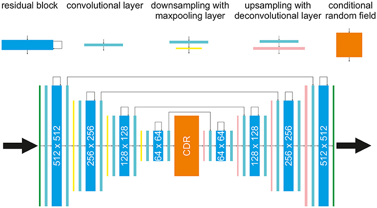
Figure 1. The proposed architecture for forecasting and cross-estimation consisting of a splitted autoencoder and a conditional random field (CRF, orange block) in the middle, with residual blocks (cyan blocks), convolutional layers (turquoise blocks), maxpooling and downsampling layers (yellow blocks), and deconvolutional layers (pink blocks).

2.3. Convolution Layer

Convolutional neural networks [23, 26, 27] receive a training data set ${X}=\left\{X_1,X_2,\dots ,X_m\right\}$, where $X_{\alpha }\in {ℝ}^{h\times w\times d}$. The data processing through the network is described layer-wise i.e., in the l-th convolutional layer the input X^(l) will be transformed to the raw output o^(l), which is in turn the input to the next layer l+1, where the dimension changes depending on the number and size of convolutions, padding and stride of the layers as illustrated in Figure 1. The padding parameter P^(l) ∈ ℕ, for layer l, describes the number of zeros at the edges of a field by which the field is extended. This is necessary since every convolution being larger than 1 × 1 will decrease the output size. The stride parameter S^(l) ∈ ℕ is the parameter determining how much the kernel is shifted in each step to compute the next spatial position (x, y). This specifies the overlap between individual output pixels, and it is here set to 1. Each layer l is specified by its number of kernels K^(l) = {K^{(l, 1)}, K^{(l, 2)}, …K^(l,d(l))}, where d^(l) ∈ ℕ is the number of kernels in layer l, and its additive bias terms b^(l) = {b^{(l, 1)}, b^{(l, 2)}, …, b^(l,d(l))} with b^{(l, d)} ∈ ℝ. Note that the input X^{(l, d)} ∈ ℝ^h(l)×w^(l) in the l-th layer with size h^(l)×w^(l), kernel k, and depth d^(l) is processed by a set of kernels {K^{(l, d)}}. For each kernel $K^{(l,d)}\in {ℝ}^{h_K^{(l)}\times w_K^{(l)}}$ with size $h_K^{(l)}\times w_K^{(l)}$ and d ∈ {1, …, d^(l)}, the raw output $o^{(l)}\in {ℝ}^{\frac{h^{(l)}-h_K^{(l)}-1+P^{(l)}}{S^{(l)}}\times \frac{w^{(l)}-w_K^{(l)}-1+P^{(l)}}{S^{(l)}}}$ is computed element by element as:

The result is clipped by an activation function ψ to obtain the activation $\psi (o_{x,y}^{(l,d)})$ of each unit in layer l:

To obtain o^(l) = {o^{(l, 1)}, …, o^(l,d(l))}, Equation (5) needs to be calculated ∀d = 1, …, d^(l) and ∀(x, y). Each spatial calculation of $o_{x,y}^{(l,d)}$ is considered as a unit and $\psi (o_{x,y}^{(l,d)})$ as the feedforward activation of the unit. The value of an element of a kernel ($K_{i,j}^{(l,d)}$) between two units is the weight of the feedforward connection. Such systems are well-suited for feature extraction [28], but their linear structure does not allow a direct modeling of temporal changes or the possibility to process a sequence of data. To enable temporal modeling, we employ linear-chain conditional random fields [31] that will be introduced in the next section.

2.4. Linear-Chain Conditional Random Fields

To implement a probabilistic forecasting block we consider the output of the convolutional layer o and the corresponding forecast q as random variables O and Q, respectively. Both random variables O and Q are jointly distributed and in a predictive framework we aim at constructing a conditional model P(Q|O) from paired observation and forecast sequences. Let G = (V, E) be a undirected graph such that Q = (Q_{v)v ∈ V}, where Q is indexed by the vertices of G. Each vertex in G represents a state, a history or a forecast. Then (O, Q) is a conditional random field (CRF), if conditioned on O the random variables Q_v obey the Markov property [24]. A linear-chain conditional random field, where o is a sequence of historical extracted features and q a corresponding forecasted feature in the future, is given by:

where $q\in {Q}$, ${Q}$ is a set of future events, $\mathbf{\text{h}}\in {H}$, ${H}$ is the set of layers of the CRF where each element h_i of h represents a historical state of an event at time t. θ is the set of parameters. Ψ(q, h, o; θ) is a so called potential function (also called local or compatibility function) which measures the compatibility (i.e., high probability) between a forecast, a set of observed features, and a configuration of historical states, such that:

Here n is the number of historical states and ϕ_j(o, ω) is a vector that can include any feature of the observation specific for a specific time window ω, and θ = [θ_h, θ_q, θ_ϵ, θ_p] are model parameters. To restrict the search space for possible parametrizations only sine, cosine, and a linear interpolation function are allowed to be used as feature functions. θ_h[h_j] is the parameter that corresponds to the state h_j. The function θ_q[q, h_j] indicates the parameters that corresponds to the forecast q and the state h_j. θ_ϵ[q, h_i, h_k] refers to parameters that describe the dependency relation between the nodes h_i and h_k. θ_p[q] defines the parameters for q given the features over the past, while the dot product ϕ_j(o, ω)·θ_n[h_j] measures the compatibility between the observed features and the state at time j. In contrast to this ϕ(o, ω)·θ_p[q] measures the compatibility between observation and the forecast. h consists of k = 1, 024 elements and the last term in Equation (7) captures the influence of the past features on the forecast. For training the following likelihood function is defined:

where n is the number of training examples. By maximizing the likelihood for the forecasted training data the optimal parameter set θ* is determined. To find θ* Equation (8) can be evaluated by the same gradient descent method which is used for optimizing/training the autoencoder. To forecast the input sequence with a linear-chain CRF it is necessary to compute the q sequence that maximizes the following equation:

The sequence maximizing this is then used by the deconvolutional part of the network to map the features back to the desired system variables at t + Δt.

3. Modeling Excitable Media

Excitable systems are non-linear dynamical systems with a stable fixed point. Small perturbations of the stable equilibrium decay, but stronger perturbations above some characteristic threshold lead to a high amplitude excursion in state space until the trajectory returns to the stable fixed point. In neural or cardiac cells this response leads to a so-called action potential. After such a strong response a so-called refractory period has to pass until the next excitation can be initialized by perturbing the system again. An excitable medium consists of excitable systems (e.g., cells), which are spatially coupled. Electric coupling of neighboring cardiac cells, for example, can be modeled by means of a diffusion term for local currents. The resulting partial differential equations (PDEs) describe the propagation of undamped solitary excitation waves. Due to the refractory time of local excitations spiral or scroll waves are very common and typical hallmarks of excitable media, which can lead to stable periodically rotating wave patterns or may break-up forming complex chaotic wave dynamics. From the large selection of different PDE models describing excitable media we have chosen the Bueno-Orovio-Cherry-Fenton (BOCF) model which was devised as an efficient model for cardiac tissue [11].

3.1. Bueno-Orovio-Cherry-Fenton Model

The Bueno-Orovio-Cherry-Fenton (BOCF) model [11] provides a compact description of excitable cardiac dynamics. We use this model as a benchmark to validate our approach for forecasting and cross-estimation of complex wave patterns in excitable media. The evolution of the four system variables of the BOCF model is given by four PDEs

where u represents the membrane voltage and H(·) denotes the Heaviside function. The three currents J_si, J_fi and J_so are given by the equations

Furthermore, seven voltage dependent variables

are required. The characteristic model dynamics is determined through 28 parameters. In our simulations we used a set of parameters [11] given in Table 1 for which the BOCF model exhibits chaotic excitation wave dynamics similar to the Ten Tusscher-Noble-Noble-Panfilov (TNNP) model [32].

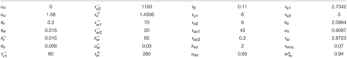
Table 1. TNNP model parameter values for the BOCF model [11].

The spatio-temporal chaotic dynamics of this system is actually transient chaos whose lifetime grows exponentially with system size [33, 34]. To obtain chaotic dynamics with a sufficiently long lifetime the system has been simulated on a domain of 512 × 512 grid points with a grid constant of Δx = 1.0 space units and a diffusion constant D = 0.2. Furthermore, an explicit Euler stepping in time with Δt = 0.1 time units¹, a 5 point approximation of the Laplace operator, and no-flux boundary conditions were used. Figure 2 shows typical snapshots of the dynamics.

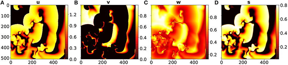
Figure 2. Snapshots from the BOCF model at t = 100 of (A) the u variable, (B) the v variable, (C) the w variable, and (D) the s variable.

4. Results

The proposed network model was trained with simulated data generated by the BOCF model with parameter values given in Table 1. Ten trajectories with different initial conditions for the variables u, v, w, and s were generated by simulating the BOCF model for a time series of 50,000 samples spanning a period of time of 5 s. Five of these data sets randomly chosen, were used to train the network, while the other solutions were used for validation. For training the Adam optimizer [35] was used, with a learning rate lr = 0.0001 and β₁ = 0.9, β₂ = 0.999.

In order to quantify the performance of the estimation and prediction methods the similarity of target fields and output fields of the network has to be quantified. For this purpose we use the Jensen-Shannon divergence (JSD) [36] applied to normalized fields of the variables of the BOCF model. The JSD of two discrete probability distributions A and B is defined as

where $M=\frac{1}{2}(A+B)$ and D_KL(A||M) is the Kullback-Leibler divergence [37]:

During training the JSD was used as objective function to be minimized (for a GPU implementation of the JSD see [38]). The JSD is bounded by 0 and 1 and a value below 0.02 was considered to indicate no discernible differences between the two distributions (fields). An alternative for quantifying the deviation would be the Fractions Brier Score [39]. For training the network, for each trajectory at each time step, sequences of lengths up to m = 10 were used as input.

The input of the network consisted of fields of variables that were assumed to be measured and random fields representing variables that were considered to be not available.

4.1. Forecast

For forecasting the input of the network consisted of sequences of length m = 10 of u, v, w, and s given by {u_t−m+1, …, u_t}, {v_t−m+1, …, v_t}, {w_t−m+1, …, w_t}, and {s_t−m+1, …, s_t}. The desired output of the network is then u_t+Δt, v_t+Δt, w_t+Δt and s_t+Δt. By using the output of the network as a new input the system can be run iteratively in a closed loop for long term prediction. The development of the JSDs of u, v, w, s through time are shown in Figure 3A. Since the u and the s fields look quite similar (see Figures 2A,D) their JSD-values are almost the same. The w-field (Figure 2C) exhibits relatively high values at all spatial locations and therefore the JSD of two such fields is rather low. On the other hand, the v field (Figure 2B) possesses only very localized structures with high values and this leads to rather high values of the JSD for (slightly) different fields. Figure 3B shows for comparison the root normalized mean squared errors (RNMSE) of all variables u, v, w, s which is given by

where

Here $\stackrel{-}{v}$ denotes the temporal and spatial mean values of the BOCF sequence of length T_F, M² = 512·512 is the number of grid points of the domain and $v_{ij}^{\mathrm{\text{BOCF}}}$ denotes the value of variable v at grid point (i, j) for the reference solution generated by the BOCF model. As can be seen in Figure 3A all four curves possess very similar values and indicate an increase of the error already during the initial period for t ∈ [0, 1000].

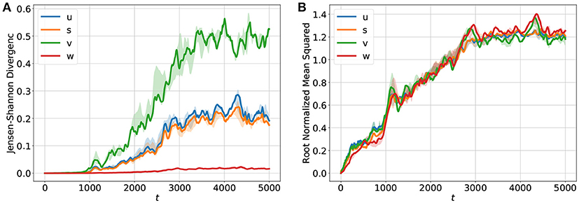
Figure 3. Temporal development of (A) the Jensen-Shannon divergence (JSD) and (B) the root normalized mean squared error (RNMSE) for all variables u, v, w, s showing the deviation of the iterative network prediction (in a feedback mode) from the reference orbit obtained with the BOCF model. During the period [0−1000] the predicted and the true fields agree very well as indicated by very small values of the JSD. In the time interval (1000−3000] the JSD values increase until they saturate and the forecasts become very poor and useless. The RNMSE values show a similar increase in time but turn out to be more sensitive to minor deviations during the initial phase [0−1000] of the forecast. The solid curves show median values of JSD and RNMSE obtained from ten different initial values of u, v, w, s. The transparent areas visualize the 0.25/0.75 percentile.

Figure 4 shows a comparison of the error dynamics of the forecast obtained with the iterated network with feedback (orange curve) and the dynamics of a BOCF model starting from slightly perturbed initial conditions (blue curve). Both curves give the root normalized mean squared error (RNMSE) with respect to the same reference orbit generated by the BOCF model. The perturbation of the initial condition of the second BOCF solution with respect to the initial condition of the reference orbits was chosen to be very small. Therefore, during the initial phase the deviation still remains so small that (with semi-logarithmic axes) a linear segment of the error curve occurs that can be used to estimate the largest Lyapunov exponent [40]. Once the error of the perturbed BOCF orbit (blue curve) reaches the level of the network prediction error (orange curve) both error curves continue to increase in the same way indicating that the network almost perfectly learned the true dynamics of the BOCF model.

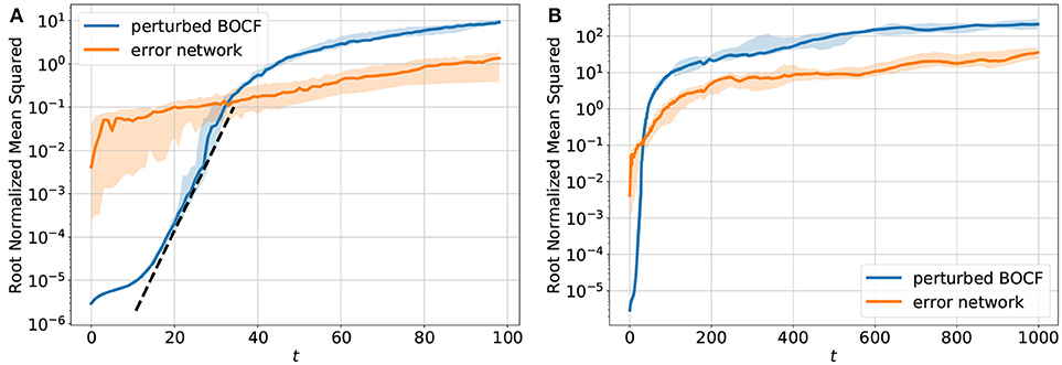
Figure 4. Temporal development of the sum of the root normalized mean squared errors (RNMSE) of all variables u, v, w, s. (A) shows the NMSE for t ∈ [1, 100] and (B) shows the NMSE for t ∈ [1, 1000]. The orange curve describes the deviation of the trajectory generated by the network from the reference orbit simulated with the BOCF model. For comparison the blue curve shows the distance between the reference orbit and a second solution of the BOCF model obtained by perturbing the initial conditions where each variable was perturbed at every spatial location using Gaussian random noise (μ = 0, σ² = 10⁻¹¹). The error dynamics of ten perturbed trajectories was analyzed. These orbits were obtained by perturbing the reference orbit at different times [0, 1000), [1000, 2000), …[9000, 10000). The blue curve shows the median and the 0.25/0.75 percentile is visualized by the transparent areas. The dotted black line (A) denotes the slope the linear part of the log(NMSE) vs. t curve which provides an estimate of the largest Lyapunov exponent [40] λ₁ ≈ 0.25 (with respect to the natural logarithm).

To illustrate the deviation between the u field forecasted by the network and the (true) u field provided by the simulation of the BOCF PDE Figure 5 shows snapshots at times t = 500, t = 1, 500, t = 3, 000, and t = 5, 000. While at t = 500 original (A) and forecast (E) are almost indistinguishable the snapshots at t = 1, 500 exhibit minor differences (Figures 5B,F). At time t = 3, 000 only rough structures agree (Figures 5C,G) until at t = 5, 000 forecast and simulation appear completely decorrelated (Figures 5D,H). The full evolution of the forecast compared to the original dynamics generated with the BOCF model is also available as a movie (Supplemental Data). Compared to a typical spiral rotation period of approximately T_sp = 350 good forecasting results can be obtained for about five spiral rotations corresponding to 5*350 / 4 = 437 Lyapunov times T_L = 1/λ₁ ≈ 4 given by the largest Lyapunov exponent λ₁ ≈ 0.25 (see Figure 4).

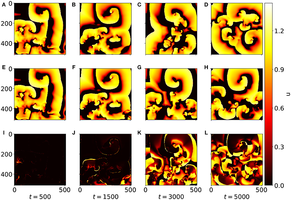
Figure 5. Snapshots of u at different time steps. (A–D) Show the (reference) values from the BOCF simulation, while (E–H) display the values forcasted by the network. The diagrams (I–L) show the absolute deviation of the forecasted values from the reference values. At t = 500 the patterns (A,E) are still (almost) indistinguishable, and for t = 1, 500 still only minor differences between (B,F) are noticeable.

4.2. Cross-Estimation

For cross-estimation only a part of the system variables are considered as being directly observable or measurable. Based on these available variables the other not measurable variables have to be estimated (a task also called cross prediction). In the context of the BOCF model we shall, for example, estimate v_t, w_t, s_t from observations of u_t, only. Since the network expects all system variables as input the not observed variables were replaced by uniform noise in the range of 0−0.3. For this purpose for every t ∈ [0, 1000] the data of the BOCF model were used as single time step input for the network and the cases (v_t, w_t, s_t → u_t), (w_t, s_t → u_t, v_t), (u_t, v_t → w_t, s_t), (u_t → v_t, w_t, s_t), and (w_t → u_t, v_t, s_t) were considered as estimation tasks. Figure 6 shows the JSD statistics for all these cases. The low JSD values for (v_t, w_t, s_t → u_t) indicated that the variable u can be very well estimated by the variables v, w, s, which could be expected because the variable u is part of the PDEs of the other variables. Similarly good estimation results are obtained for (u_t → v_t, w_t, s_t) which is remarkable, because the membrane potential u is the variable, which can be measured most easily in experiments and the result shows that this information is sufficient to recover the other variables v, w, and s of the BOCF model. The worst performance is achieved if only w is used to cross estimate all other system variables. These cross estimation results are in very good agreement with the performance of an Echo State Network applied to similar data [19].

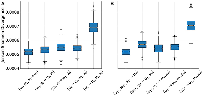
Figure 6. Jensen-Shannon-Divergence (JSD) of true and estimated fields for different cross estimation tasks. In cases where more than one variable is estimated the mean value of the JSDs of the estimated variables is given. (A) Cross estimation for the cases (v_t, w_t, s_t → u_t), (w_t, s_t → u_t, v_t), (u_t, v_t → w_t, s_t), (u_t → v_t, w_t, s_t), and (w_t → u_t, v_t, s_t), based on the input from the BOCF simulation. (B) Cross estimation of future values of not measured variables for the cases $(v_{t^{*}},w_{t^{*}},s_{t^{*}}\to u_{\tau }),(w_{t^{*}},s_{t^{*}}\to u_{\tau },v_{\tau }),(u_{t^{*}},v_{t^{*}}\to w_{\tau },s_{\tau }),(u_{t^{*}}\to v_{\tau },w_{\tau },s_{\tau })$, and $(w_{t^{*}}\to u_{\tau },v_{\tau },s_{\tau })$ based on the forecast of the data driven model for a period of τ = 1, 000, where t* denotes 10 successive snapshots at times 0, 0.1, …, 0.9 constituting the input. In both diagrams the orange line is the median value for each case, the box extends from the lower to upper quartile values. The whiskers extend from the box to show the range of the data. Flier points are those past the end of the whiskers.

4.3. Forecast and Cross-Estimation

This investigation represents a combination of the two previous ones. In this case, however, not for every time step the data from the BOCF model were used, but only ten time steps from the BOCF model were used to initialize the forecast of the network. Depending on the case which variable should be estimated the BOCF variables for initialization were replaced by uniform noise, as before. Figure 6B shows the JSD statistics for the four estimation cases considered and in Figure 7 snapshots of the input and the true and estimated fields are presented illustrating the very good performance at time t = 100.

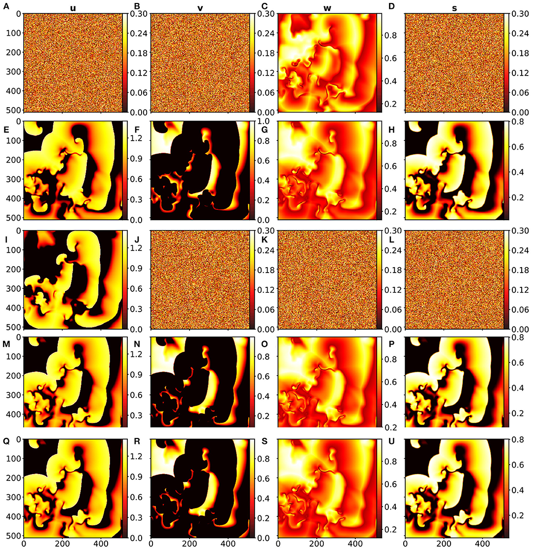
Figure 7. (A–H): Cross estimation of u, v, s at t = 100 based on the input w at t = 0 where (A,B,D) is the random noise input for the system variables u, v and s, (C) is the snapshot input of w at t = 0 (estimation). (E–H) show the output of the data-driven model for the system variables u, v, w, s at time t = 100. (I–P): Cross estimation of v, w, s at t = 100 based on the input u at t = 0 where (I) shows the snapshot input of u at t = 0. (J,K,L) show the random noise input for the system variables v, w and s, (M–P) is the output of the data-driven model for the system variables u, v, w, s at time t = 100 (prediction). (Q–U): Reference data from the BOCF model for time t = 100, where (Q–U) are the snapshots for the system variables u, v, w, and s.

5. Discussion

Spatio-temporal non-linear dynamical systems like extended systems (described by PDEs) or networks of interacting oscillators may exhibit very high dimensional chaotic dynamics. A typical example are complex wave pattern occurring in some excitable media. As a representative of this class of systems we used the BOCF model describing electrical excitation waves in cardiac tissue where chaotic dynamics is associated with cardiac arrhythmias. For future applications like monitoring and predicting the dynamical state of the heart or the impact of interventions, mathematical models are required describing the temporal evolution or the relation between different (physical) variables. As an alternative to the large number of simple qualitative or detailed (ionic) models (incorporating many biophysical details and corresponding variables) we presented a machine learning approach for data driven modeling of the spatio-temporal dynamics. A convolutional neural network combined with a linear-chain of conditional random fields was trained and validated with data generated by a simulation of the BOCF model. To mimic experimental limitations when measuring cardiac dynamics we considered different cases where only some of the variables of the BOCF model were assumed to be available as input of the generated model and the not measurable variables were replace by random numbers. Running the trained network in a closed loop (feedback) configuration iterated prediction provided forecasts of the complex dynamics that turned out to follow the true (chaotic!) evolution of the BOCF simulation for about five periods of the intrinsic spiral rotations. These results clearly show that machine learning methods like those employed here provide faithful models of the underlying complex dynamics of excitable media that, when suitably trained can provide powerful tools for predicting the spatio-temporal evolution and for cross-estimating not directly observed variables.

Author Contributions

SH performed numerical simulations. UP and SH identified the scientific topic. UP, FW, and SH devised the strategy for solving it, and wrote the manuscript.

Funding

SH acknowledges funding by the International Max Planck Research Schools of Physics of Biological and Complex Systems.

Conflict of Interest Statement

The authors declare that the research was conducted in the absence of any commercial or financial relationships that could be construed as a potential conflict of interest.

Acknowledgments

We thank T. Lilienkamp and S. Luther for support with the BOCF model and for inspiring discussions about spatio-temporal dynamics in excitable media.

Supplementary Material

The Supplementary Material for this article can be found online at: https://www.frontiersin.org/articles/10.3389/fams.2018.00060/full#supplementary-material

Supplemental Data. Movie showing the temporal evolution of the u field from the simulation, the forecast and the absolute difference of both.

Footnotes

References

1. Barkley D. A model for fast computer simulation of waves in excitable media. Physica D Nonlinear Phenomena (1991) 49:61–70.
2. Bär M, Eiswirth M. Turbulence due to spiral breakup in a continuous excitable medium. Phys Rev E (1993) 48:R1635–7.
3. Cherry EM, Fenton F, Krogh-Madsen T, Luther S, Parlitz U. Introduction to focus issue: complex cardiac dynamics. Chaos (2017) 27:093701. doi: 10.1063/1.5003940
4. Clayton RH, Bernus O, Cherry EM, Dierckx H, Fenton FH, Mirabella L, et al. Models of cardiac tissue electrophysiology: progress, challenges and open questions. Prog Biophys Mol Biol. (2011) 104:22–48. doi: 10.1016/j.pbiomolbio.2010.05.008
5. Uzelac I, Ji YC, Hornung D, Schrder-Scheteling J, Luther S, Gray RA, et al. Simultaneous quantification of spatially discordant alternans in voltage and intracellular calcium in langendorff-perfused rabbit hearts and inconsistencies with models of cardiac action potentials and Ca transients. Front Physiol. (2017) 8:819. doi: 10.3389/fphys.2017.00819
6. Evensen G, van Leeuwen P. An ensemble Kalman smoother for nonlinear dynamics. Mon Weather Rev. (2000) 128:1852–67. doi: 10.1175/1520-0493(2000)128<1852:AEKSFN>2.0.CO;2
7. Abarbanel HDI. Predicting the Future - Completing Models of Observed Complex Systems. New York, NY: Springer-Verlag (2013).
8. Law K, Stuart A, Zygalakis K. Data Assimilation - A Mathematical Introduction. Cham: Springer International Publishers (2015).
9. Hoffman MJ, LaVigne NS, Scorse ST, Fenton FH, Cherry EM. Reconstructing three-dimensional reentrant cardiac electrical wave dynamics using data assimilation. Chaos (2016) 26:013107. doi: 10.1063/1.4940238
10. Berg S, Luther S, Parlitz U. Synchronization based system identification of an extended excitable system. Chaos (2011) 21:033104. doi: 10.1063/1.3613921
11. Bueno-Orovio A, Cherry EM, Fenton FH. Minimal model for human ventricular action potentials in tissue. J Theor Biol. (2008) 253:544–60. doi: 10.1016/j.jtbi.2008.03.029
12. Box GE, Jenkins GM, Reinsel GC, Ljung GM. Time Series Analysis: Forecasting and Control>. San Francisco, CA: John Wiley & Sons (2015).
13. Solomatine DP, Ostfeld A. Data-driven modelling: some past experiences and new approaches. J Hydroinformatics (2008) 10:3–22. doi: 10.2166/hydro.2008.015
14. Parlitz U, Merkwirth C. Prediction of spatiotemporal time series based on reconstructed local states. Phys Rev Lett. (2000) 84:1890. doi: 10.1103/PhysRevLett.84.1890
15. Jaeger H. The ‘Echo State‘ Approach to Analysing and Training Recurrent Neural Networks - With an Erratum Note. GMD Report (2001).
16. Jäger H, Haas H. Harnessing nonlinearity: predicting chaotic systems and saving energy in wireless communication. Science (2004) 304:78–80. doi: 10.1126/science.1091277
17. Verstraeten D, Schrauwen B, D'Haene M, Stroobandt D. An experimental unification of reservoir computing methods. Neural Netw. (2007) 20:391–403. doi: 10.1016/j.neunet.2007.04.003
18. Pathak J, Hunt B, Girvan M, Lu Z, Ott E. Model-free prediction of large spatiotemporally chaotic systems from data: a reservoir computing approach. Phys Rev Lett. (2018) 120:024102. doi: 10.1103/PhysRevLett.120.024102
19. Zimmermann RS, Parlitz U. Observing spatio-temporal dynamics of excitable media using reservoir computing. Chaos (2018) 28:043118. doi: 10.1063/1.5022276
20. Quade M, Abel M, Nathan Kutz J, Brunton SL. Sparse identification of nonlinear dynamics for rapid model recovery. Chaos (2018) 28:063116. doi: 10.1063/1.5027470
21. Abebe A, Solomatine D, Venneker R. Application of adaptive fuzzy rule-based models for reconstruction of missing precipitation events. Hydrol Sci J. (2000) 45:425–36. doi: 10.1080/02626660009492339
22. Abebe AJ, Guinot V, Solomatine DP. Fuzzy alpha-cut vs. Monte Carlo techniques in assessing uncertainty in model parameters. In: Proc. 4-th International Conference on Hydroinformatics. Iowa City, IA (2000). p. 1–8.
23. Krizhevsky A, Sutskever I, Hinton GE. Imagenet classification with deep convolutional neural networks. In: Advances in Neural Information Processing Systems. Curran Associates Inc. (2012). p. 1097–105.
24. Lafferty JD, McCallum A, Pereira FCN. Conditional Random Fields: Probabilistic Models for Segmenting and Labeling Sequence Data. In: Proceedings of the Eighteenth International Conference on Machine Learning. ICML '01. San Francisco, CA: Morgan Kaufmann Publishers Inc. (2001). p. 282–9.
27. Schmidhuber J. Deep learning in neural networks: an overview. Neural Netw. (2015) 61:85–117. doi: 10.1016/j.neunet.2014.09.003
28. Hinton GE, Salakhutdinov RR. Reducing the dimensionality of data with neural networks. Science (2006) 313:504–7. doi: 10.1126/science.1129198
29. He K, Zhang X, Ren S, Sun J. Deep residual learning for image recognition. arXiv:1512.03385 (2015).
30. Noh H, Hong S, Han B. Learning deconvolution network for semantic segmentation. arXiv:1505.04366 (2015).
31. Chatzis SP, Demiris Y. The infinite-order conditional random field model for sequential data modeling. IEEE Trans Pattern Anal Mach Intell. (2013) 35:1523–34. doi: 10.1109/TPAMI.2012.208
32. Ten Tusscher K, Noble D, Noble P, Panfilov AV. A model for human ventricular tissue. Am J Physiol Heart Circ Physiol. (2004) 286:H1573–89. doi: 10.1152/ajpheart.00794.2003
33. Strain MC, Greenside HS. Size-dependent transition to high-dimensional chaotic dynamics in a two-dimensional excitable medium. Phys Rev Lett. (1998) 80:2306–9. doi: 10.1103/PhysRevLett.80.2306
34. Lilienkamp T, Christoph J, Parlitz U. Features of chaotic transients in excitable media governed by spiral and scroll waves. Phys Rev Lett. (2017) 119:054101. doi: 10.1103/PhysRevLett.119.054101
35. Kingma DP, Ba J. Adam: a method for stochastic optimization. arXiv preprint arXiv:14126980 (2014).
36. Lin J. Divergence measures based on the Shannon entropy. IEEE Trans Inform Theor. (1991) 37:145–51.
38. Gültas M, Düzgün G, Herzog S, Jäger SJ, Meckbach C, Wingender E, et al. Quantum coupled mutation finder: predicting functionally or structurally important sites in proteins using quantum Jensen-Shannon divergence and CUDA programming. BMC Bioinformatics (2014) 15:96. doi: 10.1186/1471-2105-15-96
39. Roberts N. Assessing the spatial and temporal variation in the skill of precipitation forecasts from an NWP model. Meteorol Appl. (2008) 15:163–9. doi: 10.1002/met.57
Keywords: deep learning, conditional random fields, artificial neural network, cross-estimation, spatio-temporal chaos, excitable media, cardiac arrhythmias, non-linear observer
Citation: Herzog S, Wörgötter F and Parlitz U (2018) Data-Driven Modeling and Prediction of Complex Spatio-Temporal Dynamics in Excitable Media. Front. Appl. Math. Stat. 4:60. doi: 10.3389/fams.2018.00060
Received: 04 September 2018; Accepted: 26 November 2018;
Published: 11 December 2018.
Edited by:
Axel Hutt, German Weather Service, GermanyReviewed by:
Christian Andreas Welzbacher, German Weather Service, GermanyXin Tong, National University of Singapore, Singapore
Copyright © 2018 Herzog, Wörgötter and Parlitz. This is an open-access article distributed under the terms of the Creative Commons Attribution License (CC BY). The use, distribution or reproduction in other forums is permitted, provided the original author(s) and the copyright owner(s) are credited and that the original publication in this journal is cited, in accordance with accepted academic practice. No use, distribution or reproduction is permitted which does not comply with these terms.
*Correspondence: Ulrich Parlitz, ulrich.parlitz@ds.mpg.de