Filter Bank Common Spatial Pattern Algorithm on BCI Competition IV Datasets 2a and 2b

The Common Spatial Pattern (CSP) algorithm is an effective and popular method for classifying 2-class motor imagery electroencephalogram (EEG) data, but its effectiveness depends on the subject-specific frequency band. This paper presents the Filter Bank Common Spatial Pattern (FBCSP) algorithm to optimize the subject-specific frequency band for CSP on Datasets 2a and 2b of the Brain-Computer Interface (BCI) Competition IV. Dataset 2a comprised 4 classes of 22 channels EEG data from 9 subjects, and Dataset 2b comprised 2 classes of 3 bipolar channels EEG data from 9 subjects. Multi-class extensions to FBCSP are also presented to handle the 4-class EEG data in Dataset 2a, namely, Divide-and-Conquer (DC), Pair-Wise (PW), and One-Versus-Rest (OVR) approaches. Two feature selection algorithms are also presented to select discriminative CSP features on Dataset 2b, namely, the Mutual Information-based Best Individual Feature (MIBIF) algorithm, and the Mutual Information-based Rough Set Reduction (MIRSR) algorithm. The single-trial classification accuracies were presented using 10 × 10-fold cross-validations on the training data and session-to-session transfer on the evaluation data from both datasets. Disclosure of the test data labels after the BCI Competition IV showed that the FBCSP algorithm performed relatively the best among the other submitted algorithms and yielded a mean kappa value of 0.569 and 0.600 across all subjects in Datasets 2a and 2b respectively.

1. Introduction

The challenge in Motor Imagery-based BCI (MI-BCI), which translates the mental imagination of movement to commands, is the huge inter-subject variability with respect to the characteristics of the brain signals (Blankertz et al., 2007). The Common Spatial Pattern (CSP) algorithm is effective in constructing optimal spatial filters that discriminates 2 classes of electroencephalogram (EEG) measurements in MI-BCI (Blankertz et al., 2008b). For effective use of the CSP algorithm, several parameters have to be specified, namely, the frequency for band-pass filtering of the EEG measurements, the time interval of the EEG measurements taken relative to the stimuli, and the subset of CSP filters to be used (Blankertz et al., 2008b). Typically, general settings such as the frequency band of 7–30 Hz, the time segment starting 1 s after cue, and 2 or 3 subset of CSP filters are used (Blankertz et al., 2008b). However, the performance of the CSP algorithm can be potentially enhanced by subject-specific parameters (Blankertz et al., 2007). Several approaches were proposed to address the issue of selecting optimal temporal frequency band for the CSP algorithm. These include, but not limited to, the Common Spatio-Spectral Pattern (CSSP) which optimizes a simple filter that employed a one time-delayed sample with the CSP algorithm (Lemm et al., 2005); the Common Sparse Spectral-Spatial Pattern (CSSSP) which performs simultaneous optimization of an arbitrary Finite Impulse Response (FIR) filter within the CSP algorithm (Dornhege et al., 2006); and the SPECtrally weighted Common Spatial Pattern (SPEC-CSP) algorithm (Tomioka et al., 2006) which alternately optimizes the temporal filter in the frequency domain and then the spatial filter in an iterative procedure.

In this paper, the Filter Bank Common Spatial Pattern (FBCSP) algorithm is presented to enhance the performance of the CSP algorithm by performing autonomous selection of discriminative subject-specific frequency range for band-pass filtering of the EEG measurements (Ang et al., 2008). The FBCSP algorithm is only effective in discriminating 2 classes of EEG measurements, but the BCI Competition IV Dataset 2a (Tangermann et al., 2012) comprises 4 classes of EEG measurements of motor imagery on the left hand, right hand, foot, and tongue. Therefore, this paper also presents and investigates 3 approaches of multi-class extension to the FBCSP algorithm on Dataset 2a, namely, Divide-and-Conquer (DC), Pair-Wise (PW), and One-Versus-Rest (OVR). In addition, this paper also investigates the performance of the FBCSP algorithm on Dataset 2b (Leeb et al., 2007) using 2 mutual information-based feature selection algorithms.

The remainder of this paper is organized as follows. Section 2 provides a description of the FBCSP algorithm, 3 approaches of multi-class extensions to FBCSP, and 2 mutual information-based feature selection algorithms. Section 3 describes the experimental studies and results on the training data of the BCI Competition IV Datasets 2a and 2b. Finally, section 4 concludes this paper with the results on the evaluation data of both datasets from the competition.

2. Filter Bank Common Spatial Pattern

The Filter Bank Common Spatial Pattern (FBCSP) algorithm (Ang et al., 2008) is illustrated in Figure 1. FBCSP comprises 4 progressive stages of signal processing and machine learning on the EEG data: a filter bank comprising multiple Chebyshev Type II band-pass filters, spatial filtering using the CSP algorithm, CSP feature selection, and classification of selected CSP features. The CSP projection matrix for each filter band, the discriminative CSP features, and the classifier model are computed from training data labeled with the respective motor imagery action. These parameters computed from the training phase are then used to compute the single-trial motor imagery action during the evaluation phase.

FIGURE 1

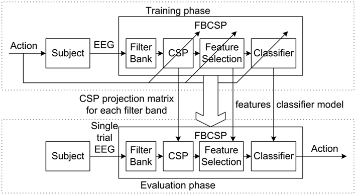
Figure 1. Architecture of the filter bank common spatial pattern (FBCSP) algorithm for the training and evaluation phases.

2.1. Band-Pass Filtering

The first stage employs a filter bank that decomposes the EEG into multiple frequency pass bands using causal Chebyshev Type II filter. A total of 9 band-pass filters are used, namely, 4–8, 8–12, …, 36–40 Hz. Various configurations of the filter bank are as effective, but these band-pass frequency ranges are used because they yield a stable frequency response and cover the range of 4–40 Hz.

2.2. Spatial Filtering

The second stage performs spatial filtering using the CSP algorithm. The CSP algorithm is highly successful in calculating spatial filters for detecting Event-Related Desynchronization/Synchronization (ERD/ERS; Pfurtscheller and Aranibar, 1979; Pfurtscheller and Lopes da Silva, 1999). Each pair of band-pass and spatial filter in the first and second stage performs spatial filtering to EEG measurements that have been band-pass filtered with a specific frequency range. Each pair of band-pass and spatial filter thus computes the CSP features that are specific to the band-pass frequency range. Spatial filtering is performed using the CSP algorithm by linearly transforming the EEG measurements using

where denotes the single-trial EEG measurement from the bth band-pass filter of the ith trial; denotes E _b,i after spatial filtering, denotes the CSP projection matrix; c is the number of channels; t is the number of EEG samples per channel; and T denotes transpose operator.

The CSP algorithm computes the transformation matrix W _b to yield features whose variances are optimal for discriminating 2 classes of EEG measurements (Blankertz et al., 2008a; Ramoser et al., 2000; Müller-Gerking et al., 1999; Fukunaga, 1990) by solving the eigenvalue decomposition problem

where Σ_b,1 and Σ_b,2 are estimates of the covariance matrices of the bth band-pass filtered EEG measurements of the respective motor imagery action, D _b is the diagonal matrix that contains the eigenvalues of Σ_b,1. Technically, W _b can be computed in MATLAB using the command W = eig(S1, S1 + S2) (Blankertz et al., 2008b) where W, S1, and S2 here represents W _b, Σ_b,1, and Σ_b,2 respectively.

The spatial filtered signal Z _b,i in equation (1) using W _b from equation (2) thus maximizes the differences in the variance of the 2 classes of band-pass filtered EEG measurements. The m pairs of CSP features of the ith trial for the bth band-pass filtered EEG measurements are then given by

where represents the first m and the last m columns of W_b; diag(·) returns the diagonal elements of the square matrix; tr[·] returns the sum of the diagonal elements in the square matrix. Note that m = 2 is used for Dataset 2a and m = 1 is used for Dataset 2b.

The FBCSP feature vector for the ith trial is then formed as follows

where i = 1, 2, …, n; n denotes the total number of trials in the data.

The training data that comprised the extracted feature data and the true class labels are denoted as

respectively to make a distinction from the evaluation data, where and denote the feature vector and true class label from the ith training trial, i = 1, 2, …, n_t; and n_t denotes the total number of trials in the training data.

2.3. Feature Selection

The third stage employs a feature selection algorithm to select discriminative CSP features from from equation (5) for the subject’s task. Various feature selection algorithms can be used, but the Mutual Information-based Best Individual Feature (MIBIF) and the Mutual Information-based Rough Set Reduction (MIRSR) algorithm are employed during the competition. During cross-validation, the input data is split randomly into training data and validation data. These 2 algorithms performs feature selection only on the training data by selecting the discriminative CSP features based on the mutual information computed between each feature and the corresponding motor imagery classes. These 2 algorithms are described in the following subsections.

2.3.1. Mutual information-based best individual feature algorithm

The Mutual Information-based Best Individual Feature (MIBIF) algorithm (Ang and Quek, 2006; Jain et al., 2000) is based on the filter approach. The mutual information of each feature is computed and sorted in descending order. The first k features are then selected. The MIBIF algorithm is described as follows:

• Step 1: Initialization. Initialize set of features from equation (5) and set of true labels from equation (6) whereby is the jth column vector of , and the true label of each trial

Initialize set of selected features = ∅.

• Step 2: Compute the mutual information of each feature f _j∈ with each class label ω = {1, 2} ∈

Compute I (f _j; ω)∀j = 1, 2, …(9 _* 2m) using

where and the conditional entropy is

where is the feature value of the ith trial from f_j.

The probability p(ω | f_j,i) can be computed using Bayes rule given in equations (9) and (10).

where p(ω | f_j,i) is the conditional probability of class ω given f_j,i; p(f_j,i | ω) is the conditional probability of f_j,i given class ω; P(ω) is the prior probability of class ω; and p(f_j,i) is

The conditional probability p(f_j,i | ω) can be estimated using Parzen Window (Parzen, 1962) given by

where n_ω is the number of data samples belonging to class ω; I_ω is the set of indices of the training data trials belonging to class ω; f_j,k is the feature value of the kth trial from f _j and Φ is a smoothing kernel function with a smoothing parameter h given in equations (20) and (21) respectively.

• Step 3: Sort all the features in descending order of mutual information computed in step 2 and select the first k features. Mathematically, this step is performed as follows till |S| = k

where \ denotes set theoretic difference; ∪ denotes set union; and | denotes given the condition.

Based on the study in (Ang et al., 2008), k = 4 is used. Note that since the CSP features are paired, the corresponding pair of features is also included if it is not selected. After performing feature selection on the feature selected training data is denoted as where d ranges from 4 to 8. d = 4 if all 4 features selected are from 2 pairs of CSP features. d = 8 if all 4 features selected are from 4 pairs of CSP features, since their corresponding pair is included.

2.3.2. Mutual information-based rough set theory algorithm

The Mutual Information-based Rough Set Reduction (MIRSR) algorithm is based on the wrapper approach for the Rough set-based Neuro-Fuzzy System (RNFS). It employs the mutual information to select attributes with high relevance and the concept of knowledge reduction in rough set theory to select attributes with low redundancy (Ang and Quek, 2006). The MIRSR algorithm is described as follows:

• Step 1: Generation of fuzzy membership functions. Initialize set of features from equation (5) and set of true labels from equation (6) whereby is the jth column vector of and the true label of each trial Generate fuzzy membership functions of feature f _j using the Supervised Pseudo Self-Evolving Cerebellar (SPSEC) algorithm (Ang and Quek, 2012) for j = 1, 2,…, (9 _* 2m).

• Step 2: Compute the mutual information of each feature f _j∈ with each class label ω = {1, 2} ∈ Given f _j= [x_1,j,…x_i,j,…x_n,j] for n trials in the training data, perform classification of each x_i,j using the membership functions generated.

Estimate p(ω | f _j) from the number of correct classifications for class ω using the membership functions generated.

Compute I (f _j; ω)∀j = 1, 2,…(9 * 2m) using

where

and the conditional entropy is

• Step 3: Select best k features. Sort all the features in descending order of mutual information computed in step 2 and select the first k = 2log₂ (9 * 2m) features.

• Step 4: Remove redundant features. Remove membership functions that are not selected from step 3 and perform reduction using step 2 of the Rough Set Pseudo Outer-Product (RSPOP) algorithm (Ang and Quek, 2005). Similar to the MIBIF algorithm, after performing feature selection on the feature selected training data is denoted as and the corresponding pairs of CSP features are selected.

2.4. Classification

The 4th stage employs a classification algorithm to model and classify the selected CSP features. Various classification algorithms can be used, but the study in (Ang et al., 2008) showed that FBCSP that employed the Naïve Bayesian Parzen Window (NBPW) classifier (Ang and Quek, 2006) yielded better results on the BCI Competition III Dataset IVa. Therefore, the following NBPW algorithm is used.

Given that denotes the entire training data of n trials, denotes the training data with the d selected features from the ith trial, and x = [x₁, x₂, …x_d] denotes a random evaluation trial; the NBPW classifier estimates p(x | ω) and P(ω) from training data samples and predicts the class ω with the highest posterior probability p(ω | x) using Bayes rule

where p(ω | x) is the conditional probability of class ω given random trial x; p(x | ω) is the conditional probability of x given class ω; P(ω) is the prior probability of class ω; and p(x) is

The computation of p(ω | x) is rendered feasible by a naïve assumption that all the features x₁, x₂,…, x_d are conditionally independent given class ω in

The NBPW classifier employs Parzen Window (Parzen, 1962) to estimate the conditional probability p(x_j | ω) in

where n_ω is the number of data samples belonging to class ω; I_ω is the set of indices of the training data trials belonging to class ω; and Φ is a smoothing kernel function with a smoothing parameter h. The NBPW classifier employs the univariate Gaussian kernel given by

and normal optimal smoothing strategy (Bowman and Azzalini, 1997) given by

where σ denotes the standard deviation of the distribution of y.

The classification rule of the NBPW classifier is given by

The CSP algorithm was proposed for the binary classification of single-trial EEG (Ramoser et al., 2000), and several multi-class extensions of the CSP algorithm have been proposed (Dornhege et al., 2004a; Dornhege et al., 2004b; Grosse-Wentrup and Buss, 2008). Some examples of multi-class extensions include: using CSP within the classifier, One-Versus-Rest (OVR) and simultaneous diagonalization of covariance matrices from the multi-class data. This section describes the 3 proposed approaches of multi-class extensions to the FBCSP algorithm to address the BCI Competition IV Dataset 2a, namely, Divide-and-Conquer (DC), Pair-Wise (PW), and One-Versus-Rest (OVR).

2.5. Divide-and-Conquer

Given that ω, ω′ ∈ {1, 2, 3, 4} represents the left, right, foot, and tongue motor imagery, the Divide-and-Conquer (DC) approach adopts a tree-based classifier approach (Zhang et al., 2007; Chin et al., 2009). For the 4 classes of motor imagery in the BCI Competition IV Dataset 2a, 4 − 1 = 3 binary classifiers are required. The classification rule of the NBPW classifier is thus extended from equation (22) to

where p_DC(ω | x) is the probability of classifying a random trial x between class ω and class ω′; and p(ω′ | x) = 0 if ω′ = Ø.

For example, for the DC classifier where ω = 1, ω′ = {2, 3, 4}. Hence, class 1 is first discriminated from classes 2, 3, and 4. If the random trial sample is classified as class ω, the classification procedure stops. If the random trial sample is classified as class ω′, then the decision is deferred to the next DC classifier where ω = 2, ω′ = {3, 4}. Finally, if the random trial sample is classified as class ω′, then the decision is deferred to the last DC classifier where ω = 3, ω′ = 4.

2.6. Pair-Wise

Given that ω, ω′ ∈ {1, 2, 3, 4} represents the left, right, foot, and tongue motor imagery, the Pair-Wise (PW) approach computes the CSP features that discriminates every pair of classes (Müller-Gerking et al., 1999; Duda et al., 2001). For the 4 classes of motor imagery in the BCI Competition IV Dataset 2a, 4 _* (4 − 1)/2 = 6 binary classifiers are required to discriminate between class ω and ω′. The classification rule of the NBPW classifier is thus extended from equation (22) to a majority voting scheme based on the predicted class labels from the binary classifiers using

where p_PW(ω | x) is the probability of classifying a random trial x between class ω and class ω′; and the absolute operator |·| here returns 1 if it is true and 0 otherwise. In case of a draw in the majority voting scheme, the class label with a smaller ω is chosen.

For example, for the PW classifier where ω = 2, ω′ = 1, 3, or 4; class 2 is discriminated from classes 1, 3, and 4 using 3 PW classifiers.

2.7. One-Versus-Rest

Given that ω, ω′ ∈ {1, 2, 3, 4} represents the left, right, foot, and tongue motor imagery, the OVR approach computes the CSP features that discriminates each class from the rest of the classes (Dornhege et al., 2004b; Duda et al., 2001). For the 4 classes of motor imagery in the BCI Competition IV Dataset 2a, 4 binary classifiers are required. The classification rule of the NBPW classifier is thus extended from equation (22) to

where p_OVR(ω | x) is the probability of classifying a random trial x between class ω and class ω′ = {1, 2, 3, 4}ω; and \ denotes the set theoretic difference operation.

For example, in the OVR classifier where , ω′ = {1, 3, 4}; class 2 is discriminated from the aggregated classes 1, 3, and 4.

3. Experimental Results

The performances of the algorithms were evaluated on BCI Competition IV (Tangermann et al., 2012) Dataset 2a and Dataset 2b. During the competition, only the class labels for the training data were provided while the class labels for the evaluation data were disclosed only after the competition results have been announced. Furthermore, the competition rules stipulated that the algorithms for both datasets should be causal and the predicted labels for each time sample from the onset of the fixation cross to the end of motor imagery should also be submitted. The performances were judged based on the maximum Kappa value achieved on the evaluation data.

3.1. Dataset 2a

BCI Competition IV (Tangermann et al., 2012) Dataset 2a comprised 4 classes of motor imagery EEG measurements from 9 subjects, namely, left hand, right hand, feet, and tongue. Two sessions, one for training and the other for evaluation, were recorded from each subject. Each session comprised 288 trials of data recorded with 22 EEG channels and 3 monopolar electrooculogram (EOG) channels (with left mastoid serving as reference). The performance of the FBCSP algorithm on the 4-class motor imagery data was evaluated by employing the 3 approaches of multi-class extension (DC, PW, and OVR) to FBCSP using the MIBIF feature selection algorithm.

3.1.1. Protocol

Figure 2 illustrates how the single-trial EEG data were extracted for training the FBCSP algorithm on Dataset 2a. The setting of m = 2 pairs of CSP features for the band-pass filtered EEG measurements, and the time segment of 0.5–2.5 s after the onset of the visual cue were used. Figure 2 also shows that the FBCSP algorithm performed the computation using a 2-s window of EEG data at any point in time, and the classification output of a time sample was computed from the previous 2 s of EEG data to satisfy the causality criterion. To compute the classification output of a single-trial, the EEG data labeled as test_time_segment starting from −2 s from the onset of the fixation cross to the end of motor imagery was used. In addition, to account for the transitional effects of the causal filters, an additional 0.5 s of EEG data was extracted on both ends of test_time_segment, labeled as extract_time_segment. As the computation of every time point of the evaluation data was computationally intensive, the classification output was only computed on every alternate 10th time sample, and a zero-order hold was used to map back to every time sample.

FIGURE 2

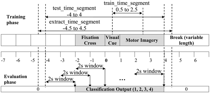
Figure 2. The illustration on the extraction of a single-trial EEG segment from the training data for the multi-class FBCSP training phase in Dataset 2a, and the generation of the classification outputs using the multi-class extension to FBCSP on the entire time segment of a single-trial for the evaluation phase.

3.1.2. Cross-validation results

The single-trial classification performances of the 3 approaches of multi-class extensions to the FBCSP algorithm were first investigated on the training data. The performance was evaluated in terms of the mean kappa value using 10 × 10-fold cross-validations. The results on the training data from Dataset 2a are shown in Table 1.

TABLE 1

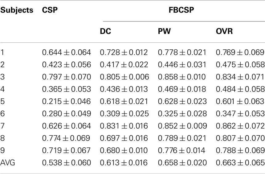
Table 1. 10 × 10-fold cross-validation performance in terms of maximum kappa value using CSP and the 3 approaches of multi-class extensions to FBCSP on the training data from BCI Competition IV Dataset 2a.

The results showed that the OVR extension to FBCSP yielded the best averaged mean kappa value (0.663). A paired t-test revealed no significant difference between the OVR and PW approaches (p = 0.480), and a significant difference between the OVR and DC approaches (p = 0.006). The DC approach yielded the worst performance among the 3 approaches of multi-class extensions to FBCSP. This may be due to the fact that the DC approach performed classification on 4 classes of motor imagery by employing only 3 classifiers, which is relatively lesser than the PW and OVR approaches. Furthermore, the classification order in the DC approach could be optimized to yield improved performance. Since there existed 12 possible permutations of the DC classification order, an exhaustive search on the optimal classification order for each subject based on 10 × 10-fold cross-validation results would have been computationally expensive and hence this was not performed. Instead, the order of classification for each subject was determined by ranking each class based on the cross-validation results of classifying against the other classes. The OVR approach yielded the best averaged mean kappa value, and it performed the best in 6 subjects (2, 4, 6, 7, 8, and 9) while the PW approach performed the best in 3 subjects (1, 3, and 5). Furthermore, the OVR approach was less computationally expensive compared to the PW approach as it used 4 classifiers whereas the PW approach used 6 classifiers. Based on these observations, the OVR approach of multi-class extension to the FBCSP algorithm was selected for the submission to the competition.

For comparative purposes, Table 1 also included the results on the OVR approach of multi-class extension to the CSP algorithm that employed a 7–35 Hz band-pass filter. The results showed that the FBCSP algorithm consistently outperforms the CSP algorithm for all 9 subjects, and a paired t-test revealed significant difference between these 2 algorithms (p = 0.012) employing the OVR multi-class extension.

3.1.3. Unseen evaluation data results

The results of the FBCSP algorithm on the evaluation data for BCI Competition IV Dataset 2a are shown in Table 2.

TABLE 2

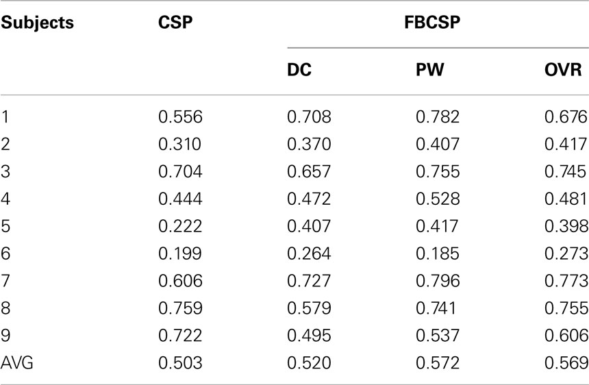
Table 2. Classification results from using CSP and the 3 approaches of multi-class extensions to FBCSP algorithm on the unseen evaluation data from BCI Competition IV Dataset 2a.

The results showed that the PW extension to FBCSP yielded the best averaged mean kappa value (0.572). A paired t-test revealed no significant difference between the OVR and PW approaches (p = 0.898), and no significant difference between the OVR and DC approaches (p = 0.055). The DC approach yielded relatively the worst performance among the 3 approaches. The PW approach yielded slightly higher mean kappa value compared to OVR and it performed the best in 5 subjects (1, 3, 4, 5, 7) whereas the OVR approach performed the best in 4 subjects (2, 6, 8, 9). Both the OVR and PW approach yielded a mean kappa value of approximately 0.57 across the 9 subjects, which would achieve the best performance relative to all the other entries submitted to the competition.

For comparative purposes, Table 2 also included the results of the OVR approach of multi-class extension on the CSP algorithm that employed a 7–35 Hz band-pass filter. A paired t-test revealed no significant difference between the FBCSP algorithm and the CSP algorithm employing the OVR approach of multi-class extensions (p = 0.059). Nevertheless, the results showed that the FBCSP algorithm yielded a better mean kappa value and it outperformed the CSP algorithm in 8 of the 9 subjects (except subject 8).

Comparing the results of Tables 1 and 2, the results on the evaluation data were consistently lower than the cross-validation results for all 3 approaches. Specifically, the OVR approach of multi-class extension to the FBCSP algorithm yielded lower mean kappa value averaged over all the subjects on the evaluation data (0.569) than the cross-validation results (0.663) in all the 9 subjects.

3.2. Dataset 2b

BCI Competition IV (Tangermann et al., 2012) Dataset 2b comprised 2 classes of motor imagery EEG measurements from 9 subjects, namely, left and right hand based on the experiment protocol in (Leeb et al., 2007). Five sessions were recorded from each subject. Each session comprised EEG data recorded from 3 bipolar recordings (C3, Cz, and C4) and 3 monopolar EOG channels. The training data, which consisted the first 2 sessions and the 3rd session, comprised 240 trials without visual feedback and 160 trials with visual feedback respectively. The evaluation data consisted 2 sessions of EEG data that comprised a total of 320 trials. The performance of the FBCSP algorithm on the 2-class motor imagery data was evaluated by employing FBCSP using the MIBIF and MIRSR feature selection algorithms.

3.2.1. Protocol

Figure 3 illustrates how the single-trial EEG data were extracted for training the FBCSP algorithm on Dataset 2b. The protocol used was similar to the protocol for Dataset 2a whereby the time segment of 0.5–2.5 s after the onset of the visual cue was used to train the FBCSP algorithm. However, the setting of m in Dataset 2b was constrained by the 3 EEG channels available for spatial filtering. Hence, the setting of m = 1 pair of CSP features was used.

FIGURE 3

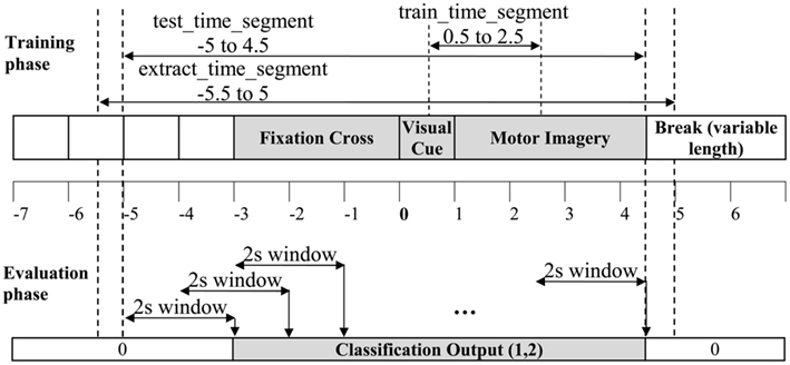
Figure 3. The illustration on the extraction of a single-trial EEG segment from the training data for the FBCSP training phase in Dataset 2b, and the generation of the classification outputs using FBCSP on the entire time segment of a single-trial for the evaluation phase.

3.2.2. Cross-validation results

The single-trial classification performances of the FBCSP algorithm using the 2 feature selection algorithms were first investigated on the training data. The performance was evaluated in terms of the mean kappa value using 10 × 10-fold cross-validations and the results of using all the training sessions from Dataset 2b are shown in Table 3.

TABLE 3

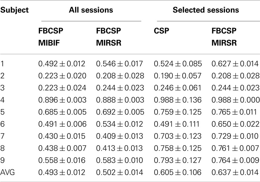
Table 3. 10 × 10-fold cross-validation performance in terms of maximum kappa value using the FBCSP algorithm employing the MIBIF and MIRSR feature selection algorithms on all the sessions of the training data, and using CSP and the FBCSP algorithm employing the MIRSR feature selection algorithm on selected sessions of the training data from BCI Competition IV Dataset 2b.

The results on using all the training sessions showed that the MIRSR feature selection algorithm yielded better averaged mean kappa value (0.502) compared to the use of the MIBIF feature selection algorithm. A paired t-test on the results revealed no significant difference between the MIRSR and MIBIF feature selection algorithms (p = 0.369). The results also showed that the MIRSR feature selection algorithm also performed the best in 5 subjects (1, 3, 5, 6, and 9) whereas the use of the MIBIF algorithm performed the best in 4 subjects (2, 4, 7, and 8). Based on these observations, the MIRSR feature selection algorithm was selected for submission to the competition.

Subsequently, an exhaustive search using 10 × 10-fold cross-validation was carried out to investigate whether the inclusion or exclusion of the first 2 training data sessions would impact the performance of the FBCSP algorithm employing the MIRSR feature selection algorithm. This was because the first 2 training sessions did not involve visual feedback, whereas the 3rd training session involved visual feedback. Based on the exhaustive search, only the 3rd training session was employed to train the FBCSP algorithm for 6 subjects (4, 5, 6, 7, 8, and 9). For subject 1, only the 1st and 3rd training session was employed. For subject 2 and 3, all 3 training sessions were used. The cross-validation results for using the selected sessions are also presented in Table 3. The selected sessions yielded a higher mean kappa value (0.637) compared to using all the sessions (0.502) and the paired t-test revealed a significant difference between the results obtained using the selected sessions and using all sessions (p = 0.012).

For comparative purposes, Table 3 also included the results of the CSP algorithm employing a 7–35 Hz band-pass filter on the selected sessions. Although the paired t-test revealed no significant difference between the FBCSP algorithm and the CSP algorithm (p = 0.151), the results showed that the FBCSP algorithm yielded a better mean kappa value and it outperformed the CSP algorithm in 6 of the 9 subjects (except subjects 3, 4, and 9).

3.2.3. Unseen evaluation data results

The results of the FBCSP algorithm using the selected training sessions on the evaluation data for BCI Competition IV Dataset 2b are shown in Table 4.

TABLE 4

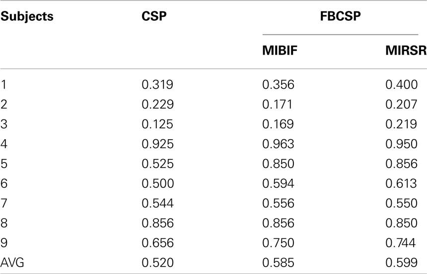
Table 4. Classification results from using CSP and the FBCSP algorithm on the unseen evaluation data from BCI Competition IV Dataset 2b.

The results showed that the FBCSP using the MIRSR feature selection algorithm yielded a better averaged mean kappa value (0.599). The paired t-test revealed no significant difference between the two feature selection algorithms (p = 0.127). The results also showed that the FBCSP using the MIRSR feature selection algorithm performed the best in 5 subjects (1, 2, 3, 5, and 6) whereas the use of the MIBIF algorithm performed the best in 4 subjects (4, 7, 8, and 9). Regardless of the choice, the FBCSP algorithm that employed either the MIBIF or MIRSR feature selection algorithm would yield relatively the best performance in terms of mean kappa value among the other submissions to the competition.

For comparative purposes, Table 4 also included results of using the CSP algorithm that employed a 7–35 Hz band-pass filter. The paired t-test revealed no significant difference between the FBCSP algorithm and the CSP algorithm (p = 0.057). The results showed that the FBCSP algorithm that employed the MIRSR feature selection algorithm also yielded a higher mean kappa value (0.599) and it outperformed the CSP algorithm in 7 out of the 9 subjects (except subjects 2 and 8).

Comparing the results of Tables 3 and 4, the FBCSP algorithm that employed MIRSR yielded lower mean kappa value averaged over all the subjects on the evaluation data (0.599) than on the cross-validation results (0.637), in 7 out of the 9 subjects (except subjects 5 and 8).

4. Conclusion

In this paper, the FBCSP algorithm is presented to classify single-trial EEG data for 2-class as well as 4-class motor imagery, where results using different feature selection algorithms and multi-class extensions to the FBCSP algorithm were compared with the CSP algorithm and other entries submitted to the BCI Competition IV Dataset 2a and Dataset 2b. Although other algorithms were not included in this study, prior studies on the 2-class motor imagery data of the BCI Competition III Dataset IV showed that a modified SPEC-CSP algorithm using Support Vector Machines (SVM) yielded a 10 × 10-fold cross-validation classification accuracy of 89.5% (Wu et al., 2008) averaged over the 5 subjects, while the FBCSP algorithm yielded a 10 × 10-fold cross-validation classification accuracy of 90.3% (Ang et al., 2008). Although they might not be directly comparable, results from these prior studies suggest that the SPEC-CSP algorithm might yield similar results as the FBCSP algorithm in Dataset 2a and 2b as well.

The results on the Filter Bank Common Spatial Pattern (FBCSP) algorithm showed that it is capable of performing an autonomous selection of discriminative subject-specific frequency range for band-pass filtering of the EEG measurements. In the 2-class motor imagery data in Dataset 2b, even though the EEG data was limited to 3 bipolar recordings, the FBCSP algorithm yielded the best performance among all the submissions by employing either the Mutual Information-based Rough Set Reduction (MIRSR) or Mutual Information-based Best Individual Features (MIBIF) feature selection algorithm. The MIBIF feature selection algorithm is dependent on a meta parameter, the number of features selected, which was set-based on the results obtained on the 2-class motor imagery data from the previous BCI Competition III Dataset 4a in Ang et al. (2008). Hence further improvement using the MIBIF feature selection algorithm might be possible by optimizing the number of selected features via a nested cross-validation approach instead. In the 4-class motor imagery data in Dataset 2a, even though the FBCSP algorithm was initially designed for 2-class motor imagery, the results on the 4-class motor imagery data in Dataset 2a showed that the one-versus-the-rest (OVR) and the pair-wise (PW) approaches of multi-class extension to the FBCSP algorithm could also yield relatively the best performance as well.

Conflict of Interest Statement

The authors declare that the research was conducted in the absence of any commercial or financial relationships that could be construed as a potential conflict of interest.

Acknowledgments

The authors would like to thank the organizers and the dataset providers of the BCI Competition IV Dataset 2a and 2b (Tangermann et al., 2012).

References

Ang, K. K., Chin, Z. Y., Zhang, H., and Guan, C. (2008). “Filter bank common spatial pattern (FBCSP) in brain-computer interface,” in Proceedings of the IEEE International Joint Conference on Neural Networks, Hong Kong, 2391–2398.

Ang, K. K., and Quek, C. (2005). RSPOP: rough set-based pseudo outer-product fuzzy rule identification algorithm. Neural Comput. 17, 205–243.

Pubmed Abstract | Pubmed Full Text | CrossRef Full Text

Ang, K. K., and Quek, C. (2006). “Rough set-based neuro-fuzzy system,” in Proceedings of the IEEE International Joint Conference on Neural Networks, Vancouver, BC, 742–749.

Ang, K. K., and Quek, C. (2012). Supervised pseudo self-evolving cerebellar algorithm for generating fuzzy membership functions. Expert Syst. Appl. 39, 2279–2287.

CrossRef Full Text

Blankertz, B., Dornhege, G., Krauledat, M., Müller, K.-R., and Curio, G. (2007). The non-invasive Berlin brain-computer interface: fast acquisition of effective performance in untrained subjects. Neuroimage 37, 539–550.

Pubmed Abstract | Pubmed Full Text | CrossRef Full Text

Blankertz, B., Losch, F., Krauledat, M., Dornhege, G., Curio, G., and Müller, K. R. (2008a). The Berlin brain–computer interface: accurate performance from first-session in BCI-naive subjects. IEEE Trans. Biomed. Eng. 55, 2452–2462.

CrossRef Full Text

Blankertz, B., Tomioka, R., Lemm, S., Kawanabe, M., and Müller, K.-R. (2008b). Optimizing spatial filters for robust EEG single-trial analysis. IEEE Signal Process. Mag. 25, 41–56.

CrossRef Full Text

Bowman, A. W., and Azzalini, A. (1997). Applied Smoothing Techniques for Data Analysis: The Kernel Approach with S-Plus Illustrations. New York: Oxford University Press.

Chin, Z. Y., Ang, K. K., Wang, C., Guan, C., and Zhang, H. (2009). “Multi-class filter bank common spatial pattern for four-class motor imagery BCI,” in Proceedings of the 31st Annual International Conference of the IEEE Engineering in Medicine and Biology Society, Minneapolis, 571–574.

Dornhege, G., Blankertz, B., Curio, G., and Müller, K.-R. (2004a). Boosting bit rates in noninvasive EEG single-trial classifications by feature combination and multiclass paradigms. IEEE Trans. Biomed. Eng. 51, 993–1002.

CrossRef Full Text

Dornhege, G., Blankertz, B., Curio, G., and Müller, K.-R. (2004b). Increase Information Transfer Rates in BCI by CSP Extension to Multi-Class, Vol. 16. Cambridge, MA: MIT Press.

Dornhege, G., Blankertz, B., Krauledat, M., Losch, F., Curio, G., and Müller, K.-R. (2006). Combined optimization of spatial and temporal filters for improving brain-computer interfacing. IEEE Trans. Biomed. Eng. 53, 2274–2281.

Pubmed Abstract | Pubmed Full Text | CrossRef Full Text

Duda, R. O., Hart, P. E., and Stork, D. G. (2001). Pattern Classification, 2nd Edn. New York: John Wiley.

Fukunaga, K. (1990). Introduction to Statistical Pattern Recognition, 2nd Edn. New York: Academic Press.

Grosse-Wentrup, M., and Buss, M. (2008). Multiclass common spatial patterns and information theoretic feature extraction. IEEE Trans. Biomed. Eng. 55, 1991–2000.

Pubmed Abstract | Pubmed Full Text | CrossRef Full Text

Jain, A. K., Duin, R. P. W., and Jianchang, M. (2000). Statistical pattern recognition: a review. IEEE Trans. Pattern Anal. Mach. Intell. 22, 4–37.

CrossRef Full Text

Leeb, R., Lee, F., Keinrath, C., Scherer, R., Bischof, H., and Pfurtscheller, G. (2007). Brain-computer communication: motivation, aim, and impact of exploring a virtual apartment. IEEE Trans. Neural Syst. Rehabil. Eng. 15, 473–482.

Pubmed Abstract | Pubmed Full Text | CrossRef Full Text

Lemm, S., Blankertz, B., Curio, G., and Müller, K.-R. (2005). Spatio-spectral filters for improving the classification of single trial EEG. IEEE Trans. Biomed. Eng. 52, 1541–1548.

Pubmed Abstract | Pubmed Full Text | CrossRef Full Text

Müller-Gerking, J., Pfurtscheller, G., and Flyvbjerg, H. (1999). Designing optimal spatial filters for single-trial EEG classification in a movement task. Clin. Neurophysiol. 110, 787–798.

Pubmed Abstract | Pubmed Full Text | CrossRef Full Text

Parzen, E. (1962). On estimation of a probability density function and mode. Ann. Math. Stat. 33, 1065–1076.

CrossRef Full Text

Pfurtscheller, G., and Aranibar, A. (1979). Evaluation of event-related desynchronization (ERD) preceding and following voluntary self-paced movement. Electroencephalogr. Clin. Neurophysiol. 46, 138–146.

Pubmed Abstract | Pubmed Full Text | CrossRef Full Text

Pfurtscheller, G., and Lopes da Silva, F. H. (1999). Event-related EEG/MEG synchronization and desynchronization: basic principles. Clin. Neurophysiol. 110, 1842–1857.

Pubmed Abstract | Pubmed Full Text | CrossRef Full Text

Ramoser, H., Müller-Gerking, J., and Pfurtscheller, G. (2000). Optimal spatial filtering of single trial EEG during imagined hand movement. IEEE Trans. Rehabil. Eng. 8, 441–446.

Pubmed Abstract | Pubmed Full Text | CrossRef Full Text

Tangermann, M., Müller, K.-R., Aertsen, A., Birbaumer, N., Braun, C., Brunner, C., Leeb, R., Mehring, C., Miller, K. J., Müller-Putz, G., Nolte, G., Pfurtscheller, G., Preissl, H., Schalk, G., Schlögl, A., Vidaurre, C., Waldert, S., and Blankertz, B. (2012). Review of the BCI competition IV. Front. Neurosci. (in press).

Tomioka, R., Dornhege, G., Nolte, G., Blankertz, B., Aihara, K., and Müller, K.-R. (2006). Spectrally Weighted Common Spatial Pattern Algorithm for Single Trial EEG Classification. Mathematical Engineering Technical Reports, University of Tokyo, Tokyo.

Wu, W., Gao, X., Hong, B., and Gao, S. (2008). Classifying single-trial EEG during motor imagery by iterative spatio-spectral patterns learning (ISSPL). IEEE Trans. Biomed. Eng. 55, 1733–1743.

Pubmed Abstract | Pubmed Full Text | CrossRef Full Text

Zhang, D., Wang, Y., Gao, X., Hong, B., and Gao, S. (2007). An algorithm for idle-state detection in motor-imagery-based brain-computer interface. Comput. Intell. Neurosci. 2007, 5.