The pipeline system for Octave and Matlab (PSOM): a lightweight scripting framework and execution engine for scientific workflows
- 1Centre de Recherche de l'Institut Universitaire de Gériatrie de Montréal, Montréal, QC, Canada
- 2Département d'Informatique et de Recherche Opérationnelle, Université de Montréal, Montréal, QC, Canada
- 3McConnell Brain Imaging Centre, Montreal Neurological Institute, McGill University, Montréal, QC, Canada
- 4Mouse Imaging Centre, The Hospital for Sick Children, Toronto, ON, Canada
- 5Department of Medical Biophysics, University of Toronto, Toronto, ON, Canada
- 6Biospective Incorporated, Montréal, QC, Canada
The analysis of neuroimaging databases typically involves a large number of inter-connected steps called a pipeline. The pipeline system for Octave and Matlab (PSOM) is a flexible framework for the implementation of pipelines in the form of Octave or Matlab scripts. PSOM does not introduce new language constructs to specify the steps and structure of the workflow. All steps of analysis are instead described by a regular Matlab data structure, documenting their associated command and options, as well as their input, output, and cleaned-up files. The PSOM execution engine provides a number of automated services: (1) it executes jobs in parallel on a local computing facility as long as the dependencies between jobs allow for it and sufficient resources are available; (2) it generates a comprehensive record of the pipeline stages and the history of execution, which is detailed enough to fully reproduce the analysis; (3) if an analysis is started multiple times, it executes only the parts of the pipeline that need to be reprocessed. PSOM is distributed under an open-source MIT license and can be used without restriction for academic or commercial projects. The package has no external dependencies besides Matlab or Octave, is straightforward to install and supports of variety of operating systems (Linux, Windows, Mac). We ran several benchmark experiments on a public database including 200 subjects, using a pipeline for the preprocessing of functional magnetic resonance images (fMRI). The benchmark results showed that PSOM is a powerful solution for the analysis of large databases using local or distributed computing resources.
1. Introduction
The rapid development of public databases in neuroimaging (e.g., Evans, 2006; Biswal et al., 2010; Burton, 2011) is opening exciting avenues for data mining. The analysis of a neuroimaging database typically involves a large number of inter-connected processing steps, collectively referred to as a pipeline (or workflow) (Deelman et al., 2009). Neuroimaging pipelines can be implemented as a Matlab script, e.g., DPARSF (Chao-Gan and Yu-Feng, 2010), fMRIstat1 (Worsley et al., 2002), SPM2 (Ashburner, 2011), or brainstorm3 (Tadel et al., 2011). Matlab is a programming language for general scientific computing, well-adapted to the rapid prototyping of new algorithms. It can also wrap heterogeneous tools implemented in a variety of languages. To facilitate the inclusion of these computational tools in complex scientific workflows, we developed a general-purpose pipeline system in Octave and Matlab (PSOM)4. To contrast PSOM against alternative projects, we reviewed key features of popular packages within four areas of a pipeline life cycle (Deelman et al., 2009): (1) composition of the pipeline; (2) mapping of the pipeline to the underlying resources; (3) execution of the pipeline; (4) recording of the metadata and provenance.
1.1. Pipeline Composition
The composition of a pipeline is the generation of a (possibly abstract) representation of all steps of analysis and associated dependencies, including access to datasets. Many extensions of existing languages have been developed for that purpose, such as matlabbatch5 for Matlab, or Nipype6 (Gorgolewski et al., 2011) and the Soma-workflow7 (Laguitton et al., 2011) for Python. Some scripting languages were also developed specifically to compose pipelines, e.g., DAGMan8, Swift9 (Wilde et al., 2011) and Pegasus (Deelman et al., 2005). All these systems differ by the way the dependencies between jobs are encoded. DAGMan and Soma-workflow are both based on an explicit declaration of dependencies between jobs by users. The pipeline thus takes the form of a directed acyclic graph (DAG) with jobs as nodes and dependencies as (directed) edges. The Pegasus package also uses a DAG as input, yet this DAG is represented in an XML format called DAX. DAX graphs can be generated by any scripting language. By contrast, Nipype, Swift, and PSOM build on the notion of futures (Baker and Hewitt, 1977), i.e., a list of datasets (or variables) that will be generated by a job at run-time. The data-flow then implicitly defines the dependencies: all the inputs of a job have to exist before it can be started. An alternative to scripting approaches for pipeline composition is to rely on graphical abstractions. A number of projects offer sophisticated interfaces based on “box and arrow” graph representations, e.g., Kepler10 (Ludäscher et al., 2006), Triana11 (Harrison et al., 2008), Taverna12 (Oinn et al., 2006), VisTrails13 (Callahan et al., 2006), Galaxy (Goecks et al., 2010) and LONI pipeline14 (Dinov et al., 2009). Because the graph representations can get really large, various mechanisms have been developed to keep the representation compact, such as encapsulation (the ability to represent a sub-pipeline as one box) and the use of control operations, e.g., iteration of a module over a grid of parameters, instead of a pure data-flow dependency system. Note that complex control mechanism are also necessary in systems geared toward data-flow dependencies to give the ability to, e.g., branch between pipelines or iterate a subpart of the pipeline until a data-dependent condition is satisfied. Finally, systems that put a strong emphasis on pipeline composition and re-use, such as Taverna, Nipype, and LONI pipeline, critically depend on the availability of a library of modules to build pipelines. Taverna claims to have over 3500 such modules, developed in a variety of domains such as bioinformatics or astronomy. Nipype and LONI both offer extensive application catalogue for neuroimaging analysis.
1.2. Pipeline Mapping
When a pipeline representation has been generated, it needs to be mapped onto available resources. For example, in grid computing, multiple production sites may be available, and a subset of sites where the pipeline will run has to be selected. This selection process can simply be a choice left to the user, e.g., Kepler, Taverna, VisTrails, Soma-workflow. It can also be automatically performed based on the availability and current workload at each registered production site, e.g., CBRAIN (Frisoni et al., 2011) and Pegasus, as well as quality of service issues. Another typical mapping task is the synchronization of the datasets across multiple data servers to the production site(s), an operation that can itself involve some interactions through web services with a database system, such as XNAT (Marcus et al., 2007) or LORIS (Das et al., 2012). The Pegasus project recompose pipelines at the mapping stage. This feature proceeds by grouping tasks in order to limit the over-head related to job submission and more generally optimize the pipeline for the infrastructure where it will be executed. Such mapping operation is central to achieve high performance in grid or cloud computing settings. Note that some pipeline systems have no or limited mapping capabilities. The PSOM project as well as matlabbatch, Nipype, and DAGMan for example were designed to work locally on the production server. The Soma-workflow can map pipelines in remote execution sites, but does not recompose the pipeline to optimize the performance of execution as Pegasus does. On the other end of the spectrum, CBRAIN is essentially a mapping/execution/provenance tool where pipelines have to be first composed in another system (such as PSOM).
1.3. Pipeline Execution
A dedicated execution engine is used to run the pipeline after mapping on computational resources. It will detect the degree of parallelism present in the pipeline at any given time, and process jobs in parallel depending on available computational resources. All pipeline systems reviewed here, including PSOM, can execute jobs in parallel on a multi-core machine or a supercomputer through submissions to a queuing mechanism such as SGE qsub, after a proper configuration has been set. Some of them (e.g., Taverna, Triana, Pegasus, CBRAIN) can also run jobs concurrently on one or multiple supercomputers in a computing grid, and are able to accommodate the variety of queuing mechanism found across production sites. Some execution engines, e.g., Nipype, will support a pipeline that builds dynamically, for example with a data-dependent branching in the pipeline. Fault tolerance is also an important feature. A first level of fault-tolerance is the notification of errors to the user, coupled with the ability to restart the pipeline where it stopped (e.g., PSOM, Nipype, Soma-workflow). The execution engine can also check that the expected output files have properly been generated (e.g., Pegasus, PSOM). In addition, after an error occurred, an execution engine may re-submit a job a number of times before considering that it has definitely failed (e.g., Swift, PSOM) because some random failures can occur due to, e.g., improper configuration, memory, or disk space exhaust on one execution node. An execution engine can also feature the ability to perform a “smart update,” i.e., restart a pipeline while re-using the results from prior executions as much as possible (e.g., Kepler, Nipype, PSOM).
1.4. Pipeline Provenance
The final stage of a pipeline life cycle is provenance tracking, which represents the comprehensive recording of the processing steps applied to the datasets. This can also be extended to the archiving of the computing environment used for production (e.g., the version of the software that was used for processing), and the origin of the datasets that were used as inputs (MacKenzie-Graham et al., 2008). Provenance is a critical step to achieve reproducible research, which is itself considered as a cornerstone of the scientific method (Mesirov, 2010). A competition on provenance generation demonstrated that several pipeline systems captured similar informations (Bose et al., 2006). How these informations can be accessed easily and shared remains an area of development15. The quality of provenance tracking also depends on the quality of the interface between the pipeline system and the tools applied by each job: a comprehensive list of underlying parameters has to be generated before it is recorded. The PSOM development framework was notably designed to facilitate the systematic recording of the default job parameters as part of the provenance, in a way that scales well with the number of parameters. An innovative feature introduced by the VisTrails package is the capacity to graphically represent the changes made to a pipeline, not only providing a provenance mechanism for the pipeline execution but also for the steps of pipeline generation and/or variations in employed parameters.
1.5. PSOM Features
The PSOM is a lightweight scripting solution for pipeline composition, execution, and provenance tracking. The package is intended for scientists who prototype new algorithms and pipelines using Octave or Matlab (O/M). PSOM is actively developed since 2008, and it has been inspired by several PERL pipeline systems (called RPPL, PCS, and PMP) used at the McConnell Brain Imaging Centre, Canada, over the past fifteen years (Zijdenbos et al., 1998). PSOM is based on a new standard to represent all steps of a pipeline analysis as a single O/M variable. This representation defines dependencies between processing steps implicitly by the data-flow. We established a limited number of scripting guidelines with the goal of maintaining a concise and modular code. These guidelines are suggestions rather than mandates, and the pipeline representation can be generated using any coding strategy. PSOM comes with a generic pipeline execution engine offering the following services:
- Parallel computing: Automatic detection and execution of parallel components in the pipeline. The same code can run in a single matlab session, on a multi-core machine or on a distributed architecture with hundreds of execution nodes just by changing the PSOM configuration.
- Provenance tracking: Generation of a comprehensive record of the pipeline stages and the history of execution. These records are detailed enough to fully reproduce an analysis, and profile the components of the pipeline.
- Fault tolerance: Multiple attempts will be made to run each job before it is considered as failed. Failed jobs can be automatically re-started by the user after termination of the pipeline.
- Smart updates: When an analysis is started multiple times, the parts of the pipeline that need to be reprocessed are automatically detected and those parts only are executed.
1.6. Comparison Between PSOM and Other Packages
As reviewed above, there are several alternatives with broader functionality than PSOM, such as LONI pipeline, VisTrails, Pegasus, Kepler, Triana, Galaxy, and Taverna. These systems notably support a graphical composition of the pipeline, database interfaces, and mapping capabilities. They, however, require users to write dedicated interfaces for importing computational modules. The DAGMan and Soma-workflow systems even leave to the user the task to generate the dependency graph of the pipeline using a third-party software, and concentrate mainly on the pipeline mapping, execution, and provenance. The aim of the PSOM project was to propose a single environment where computational modules and pipelines could be developed jointly. This is achieved by building a pipeline representation using native data structures of O/M. As our intended audience is developers, a graphical tool for pipeline composition was not a priority and is not currently available. PSOM also does not offer pipeline mapping capabilities because PSOM pipelines can be easily interfaced after the development phase with projects specifically focused on pipeline mapping, such as CBRAIN. By contrast, PSOM features powerful pipeline execution capabilities, in terms of fault tolerance and smart updates. Thanks to these features, users can modify, debug, or optimize the computational modules of a PSOM pipeline at the same time they are implementing (and testing) it.
The closest alternatives to PSOM are matlabbatch and Nipype. Both offer a simple scripting strategy to implement complex pipelines using data structures that are native to Matlab and Python, respectively. The pipeline composition is based on a set of dedicated scripting constructs, which may result in a highly concise code. Two projects have recently pursued this idea even further by adding coding constructs inspired by the Swift scripting language to Python, the PYDflow (Armstrong, 2011) package, and R, the SwiftR16 package. PSOM pipelines are not as concise as the ones implemented with these systems, but they can be constructed with common O/M operations only. This choice was made to limit the learning curve for new users, who will hopefully find PSOM syntax very intuitive if they are already familiar with O/M. The distinctive features of PSOM are:
- Minimally invasive: No new programming construct is introduced to script a pipeline.
- Portable: PSOM is distributed under an MIT open-source license, granting the rights to modify, use and redistribute the code, free of charge, as part of any academic or commercial project. Moreover, the installation of PSOM is straightforward: it has no dependency and does not require compilation. Any system that supports Matlab or Octave (i.e., Linux, Windows, and Mac OS X) will run PSOM.
- Dual O/M compatibility: PSOM users can benefit of the comfort of the Matlab environment for development purposes (graphical debugging tools, advanced profiling capabilities) and of the free open-source Octave interpreter to execute a code on hundreds of cores.
1.7. Paper Outline
The standard representation of a pipeline using a O/M variable is first presented in Section 2. Section 3 provides an overview of the key features of the execution engine on simple examples, while Section 4 details how these features were implemented. Section 5 provides further coding guidelines designed to keep the generation of pipelines concise, re-usable, and readable. Finally, Section 6 reviews some neuroinformatics projects that were implemented with PSOM. A preprocessing pipeline for functional magnetic resonance imaging (fMRI) was used for a benchmark evaluation of PSOM execution perfomance with several computing environments and execution configurations. The paper ends with a discussion of current PSOM capabilities and directions for future developments.
2. Pipeline Representation
A pipeline is a collection of jobs, which is implemented using the so-called O/M structure data type. The fields used in the pipeline are arbitrary, unique names for the jobs. Each job can have up to five fields, in which all but the first one are optional:
command: (mandatory) a string describing the command that will be executed by the job.files_in: (optional) a list of input files.files_out: (optional) a list of output files.files_clean: (optional) a list of files that will be deleted by the job.opt: (optional) some arbitrary parameters.
The jobs are executed by PSOM in a protected environment where the only available variables are files_in, files_out, files_clean, and opt. The following code is a toy example of a simple pipeline:
% Job "sample" :  No input, generate a

                 random vector a

command = 'a = randn([opt.nb_samps 1]);

               save(files_out,''a'')';

pipeline.sample.command       = command;

pipeline.sample.files_out     = 'sample.mat';

pipeline.sample.opt.nb_samps  = 10;

% Job "quadratic" : Compute a.^2 and

                    save the results

command = 'load(files_in); b  = a.^2;

           save(files_out,''b'')';

pipeline.quadratic.command    = command;

pipeline.quadratic.files_in    =

            pipeline.sample.files_out;

pipeline.quadratic.files_out  =

          'quadratic.mat';
The first job, named sample, does not take any input file, and will generate one output file called ’sample.mat’. It takes one parameter nb_samps, equals to 10. The field opt can be of any of the O/M data types. The second job, named quadratic, uses the output of sample as its input (quadratic.files_in is filled using sample.files_out). This convention avoids the generation of file names at multiple places in the script. It also makes explicit the dependence between sample and quadratic when reading the code: as the input of quadratic is the output of sample, sample has to be completed before quadratic can be started. This type of dependency between jobs, called “file-passing,” is translated into a directed dependency graph, see Figure 1A. The dependency graph dictates the order of job execution. It can be represented using the following command:
psom_visu_dependencies(pipeline)
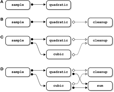
Figure 1. Examples of dependency graphs. In panel (A), the input file of the job quadratic is an output of the job sample; sample thus needs to be completed before starting quadratic. This type of dependency (“file-passing”) can be represented as a directed dependency graph. In panel (B), the job cleanup deletes an input file of quadratic; quadratic thus needs to be completed before starting cleanup. Note that such “cleanup” dependencies may involve more than two jobs: if cleanup deletes some input files used by both quadratic and cubic, cleanup depends on both of them (panel C). The same property holds for “file-passing” dependencies: if sum is using the outputs of both quadratic and cubic, sum depends on both jobs (panel D).
Let's now assume that the output of sample is regarded as an intermediate file that does not need to be retained. A new job cleanup is added to delete the output of sample, which is declared using the field files_clean:
% Adding a job "cleanup" : delete the

                   output of "sample"

pipeline.cleanup.command         =

            'delete(files_clean)';

pipeline.cleanup.files_clean  =

           pipeline.sample.files_out;
Because cleanup will delete the input file of quadratic, it is mandatory to wait until quadratic is successfully executed before cleanup is started. This type of dependency, called “cleanup”, is again included as a directed link in the dependency graph, see Figure 1B.
The order in which the jobs are added to the pipeline does not have any implications on the dependency graph, and is thus independent of the order of their execution. For example, if a new job cubic is added:
% Adding a job "cubic" : Compute a.^3 and

                         save the results

command = 'load(files_in);

           c = a.^3; save(files_out,''c'')';

pipeline.cubic.command    = command;

pipeline.cubic.files_in  =

              pipeline.sample.files_out;

pipeline.cubic.files_out  =

              'cubic.mat';
the job cleanup will be dependent upon quadratic and cubic, because the latter jobs are using the output of sample as an input, a file that is deleted by cleanup (Figure 1C).
The type of files_in, files_out, and files_clean is highly flexible. It can be a string, a cell of strings, or a nested structure whose terminal fields are strings or cells of strings. The following job for example uses two inputs, generated by two different jobs (see Figure 1D):
% Adding a job "sum" : Compute a.^2+a.^3

                    and save the results

command = 'load(files_in{1});

        load(files_in{2}); d = b+c, …

        save(files_out,''d'')';

pipeline.sum.command      = command;

pipeline.sum.files_in{1} =

          pipeline.quadratic.files_out;

pipeline.sum.files_in{2} =

          pipeline.cubic.files_out;

pipeline.sum.files_out   = 'sum.mat';
3. Pipeline Execution
3.1. A first Pass Through the Toy Pipeline
When a pipeline structure has been generated by the user, PSOM offers a generic command to execute the pipeline:
psom_run_pipeline(pipeline,opt_pipe)
where opt_pipe is a structure of options that can be used to set the configuration of PSOM, see Section 4.6. The main configuration option is the name of a folder used to store the logs of the pipeline, which is the “memory” of the pipeline system. When invoked, PSOM first determines which jobs need to be restarted using the logs folder. The jobs are then executed in independent sessions, as soon as all their dependencies are satisfied. The next section (Section 4) describes the implementation of all stages of pipeline execution in details. This section outlines the key mechanisms using simple examples, starting with the toy pipeline presented in the last section without the cleanup job (see Figure 2). Initially, only one job (sample) can be started because it does not have any parent in the dependency graph (Figure 2A). As soon as this job has been successfully completed, its two children (quadratic and cubic) are started. This is assuming of course that the configuration allows PSOM to execute at least two jobs in parallel (e.g., background execution on a dual-core machine), see Figure 2B. The job sum is started only when both of its dependencies have been satisfied, see Figures 2C,D. When all jobs are completed, the pipeline manager finally exits (Figure 2E).
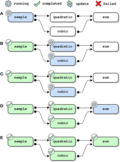
Figure 2. Pipeline execution: a first pass through the toy pipeline. Each panel represents one step in the execution of the toy pipeline presented in Section 2, without the cleanup job. This example assumes that at least two jobs can run in parallel, and that the pipeline was not executed before. All jobs are executed as soon as all of their dependencies are satisfied, possibly with some jobs running in parallel.
3.2. Updating a Pipeline (with a Bug)
This next example shows how the pipeline manager deals with the update of a pipeline. That is to say that a pipeline is submitted for execution after it was previously executed using the same logs folder. If one of the jobs has changed since the last submission, this job along with all of its children in the dependency graph are scheduled to be reprocessed. Here, the job quadratic is modified to introduce a bug, before restarting the pipeline:
% Changing the job quadratic to

  introduce a bug

pipeline.quadratic.command = 'BUG!';

% Restart the pipeline

psom_run_pipeline(pipeline,opt_pipe)
The pipeline manager first restarts the job quadratic because a change is detected in its description (Figure 3A). After the execution of the job is completed, the job is tagged with a “failed” status (panel B). The job sum is not started because it has a dependency that cannot be solved, and the pipeline manager simply exits. It is then possible to access the logs of the failed job, i.e., a text description of the job, start time, user name, system used as well as end time and all text outputs:
>> psom_pipeline_visu

    (opt.path_logs,'log','quadratic');

***********************************

Log of the (octave) job : quadratic

Started on 19-Jul-2011 16:01:36

User: pbellec

host : sorbier

system : unix

***********************************

command     = BUG!

files_in      = /home/pbellec/database/

              demo_psom/sample.mat

files_out   = /home/pbellec/database

              /demo_psom/quadratic.mat

files_clean = {}(0x0)

opt         = {}(0x0)

********************

The job starts now !

********************

Something went bad … the job has FAILED !

The last error message occured was :

parse error:

  syntax error

>>> BUG!

File /home/pbellec/svn/psom/trunk/

      psom_run_job.m at line 110

****************

Checking outputs

****************

The output file or directory …

   /home/pbellec/database/demo_psom/

  quadratic.mat has not been generated!


*******************************************

19-Jul-2011 16:01:36 : The job has FAILED

Total time used to process the

      job : 0.00 sec.

*******************************************
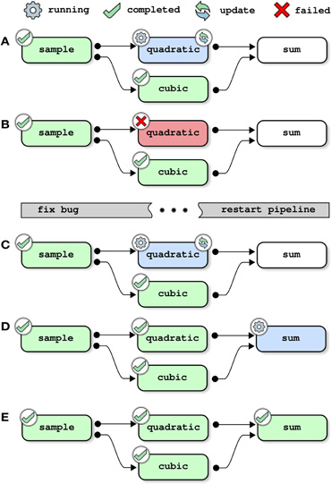
Figure 3. Pipeline management, example 2: updating a pipeline (with one bug). Each panel represents one step in the execution of the toy pipeline presented in Section 2, without the cleanup job. This example assumes that at least two jobs can run in parallel, and that the pipeline has already been executed once as outlined in Figure 2. The pipeline is first started after changing the job quadratic to introduce a bug (panels A–B). When the execution of the pipeline fails, the job quadratic is modified to fix the bug. The pipeline is then restarted and completes successfully (panels C–E).
The pipeline is then modified to fix the bug in quadratic. After restarting the pipeline, the jobs quadratic and sum run sequentially and are successfully completed (Figures 3C–E).
3.3. Adding a Job
Updating the pipeline is not solely restricted to changing the description of a job that was previously a part of the pipeline. It is also possible to add new jobs and resubmit the pipeline. Figure 4 shows the steps of resolution of the full toy pipeline (including the cleanup job) when the subpipeline (not including the clean-up pipeline) had already been successfully completed prior to submission. In that case, there is no job that depends on the outputs of cleanup, so the only job that needs to be processed is cleanup itself and the pipeline is successfully completed immediately after this job is finished.
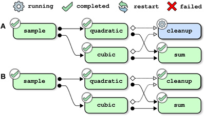
Figure 4. Pipeline management, example 3: adding a (cleanup) job. This example assumes that the toy pipeline (without the cleanup job) had already been successfully completed. The full toy pipeline (with the cleanup job) is then submitted for execution. The only job that is not yet processed is cleanup, and the pipeline execution ends after cleanup successfully completes.
3.4. Restarting a Job After Clean Up
It is sometimes useful to force a job to restart, for example a job that executes a modified script while the job description remains identical. PSOM is not able to detect this type of change in the pipeline (it assumes that all libraries are identical across multiple runs of the pipeline). The following option will force a job to restart:
opt_pipe.restart = {'quadratic'};

psom_run_pipeline(pipeline,opt_pipe);
In this example, all jobs whose name includes quadratic will be restarted by the pipeline manager. Further we will assume that the full toy pipeline (including the cleanup job) has already been completed. In the absence of the cleanup job, the job quadratic would be restarted as well as all of its children. The inputs of quadratic, however, have been deleted by cleanup. It is therefore, not possible to restart the pipeline at this stage. The pipeline manager will automatically detect that the missing inputs can be re-generated by restarting the job sample. It will thus restart this job as well as all of its children, including cubic (see Figure 5 for a step-by-step resolution of the pipeline). Note that this behavior is iterative, such that if some inputs from sample had been missing, the pipeline manager would look for jobs that could be restarted to generate those files.
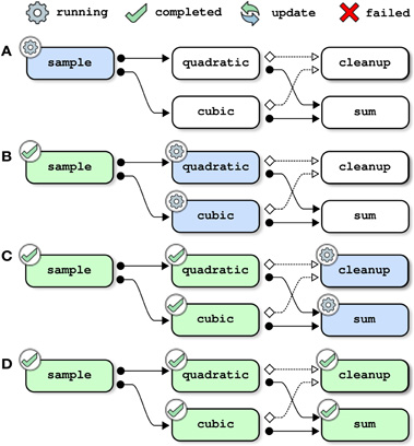
Figure 5. Pipeline management, example 4: restarting a job after its inputs have been cleaned up. This example assumes that the full toy pipeline (including the cleanup job) has already been successfully completed. The same pipeline is then submitted for a new run and the job quadratic is forced to be restarted. Because the inputs of quadratic (generated by sample) have been deleted by cleanup, the pipeline manager also restarts the job sample (panel A). Because all jobs depend indirectly on sample, all jobs in the pipeline have to be reprocessed (panels B–D).
3.5. Pipeline History
When PSOM is solving a pipeline, it is not generating a color-coded graph such as those presented in Figures 2–5. Rather, it outputs a text summary of all operations, such as job submission, job completion, and job failure. Each event is reported along with the time of its occurrence. This is presented in the following example for the first execution of the toy pipeline (Figure 2):
*****************************************

The pipeline PIPE is now being processed.

Started on 21-Jul-2011 09:37:45

user: pbellec, host: berry, system: unix

*****************************************

21-Jul-2011 09:37:45 -

…The job sample has been submitted to the

 queue (1 jobs in queue).

21-Jul-2011 09:37:48 -

…The job sample has been successfully

 completed (0 jobs in queue).

21-Jul-2011 09:37:48 -

…The job quadratic has been submitted to

 the queue (1 jobs in queue).

21-Jul-2011 09:37:48 -

…The job cubic has been submitted to the

 queue (2 jobs in queue).

21-Jul-2011 09:37:52 -

…The job quadratic has been successfully

 completed (1 jobs in queue).

21-Jul-2011 09:37:52 -

…The job cubic has been successfully

 completed (0 jobs in queue).

21-Jul-2011 09:37:52 -

…The job sum has been submitted to the

 queue (1 jobs in queue).

21-Jul-2011 09:37:55 -

…The job sum has been successfully

 completed (0 jobs in queue).

*******************************************

The processing of the pipeline is

terminated.

See report below for job completion status.

21-Jul-2011 09:37:55

*******************************************

All jobs have been successfully completed.
These logs are concatenated across all instances of pipeline executions, and they are saved in the logs folder. They can be accessed using a dedicated M-command:
psom_pipeline_visu

   (opt_pipe.path_logs,'monitor')
The logs of individual jobs can also be accessed with the same command, using a different option:
psom_pipeline_visu

   (opt_pipe.path_logs,'log',JOB_NAME)
as shown in Section 3.2. Finally, it is possible to get access to the execution time for all jobs from the pipeline, which can be useful for benchmarking purposes:
>> psom_pipeline_visu

   (opt_pipe.path_logs,'time','')

**********

cleanup     : 0.07 s, 0.00 mn,

            0.00 hours, 0.00 days.

cubic       : 0.07 s, 0.00 mn,

            0.00 hours, 0.00 days.

quadratic : 0.08 s, 0.00 mn,

            0.00 hours, 0.00 days.

sample       : 0.13 s, 0.00 mn,

            0.00 hours, 0.00 days.

sum       : 0.11 s, 0.00 mn,

            0.00 hours, 0.00 days.

**********

Total computation time :  0.46 s, 0.01 mn,

                   0.00 hours, 0.00 days.
4. Implementation of the Pipeline Execution Engine
4.1. Overview
At the user level, PSOM requires two objects to be specified: (1) a pipeline structure which describes the jobs, see Section 2; (2) an opt_pipe structure which configures how the jobs will be executed, see Section 4.6. The configuration notably includes the name of a so-called logs folder, where a comprehensive record of the pipeline execution is kept. The pipeline execution itself is initiated by a call to the function psom_run_pipeline, which comprises three distinct modules:
- The initialization stage starts off with basic viability checks. If the same logs folder is used multiple times, the current pipeline is compared against older records. This determines which jobs need to be (re)started.
- When the initialization stage is finished, a process called the pipeline manager is started. The pipeline manager remains active as long as the pipeline is running. Its role is to create small scripts to run individual jobs, and then submit those scripts for execution as soon as their dependencies are satisfied and sufficient resources, as determined by the configuration, become available.
- Each job is executed in an independent session by a job manager. Upon termination of the job, the completion status (“failed” or “finished”) is checked and reported to the pipeline manager using a “tag file” mechanism.
This section describes the implementation of each module, as well as the configuration of PSOM and the content of the logs folder. An overview is presented in Figure 6.
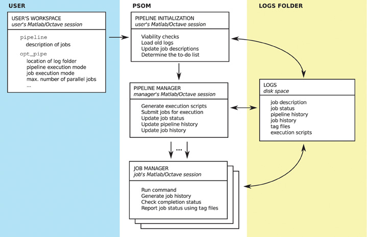
Figure 6. Overview of the PSOM implementation. On the user's side (left panel), a structure pipeline is built to describe the list of jobs, and a structure opt_pipe is used to configure PSOM. The memory of the pipeline is a logs folder located on the disk space (right panel), in which a series of files are stored to provide a comprehensive record of multiple runs of pipeline execution. The PSOM proceeds in three stages (center panel). At the initialization stage, the current pipeline is compared with previous executions to set up a “to-do” list of jobs that needs to be (re)started. Then, the pipeline manager is started, which constantly submits jobs for execution and monitors the status of on-going jobs. Finally, each job is executed independently by a job manager which reports the completion status upon termination (either “failed” or “finished”).
4.2. Pipeline Initialization
The initialization of pipeline execution includes the following steps:
- Check that the (directed) dependency graph of the pipeline is acyclic. A dependency graph that includes a cycle is impossible to solve.
- Check that all of the output files are generated only once (otherwise the results of the pipeline may depend on an arbitrary order of job executions).
- If available, retrieve the history of previous pipeline executions. Determine which jobs need to be processed based on the history. Update the pipeline history accordingly. This step will be further detailed below.
- Check that all of the input files that are not generated as part of the pipeline are present on the disk. If not, issue a warning because some jobs may fail when input files are missing. This, however, depends on the behavior of the commands specified by the user and cannot be tested by PSOM. The decision to continue is thus left to the user who may decide to interrupt the execution at this stage.
- Create all the necessary folders for output files. This feature circumvents the repetitive task of coding the creation of the output folder(s) inside each individual job.
- If some of the output files already exist, delete them. This step is intended to avoid possible errors in the pipeline execution due to some jobs not overwriting the output files.
To determine what jobs from the pipeline actually need to be processed, the jobs submitted for execution are compared with those previously executed in the same logs folder (if any), along with their completion status. There are three possible status results:
’none’means that the job has never been started (this is the default if no previous status exists).’finished’means that the job was previously executed and successfully completed.’failed’means that the job was previously executed and had failed.
A job will be added to the “to-do list” (i.e., will be executed by the pipeline manager) if it meets one of the following conditions:
- the job has a
’failed’status. - the job has a
’none’status. - the description of the job has changed.
- the user forced a restart of the job using
opt_pipe.restart. See Section 3.4.
Every time a job A is added to the to-do list, the following actions are taken:
- Change the status of the job
Ato’none’. - Add all jobs with a dependency on
Ato the “to-do list”. - If an input file of
Ais missing and a job of the pipeline can generate this file, add this last job to the “to-do list”.
Note that the process of adding a job to the to-do list is recursive and it can lead to restarting a job with a ’finished’ status, e.g., if that job has changed or if it is dependent on a job that has changed.
4.3. Pipeline Manager
After the pipeline has been initialized, a small process called the “pipeline manager” is started. The pipeline manager is essentially a long loop that constantly monitors the state of the pipeline, and submits jobs for execution. The pipeline manager as well as the individual jobs can run within the current O/M session, or in an independent session running either locally (on the same machine) or remotely (on another computer/node). At any given point in time, the pipeline manager submits all of the jobs that do not have an unsatisfied dependency, as long as there are enough resources available to process the jobs. The following rules apply to determine if the dependencies of a job are satisfied:
- If a job has been successfully completed, the dependencies to all the children in the dependency graph are considered satisfied.
- Conversely, the dependencies of a job are all satisfied if there are no dependencies in the first place or if the parents in the dependency graph all have a
’finished’status.
Depending on the selected configuration, there may also be a limit to the maximal number of jobs that can be submitted for execution simultaneously. This was implemented because some high-performance computing facilities impose such a limit. Upon completion or failure, the jobs report their status using tag files located in the logs folder. A tag file is an empty file with a name of the form JOB_NAME.failed or JOB_NAME.finished, which indicates the completion status. If the pipeline system was fully based on tag files to store status, a pipeline with thousands of jobs would create thousands of tag files. This would cause very important delays when accessing the file system. The pipeline manager thus monitors these tag files and removes them as soon as their presence is detected. The tag files are used to update a single O/M file coding for the status of all jobs in the pipeline. As the tag files are empty files, there is no possible race condition between their creation and their subsequent removal by the pipeline manager. The pipeline manager also adds status updates in a plain text “history” file which can be monitored while being updated in a terminal or from O/M through the dedicated command psom_pipeline_visu.
4.4. Job Manager
When a job is submitted for execution by the pipeline manager, the command specified by the user is always executed by a generic job manager. The job manager is a matlab function (psom_run_job) which automates the generation of a job profile, logs, as well as the tag files that are used to report the completion status to the pipeline manager. This function notably executes the command in a try… catch block, which means that errors in the command will not crash the job manager. When the command has finished to run, the job manager will check that all of the output files have been properly generated. If an error occurs, or if one of the output files is missing, then the job is marked as ’failed’. Otherwise it is considered ’finished’. The job manager reports back the completion status of the job to the pipeline manager using a tag file mechanism already described in Section 4.3. The job manager also automatically generates logs, i.e., a text record of the execution of the command, as well as other automatically generated informations such as the user name, the date, the time, and the type of operating system, see Section 3.5 for an example. Finally, the job manager measures and saves the execution time of the command for profiling purposes.
4.5. Logs Folder
The logs folder contain the following files:
PIPE_history.txt: A plain text file with the history of the execution of the pipeline manager (see Section 3.5 for an example).PIPE_jobs.mat: An O/M file were each job is saved as a variable. This structure includes the latest version of all jobs executed from the logs folder.PIPE_status.mat: An O/M file where the status of each job is saved as one (string) variable.PIPE_logs.mat: An O/M file where the logs of each job is saved as one (string) variable.PIPE_profile.mat: An O/M file where each job appears as a variable. This variable is an O/M structure, notably including the execution time of the command.PIPE.mat: An O/M file where PSOM configuration variables are saved.
Importantly, using PIPE_jobs.mat, it is possible to re-execute the pipeline from scratch at any point in time, or to access any of the parameters that were used for the analysis. The logs folder thus contains enough information to fully reproduce the results of the pipeline. Moreover, with this information being stored in the form of an M-structure, it is easy to access and fully scalable. This can support jobs with potentially hundreds or even thousands of parameters. Octave and Matlab both use the HDF5 file format (Poinot, 2010). This format offers internal compression, yet still allows PSOM to read or write individual variables without accessing the rest of the file. This is a key technical feature that enables PSOM to quickly update the logs/status/profile files for each job, regardless of the size of the pipeline. Note that the logs folder also contain other files generated temporarily as part of the pipeline submission/execution process, as well as backup files in the event the main files are corrupted.
4.6. PSOM Configuration
The only necessary option to start a pipeline is setting where to store the logs folder:
>> opt_pipe.path_logs =

  '/home/pbellec/database/demo_psom/logs/';
It is highly recommended that the logs folder be used solely for the purposes of storing the history of the pipeline. Another important, yet optional parameter is setting how the individual jobs of the pipeline are executed:
>> opt_pipe.mode = 'batch';
Five execution modes are available:
’session’: The jobs are executed in the current O/M session, one after the other.’background’: This is the default. Each job is executed in the background as an independent O/M session, using an “asynchronous” system call. If the user's session is interrupted, the pipeline manager and the jobs are interrupted as well.’batch’: Each job is executed in the background as an independent O/M session, using theatcommand on Linux and thestartcommand on windows. If the user's session is interrupted, the pipeline manager and the jobs are not interrupted. This mode is less robust thanbackgroundand may not be available on some platforms.’qsub’: The jobs are executed on a remote execution server through independent submissions to a queuing scheduler using aqsubcommand (either torque, SGE, or PBS). Such queuing schedulers are in general avalaible in high-performance computing facilities. They need to be installed and configured by a system administrator.’msub’: The jobs are executed on a remote execution server through independent submissions to a a queuing scheduler using amsubcommand (MOAB). This is essentially equivalent to theqsubmode.
Additional options are available to control the bash environment variables, as well as O/M start-up options, among others. A function called psom_config can be used to assess whether the configuration of PSOM is correct. This procedure includes multiple tests to validate that each stage of a job submission is working properly. It will provide some environment-specific suggestions to fix the configuration when a problem is detected. PSOM release 0.9 has been tested in a variety of platforms (Linux, windows, Mac OSX) and execution modes. More details can be found in PSOM online resources, see the discussion section for links.
5. Coding Guidelines for Modules and Pipelines
The pipeline structure that is used in PSOM is very flexible, as it does not impose any constraints on the way the code executed by each job is implemented or on the way the pipeline structure itself is generated. Additional coding guidelines and tools have been developed to keep the code concise and scalable, in the sense that it can be used to deal with functions with tens or hundreds of parameters and thousands of jobs. These guidelines also facilitate the combination of multiple pipelines while keeping track of all parameters: a critical feature to ensure full provenance of a pipeline analysis. A generic tool is available to test the presence of mandatory parameters and set up default parameter values. Another tool is the so-called “brick” function type, which can be used to run jobs. A last set of guidelines and tools have been developed to generate the pipeline structures themselves.
5.1. Setting the Job Parameters
There is no strict framework to set the default of the input arguments in Octave/Matlab. We developed our own guidelines, which have several advantages over a more traditional method consisting in passing each parameter one by one. As can be seen in the attributes of a job, our method consists of passing all parameters as fields of a single structure opt. A generic function psom_struct_defaults can be used to check for the presence of mandatory input arguments, set default values, and issue warnings for unkown arguments. The following example shows how to set the input arguments of a function using that approach:
opt.order     = [1 3 5 2 4 6];

opt.slic        = 1;

opt.timing      = [0.2,0.2];

list_fields      = { 'method' , 'order' ,

         'slice' , 'timing' , 'verb' };

list_defaults = { 'linear' , NaN     , []     ,

                   NaN      , true   };

opt = psom_struct_defaults

      (opt,list_fields,list_defaults)

warning: The following field(s)  were

    ignored in the structure :  slic

opt = {

   method = linear

   order   =  [1   3   5   2   4   6]

   slice   = [](0x0)

   timing = [0.20000   0.20000]

   verb     =  1 }
Note that only three lines of code are used to set all the defaults, and that a warning was automatically issued for the typo slic instead of slice. Such unlisted fields are simply ignored. Also, the default value NaN can be used to indicate a mandatory argument (an error will be issued if this field is absent). This approach will scale up well with a large number of parameters. It also facilitates the addition of extra parameters in future developments while maintaining backwards compatibility. As long as a new parameter is optional, a code written for old specifications will remain functional.
5.2. Building Modules for a Pipeline : the “Brick” Function Type
The bricks are a special type of O/M function which take files as inputs and outputs, along with a structure to describe some options. In brief, a brick precisely mimics the structure of a job in a pipeline, except for the files_clean field. The command used to call a brick always follows the same syntax:
[files_in,files_out,opt] =

   brick_name(files_in,files_out,opt)
where files_in, files_out and opt play the same roles as the fields of a job. The key mechanism of a brick is that there will always be an option called opt.flag_test which allows the programmer to make a test, or dry-run. If that (boolean) option is true, the brick will not do anything but update the default parameters and file names in its three arguments. Using this mechanism, it is possible to use the brick itself to generate an exhaustive list of the brick parameters, and test if a subset of parameters are acceptable to run the brick. In addition, if a change is made to the default parameters of a brick, this change will be apparent to any piece of code that is using a test to set the parameters, without a need to change the code.
When the file names files_in or files_out are structures, a missing field will be interpreted either as a missing input which can be replaced by a default dataset, or an output that does not need to be generated. If the field is present but empty, then a default file name is generated. Note that an option opt.folder_out can generally be used to specify in which folder the default outputs should be generated. Finally, if a field is present and non-empty, the file names specified by the users are used to generate the outputs. These conventions allow complete control over the number of output files generated by the brick, and the flexibility to use default names. The following example is a dry-run with a real brick implemented in the neuroimaging analysis kit17 (NIAK) (Bellec et al., 2011):
files_in  =

   '/database/func_motor_subject1.mnc';

files_out.filtered_data = '';

files_out.var_low = '';

opt.hp = 0.01;

opt.folder_out = '/database/filtered_data/';

opt.flag_test = true;

>>[files_in,files_out,opt] = … niak_brick

        _time_filter(files_in,files_out,opt)

files_in  =

     /database/func_motor_subject1.mnc

files_out =

{

 filtered_data = /database/filtered_data/

            /func_motor_subject1_f.mnc

 var_high           = gb_niak_omitted

 var_low             = /database/filtered

    _data//func_motor_subject1_var_low.mnc

 beta_high         = gb_niak_omitted

 beta_low           = gb_niak_omitted

 dc_high             = gb_niak_omitted

 dc_low               = gb_niak_omitted

}

opt =

{

 hp                       =  0.010000

 folder_out       = /database/filtered_data/

 flag_test         =  1

 flag_mean         =  1

 flag_verbose   =  1

 tr             = -Inf

 lp            = Inf

}
The default output names have been generated in opt.folder_out, and some of the outputs will not be generated (they are associated with the special tag ’gb_niak_omitted’). A large number of other parameters that were not used in the call have been assigned some default values.
5.3. Pipeline Implementation
A so-called pipeline generator is a function that, starting from a minimal description of a file collection and some options, generates a full pipeline. Because a pipeline can potentially create a very large number of outputs, it is difficult to implement a generic system that is as flexible as a brick in terms of output selection. Instead, the organization of the output of the pipeline will follow some canonical, well-structured pre-defined organization. As a consequence, the pipeline generator only takes two input arguments, files_in and opt (similar to those of a job), and does not feature files_out. The following example shows how to set files_in for niak_pipeline_corsica, implemented in NIAK:
%% Subject 1

files_in.subject1.fmri{1} =

   '/demo_niak/func_motor_subject1.mnc';

files_in.subject1.fmri{2} =

   '/demo_niak/func_rest_subject1.mnc';

files_in.subject1.transf  =

   '/demo_niak/transf_subject1.xfm';


%% Subject 2

files_in.subject2.fmri{1} =

   '/demo_niak/func_motor_subject2.mnc';

files_in.subject2.fmri{2} =

   '/demo_niak/func_rest_subject2.mnc';

files_in.subject2.transf  =

   '/demo_niak/transf_subject2.xfm';
The argument opt will include the following standard fields:
opt.folder_out: Name of the folder where the outputs of the pipeline will be generated (possibly organized into subfolders).opt.size_output: This parameter can be used to vary the amount of outputs generated by the pipeline (e.g.,’all’: generate all possible outputs;’minimum’, clean all intermediate outputs, etc).opt.brick1: All the parameters of the first brick used in the pipeline.opt.brick2: All the parameters of the second brick used in the pipeline.- …
Inside the code of the pipeline template, adding a job to the pipeline will typically involve a loop similar to the following example:
% Initialize the pipeline to a structure

  with no field

pipeline = struct();

% Get the list of subjects from files_in

list_subject = fieldnames(files_in);

% Loop over subjects

for num_s = 1:length(list_subject)

    % Plug the 'fmri' input files of the

      subjects in the job

    job_in  = files_in.

            (list_subject{num_s}).fmri;

    % Use the default output name

    job_out = '';

    % Force a specific folder organization

      for outputs

    opt.fmri.folder_out = [opt.folder_out

            list_subject{num_s} filesep];

    % Give a name to the jobs

    job_name =

       ['fmri_' list_subject{num_s}];

    % The name of the employed brick

    brick = 'brick_fmri';

    % Add the job to the pipeline

    pipeline = … psom_add_job(pipeline,

    job_name,brick,job_in,job_out,opt.fmri);

    % The outputs of this brick are just

      intermediate outputs :

    % clean these up as soon as possible

    pipeline = psom_add_clean(pipeline,

           [job_name … '_clean'],pipeline.

           (job_name).files_out);

end
The command psom_add_job first runs a test with the brick to update the default parameters and file names, and then adds the job with the updated input/output files and options. By virtue of the “test” mechanism, the brick is itself defining all the defaults. The coder of the pipeline does not actually need to know which parameters are used by the brick. Any modification made to a brick will immediately propagate to all pipelines, without changing one line in the pipeline generator. Moreover, if a mandatory parameter has been omitted by the user, or if a parameter name is not correct, an appropriate error or warning will be generated at this stage, prior to any work actually being performed by the brick. The command psom_add_clean adds a cleanup job to the pipeline, which deletes the specified list of files. Because the jobs can be specified in any order, it is possible to add a job and its associated cleanup at the same time. Finally, it is very simple to combine pipelines together: the command psom_merge_pipeline simply combines the fields of two structures pipeline1 and pipeline2.
6. Applications in Neuroimaging
The PSOM project is just reaching the end of its beta testing phase, and as such it has only been adopted by a couple of laboratories as a development framework. There are still been several successful applications, including the generation of simulated fMRI (Bellec et al., 2009), clustering in resting-state fMRI (Bellec et al., 2010a, b), clustering in event-related fMRI (Orban et al., 2011), simulations in electroencephalography and optical imaging (Machado et al., 2011), reconstruction of fiber tracts (Kassis et al., 2011), as well as non-parametric permutation testing (Ganjavi et al., 2011). The PSOM framework has also been used for the development of an open-source software package called NIAK18 (Bellec et al., 2011). This software package, which relies on the PSOM execution engine, has been used in a number of recent studies (Dansereau et al., 2011; Moeller et al., 2011; Schoemaker et al., 2011; Carbonell et al., 2012). We used the fMRI preprocessing pipeline from the NIAK package to run benchmarks of the parallelization efficiency of the PSOM execution engine. This pipeline has been integrated into the CBRAIN computing platform (Frisoni et al., 2011), where it has been used to preprocess and publicly release19 fMRI datasets collected for about 1000 children and adolescents, as part of the ADHD-200 initiative20 (Lavoie-Courchesne et al., 2012).
6.1. The NIAK fMRI Preprocessing Pipeline
The NIAK fMRI preprocessing pipeline applies the following operations to each functional and structural dataset in a database. The first 10 s of the acquisition are suppressed to allow the magnetization to reach equilibrium. The fMRI volumes are then corrected of inter-slice difference in acquisition time, rigid body motion, slow time drifts, and physiological noise (Perlbarg et al., 2007). For each subject, the mean motion-corrected volume of all the datasets is coregistered with a T1 individual scan using minctracc (Collins et al., 1994), which is itself non-linearly transformed to the Montreal Neurological Institute (MNI) non-linear template (Fonov et al., 2011) using the CIVET pipeline (Ad-Dab'bagh et al., 2006). The functional volumes are then re-sampled in the stereotaxic space and spatially smoothed.
Most operations are implemented through generic medical image processing modules, the MINC tools21. These tools are coded in a mixture of C and C++ languages, as well as some PERL scripts, and usually operate through the command line. Simple PSOM-compliant “brick” wrappers have been implemented in NIAK for the required MINC tools. Other bricks are also pure O/M implementations for original methods or a port from other O/M projects. Finally, some of the operations (motion correction, correction of physiological noise) are themselves pipelines involving several steps, see Figure 7 for an example of a full dependency graph. The code of the individual NIAK fMRI preprocessing pipeline is 735 lines long, and only 321 lines after excluding header comments and variable initialization. The code is thus concise enough to be easily reviewed, quality-checked, and modified.
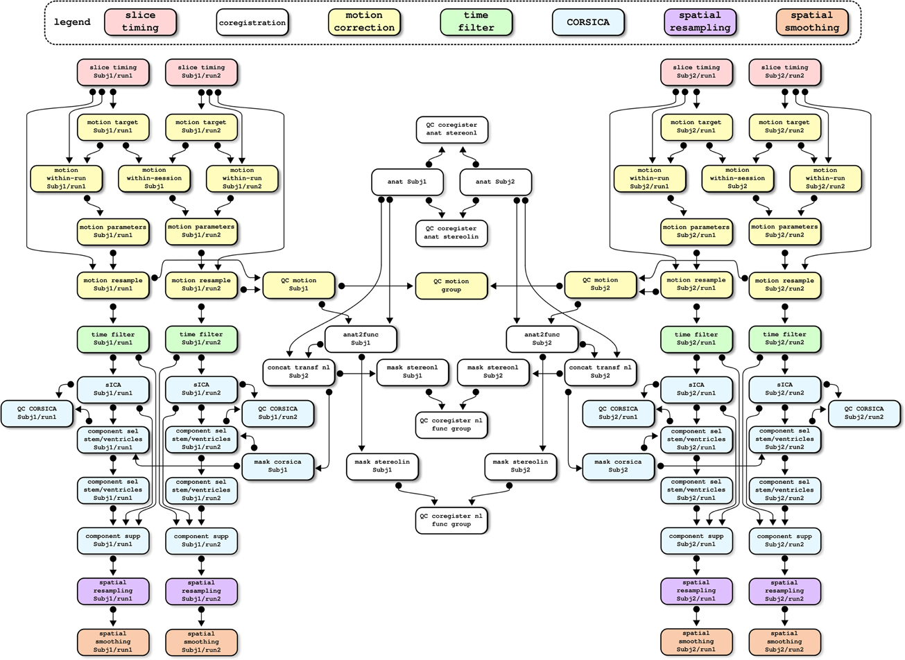
Figure 7. An example of dependency graph for the NIAK fMRI preprocessing pipeline. This example includes two subjects with two fMRI datasets each. The pipeline includes close to 100 jobs, and cleanup jobs have been removed to simplify the represen-tation. Colors have been used to code the main stages of the preprocessing.
6.2. Benchmarks
We used the Cambridge resting-state fMRI database for the benchmark, which is publicly available as part of the 1000 functional connectome project22. This database (Liu et al., 2009) includes 198 subjects with one structural MRI and one fMRI run each (119 volumes, TR = 3 s). The processing was done in various computing environments and execution modes to test the scalability of PSOM:
peuplier-n: A machine with an Intel(R) Core™ i7 CPU (four computing cores, eight threads), 16 GB of memory, a local file system and an Ubuntu operating system. For n =1, both the pipeline manager and individual jobs were executed sequentially in a single Octave session. For n > 1, the pipeline manager and individual jobs were executed in the background in independent Octave sessions using anatcommand, with up tonjobs running in parallel.magma-n: a machine with four six-Core AMD Opteron™ Processor 8431 (for a total of 24 computing cores), 64 GB of memory, an NTFS mounted file system and an openSUSE operating system. Forn=1, both the pipeline manager and individual jobs were executed sequentially in a single Octave session. Forn>1, the pipeline manager ran in the background using anatcommand and individual jobs were executed in the background in independent Octave sessions using an SGEqsubcommand, with up tonjobs running in parallel.guillimin-n: a supercomputer with 14400 Intel Westmere-EP cores distributed across 1200 compute nodes located at the CLUMEQ-McGill data centre, Ecole de Technologie Superieure in Montreal, Canada.guilliminranked 83th in the top 500 list of the most powerful supercomputers, released in November, 201123. Included in the facility is nearly 2 PB of disk storage using the general parallel file system (GPFS). Forn=1, both the pipeline manager and individual jobs were executed sequentially in a single Octave session. Forn>1, the pipeline manager ran in the background using anatcommand and individual jobs were executed on distributed computing nodes in independent Octave sessions using a MOABmsubcommand, with up tonjobs running in parallel.
We investigated the performance of PSOM on (peuplier-8, magma-{8,16,24,40} and guillimin-{24,50,100,200}). For experiments on peuplier and magma, Octave release 3.2.4 was used, with PSOM release 0.8.9 and NIAK release 0.6.4.3. On guillimin, octave release 3.4.2 was available and some development versions of NIAK (v1270 on the subversion repository) and PSOM (v656 of the subversion repository) were used because they implemented some bug fix for this release. During the time of the experiment, the PSOM jobs were the only ones running on the execution servers for peuplier and magma, while guillimin had about 75% processors in use.
6.3. Results
The raw Cambridge database had a size of 7.7 GB, with a total of 21 GB generated by the pipeline (output/input ratio of 273%). The NIAK pipeline included 5153 jobs featuring 8348 unique input/output files (not including temporary files). Figure 8A shows the distribution of execution times for all jobs on peuplier-8. The pipeline included about 1500 “cleanup” jobs deleting intermediate files, with an execution time of less than 0.2 s. The other jobs lasted anywhere between a few seconds and 15 min, with hundreds of jobs of less than 2 min. Because of the large number of very short jobs, the pipeline manager was not able to constantly submit enough jobs to use n cores at all time, even when it would have been possible in theory. This effect was small on peuplier, magma or guillimin-{24,50} see Figure 8B–C. It became pronounced on guillimin-{100,200}, see Figure 8D. The serial execution time of the pipeline (sum of execution time of all jobs) varied a lot from one configuration to the other: from 120 h (5 days) on guillimin-24 to almost double (220 h, 9 days) on magma-8. The serial execution time, however, increased quickly on guillimin with an increasing n, see Figure 8E. Despite this effect, and thanks to parallelization, the parallel execution time (time elapsed between the beginning and the end of the pipeline processing) steadily decreased with an increasing n, see Figure 8F. The speed-up factor (defined as the ratio between the serial and parallel execution time) still departed from the optimal value n. Consistent with our observations on the effective number of cores used on average, the departure between the speed-up factor and n increased with n, and became pronounced for n greater than 100, see Figure 8G. This result can be expressed as a parallelization efficiency, defined as the ratio between the empirical speed-up factor and n. Parallelization efficiency was excellent (over 90%) on peuplier-8 and gradually decreased with an increasing n to reach about 80% on peuplier-24 or guillimin-24 and 60% on guillimin-200. In this last setting, the fMRI datasets and structural scans of about 200 subjects were still processed in a little bit more than 2 h.
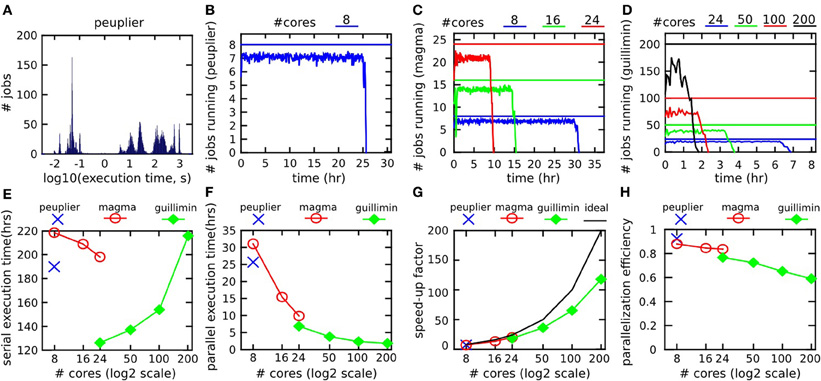
Figure 8. Benchmark experiments with the NIAK fMRI preprocessing pipeline. The distribution of execution time for all jobs on one server (peuplier) is shown in panel (A). The number of jobs running at any given time across the whole execution of the pipeline (averaged on 5 min time windows) is shown in panels (B–D) for servers peuplier, magma and guillimin, respectively. The user-specified maximum number of concurrent jobs is indicated by a straight line. The serial execution time of the pipeline, i.e., the sum of execution times for all jobs, is shown in panel (E). The parallel execution time, i.e., the time elapsed between the beginning and the end of the pipeline processing, is shown in panel (F). The speed-up factor, i.e., serial time divided by parallel time, is presented in panel (G), along with the ideal speed-up, equal to the user-specified maximal number of concurrent jobs. Finally, the parallelization efficiency (i.e., the ratio between the empirical speed-up and the ideal speed-up) is presented in panel (H).
7. Discussion
7.1. Overview
We propose a new PSOM to implement, run, and re-run pipeline analysis on large databases. Our approach is well-suited for pipelines involving heterogeneous tools that can communicate through a file system in a largely parallel fashion. This notably matches the constraints found in neuroimaging. The PSOM coding standards produce concise, readable code which in our experience is easy to maintain and develop over time. It is also highly scalable: a pipeline can incorporate thousands of jobs, each one featuring tens to hundreds of parameters. From a developer's perspective, using PSOM does not limit the scope of distribution of the software, as pipelines can be executed inside an O/M session as would any regular O/M code. The very same code can also be deployed on a multi-core machine or in a supercomputing environment simply by changing the PSOM configuration.
7.2. Online Documentation
The main body of documentation is available on a wiki hosted online by google code, see Table 1. This resource is updated for each new release of PSOM. It covers selected topics such as the configuration of the pipeline manager more extensively than this paper. The “short PSOM tutorial” reproduces step-by-step all the experiments reported in Section 3.
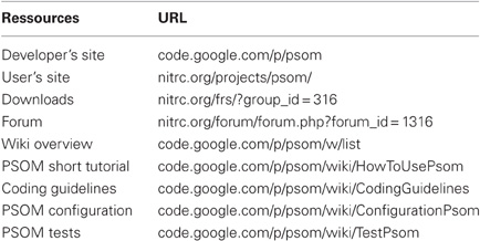
Table 1. Online resources for PSOM.
7.3. The Benefits of Pipeline Analysis
Parallel computing is a central feature of PSOM, as it allows to reduce the time necessary to complete an analysis. The pipeline system can be beneficial even when used within a single session. PSOM automatically keeps a record of all the steps and parameters of the pipeline. These logs are detailed enough to reproduce an entire analysis (as long as the production environment itself can be reproduced). This is an essential feature in the perspective of reproducible research. The pipeline logs can also be used for profiling the execution time of the whole pipeline as well as its subparts. This can be useful to run a benchmark or to identify computational bottlenecks. It is finally possible to restart the pipeline at any stage, or even to add stages or change parameters. Over multiple executions, PSOM will restart only the pipeline stages impacted by the changes. This ability to properly handle pipeline updates is critical in the development phase, and can also be useful to test alternative choices of parameter/algorithmic selection.
7.4. Parallel Computation Capabilities
The benchmark experiments demonstrated that PSOM is able to handle pipelines featuring thousands of jobs and tens of gigabytes of data. It can also dramatically reduce the execution time: an fMRI database including almost 200 subjects could be pre-processed in less than 3 h. The parallelization efficiency was excellent with a small or moderate number of computing cores (under 50), yet it dropped past a hundred cores. This is because the NIAK pipeline features hundreds of very short jobs (less than 0.2 s). The pipeline manager thus needs to submit jobs at a very high pace to use all resources. PSOM would behave better with longer jobs. Some alternative pipeline systems, e.g., Swift (Stef-Praun et al., 2007), scale efficiently up to thousands of cores even with short jobs (30 s long). Swift implements for this purpose a multi-level pipeline execution engine: the jobs are grouped into small sub-pipelines that are then processed independently. We are planning to add this feature to the pipeline execution engine in the next major release of PSOM.
7.5. Quality Control
Quality control is a challenge when processing large databases. This step is, however, critical to establish the scientific credibility of the results. Quality control is too problem-specific to be implemented as a general tool in a pipeline system. It is, however, possible to integrate ad-hoc steps of quality control in a pipeline. The NIAK fMRI preprocessing pipeline for instance includes a group summary of the individual motion parameters as well as measures of the quality of coregistration between the structural and functional images, amongst others. This approach was found to greatly facilitate the quality control of the preprocessing of ADHD-20024, a database including close to 1000 subjects (Lavoie-Courchesne et al., 2012).
7.6. Files Collection
Neuroimaging datasets often come as collections of files. The DICOM format for example may store individual slices as separate files. A variant of the NIFTI format (used by the SPM software) stores each brain volume of an fMRI dataset as one or two separate files. As hundreds of fMRI brain volumes are typically collected on an individual, both formats represent a large file collection. The structures used to describe input/output files in PSOM is very versatile, and can include an extensive file collection. There are, however, performance penalties for doing so. Those penalties are in part internal to PSOM, because analyzing the dependencies with DICOM or 3D NIFTI will take tens of seconds. Some operations on the file system may also slow down because of the number of files, independently of their size. This can be observed for example during the internet synchronization of file collections between sites. By contrast with the DICOM and 3D NIFTI formats, MINC or NIFTI have the ability to store a full 3D+t dataset into a single file. For computational efficiency, it is thus advisable to start a pipeline by converting the input database into such a 3D+t format.
7.7. PSOM Configuration
An important choice was made in the design of PSOM: the interactions between the pipeline manager and the execution controler (at, qsub, msub, etc.) are kept to a bare minimum. The main benefit of this approach is the ability of PSOM to interact easily and robustly with a variety of execution environments for the jobs. However, when a queuing scheduler is employed, PSOM has no means to interrogate the state of a particular job. It assumes that submitted jobs will be able to run, and if that assumption is met, each job will report its completion status using a file-based mechanism internal to PSOM. If this assumption is not met, the users may not get any useful feedback on the cause of failures. For this reason, a dedicated psom_config function is available to test each stage of job submission one by one, and will guide users when setting up their configuration.
7.8. Dynamic Pipeline Composition
In its current form, PSOM supports pipelines that can be described as a static DAG. Static means that the full pipeline representation has to be generated by the user prior to execution. In alternative pipeline systems such as Taverna, a pipeline can branch or iterate depending on data-dependent conditions that are dynamically evaluated during the execution. This is not currently possible in PSOM. A future development will address this issue by allowing jobs to regenerate themselves new jobs. This will be achieved by writing a description of these new jobs in a dedicated folder constantly monitored by the pipeline manager. This generic mechanism will enable a dynamic, data-dependent composition of the pipeline.
7.9. Interoperability
The PSOM framework fosters a modular organization of the code that is well adapted to a specific pipeline. Such organization will facilitate the subsequent implementation of the pipeline in any workflow system. Porting a pipeline from PSOM to another system may even become a largely automated task. We recently demonstrated the feasibility of this approach by building an interface between the NIAK fMRI preprocessing pipeline and CBRAIN (Lavoie-Courchesne et al., 2012). CBRAIN is a computing platform that offers transparent multipoint data transfers from various network storage nodes (file servers, S3 API, databases), transparent access to grid computing facilities, as well as a secured management of the access to a project by multiple users. This type of integration is made possible by the simplicity of the pipeline representation adopted by PSOM. This representation is moreover very similar to the ones used by Nipype and Swift and is also compatible with DAG-based representations (e.g., Soma-workflow, DAGMan, Pegasus) as long as a dependency graph is generated with PSOM. We will work in the future on a library of interfaces to allow PSOM users to select the execution engine that is the most adapted to their needs in the context of a given application.
8. Conclusion
In this paper we propose a PSOM. PSOM provides a solution to implement, run and re-run multi-stage processing on large databases. It automatically keeps track of the details of the pipeline in order to make the results reproducible. It also provides tools for profiling the pipeline execution. PSOM handles updates made to the pipeline: only the jobs impacted by changes will be restarted. The pipeline execution can be deployed in a variety of computing environments and can take advantage of parallel computing facilities. The same code can run in any of the supported execution environments simply by changing the PSOM configuration. On a benchmark using real neuroimaging datasets, the processing time for 198 subjects was reduced from over a week down to less than 3 h with 200 computing cores. PSOM supports a variety of operating systems (Linux, Windows, Mac OSX) and is distributed under an open-source (MIT) license. We believe that this package is a valuable resource for researchers working in the neuroimaging field, and especially those who are regular users of Octave or Matlab.
Conflict of Interest Statement
The authors declare that the research was conducted in the absence of any commercial or financial relationships that could be construed as a potential conflict of interest.
Acknowledgments
The authors are grateful to the members of the 1000 functional connectome consortium for publicly releasing the “Cambridge” data sample, and would like to thank Dr. Guillaume Flandin, Dr. Salma Mesmoudi, and M. Pierre Rioux for insightful discussions. Several authors of existing pipeline solutions have reviewed the introduction section and provided very valuable feedback: Dr. Satrajit Gosh, Dr. Soizic Laguitton, Dr. Michael Wilde, Mr. Marc-Etienne Rousseau, Dr. Ewa Deelman, Dr. Ivo Dinov, and Dr. Volkmar Glauche. Google code and the “Neuroimaging Informatics Tools and Resources Clearinghouse” (NITRC) are generously hosting PSOM's developers and users site, respectively. The alpha-testers of the project (Pr. Grova's lab, Dr. Gaolong Gong, M. Christian Dansereau, and Dr. Guillaume Marrelec) also provided valuable contributions. SLC was partly supported by a pilot project grant of the Quebec bioimaging network (QBIN), “fonds de recherche en sant’e du Qu’ebec” (FRSQ). The computational resources used to perform the data analysis were provided by ComputeCanada25 and CLUMEQ26, which is funded in part by NSERC (MRS), FQRNT, and McGill University.
Footnotes
- ^http://www.math.mcgill.ca/keith/fmristat/
- ^www.fil.ion.ucl.ac.uk/spm/
- ^http://neuroimage.usc.edu/brainstorm/
- ^http://code.google.com/p/psom/
- ^http://sourceforge.net/apps/trac/matlabbatch/wiki
- ^nipy.org/nipype
- ^http://brainvisa.info/soma-workflow
- ^http://research.cs.wisc.edu/condor/dagman/
- ^http://www.ci.uchicago.edu/swift/
- ^kepler-project.org
- ^http://www.trianacode.org/
- ^taverna.org.uk
- ^http://www.vistrails.org/
- ^http://pipeline.loni.ucla.edu/
- ^www.w3.org/2011/prov/
- ^http://people.cs.uchicago.edu/∼tga/swiftR/
- ^code.google.com/p/niak
- ^www.nitrc.org/projects/niak
- ^http://www.nitrc.org/plugins/mwiki/index.php/neurobureau:NIAKPipeline
- ^http://fcon_1000.projects.nitrc.org/indi/adhd200/
- ^http://en.wikibooks.org/wiki/MINC
- ^http://fcon_1000.projects.nitrc.org/
- ^www.top500.org/lists/2011/11
- ^http://fcon_1000.projects.nitrc.org/indi/adhd200/
- ^https://computecanada.org/
- ^http://www.clumeq.mcgill.ca/
References
Ad-Dab'bagh, Y., Einarson, D., Lyttelton, O., Muehlboeck, J. S., Mok, K., Ivanov, O., Vincent, R. D., Lepage, C., Lerch, J., Fombonne, E., and Evans, A. C. (2006). “The CIVET image-processing environment: a fully automated comprehensive pipeline for anatomical neuroimaging research,” in Proceedings of the 12th Annual Meeting of the Human Brain Mapping Organization. Neuroimage, ed M. Corbetta (Florence, Italy).
Armstrong, T. G. (2011). Integrating Task Parallelism into the Python Programming Language. Master's thesis, The University of Chicago.
Ashburner, J. (2011). SPM: a history. Neuroimage. doi: 10.1016/j.neuroimage.2011.10.025. [Epub ahead of print].
Baker, H. G., and Hewitt, C. (1977). “The Incremental Garbage Collection of Processes. Technical Report,” in Proceedings of the 1977 symposium on Artificial intelligence and programming languages archive. (New York, NY: ACM).
Bellec, P., Carbonell, F. M., Perlbarg, V., Lepage, C., Lyttelton, O., Fonov, V., Janke, A., Tohka, J., and Evans, A. C. (2011). “A neuroimaging analysis kit for Matlab and Octave,” in Proceedings of the 17th International Conference on Functional Mapping of the Human Brain. (Quebec, QC, Canada).
Bellec, P., Perlbarg, V., and Evans, A. C. (2009). Bootstrap generation and evaluation of an fMRI simulation database. Magn. Reson. Imaging 27, 1382–1396.
Bellec, P., Petrides, M., Rosa-Neto, P., and Evans, A. C. (2010a). “Stable group clusters in resting-state fMRI at multiple scales: from systems to regions,” in Proceedings of the 16th International Conference on Functional Mapping of the Human Brain. (Barcelona, Spain).
Bellec, P., Rosa-Neto, P., Lyttelton, O. C., Benali, H., and Evans, A. C. (2010b). Multi-level bootstrap analysis of stable clusters in resting-state fMRI. Neuroimage 51, 1126–1139.
Biswal, B. B., Mennes, M., Zuo, X.-N. N., Gohel, S., Kelly, C., Smith, S. M., Beckmann, C. F., Adelstein, J. S., Buckner, R. L., Colcombe, S., Dogonowski, A.-M. M., Ernst, M., Fair, D., Hampson, M., Hoptman, M. J., Hyde, J. S., Kiviniemi, V. J., Kötter, R., Li, S.-J. J., Lin, C.-P. P., Lowe, M. J., Mackay, C., Madden, D. J., Madsen, K. H., Margulies, D. S., Mayberg, H. S., McMahon, K., Monk, C. S., Mostofsky, S. H., Nagel, B. J., Pekar, J. J., Peltier, S. J., Petersen, S. E., Riedl, V., Rombouts, S. A., Rypma, B., Schlaggar, B. L., Schmidt, S., Seidler, R. D., Siegle, G. J., Sorg, C., Teng, G.-J. J., Veijola, J., Villringer, A., Walter, M., Wang, L., Weng, X.-C. C., Whitfield-Gabrieli, S., Williamson, P., Windischberger, C., Zang, Y.-F. F., Zhang, H.-Y. Y., Castellanos, F. X., and Milham, M. P. (2010). Toward discovery science of human brain function. Proc. Natl. Acad. Sci. U.S.A. 107, 4734–4739.
Bose, R., Foster, I., and Moreau, L. (2006). Report on the International Provenance and Annotation Workshop: (IPAW'06). 3–5 May 2006, Chicago, IL: SIGMOD Rec. 35, 51–53.
Burton, A. (2011). Big science for a big problem: ADNI enters its second phase. Lancet Neurol. 10, 206–207.
Callahan, S. P., Freire, J., Santos, E., Scheidegger, C. E., Silva, C. T., and Vo, H. T. (2006). “VisTrails: visualization meets data management,” in Proceedings of the 2006 ACM SIGMOD International Conference on Management of Data. SIGMOD '06. ACM, (New York, NY: USA), 745–747.
Carbonell, F. M., Bellec, P., and Shmuel, A. (2012). Global and system-specific resting-state BOLD fluctuations are uncorrelated: principal component analysis reveals anti-correlated networks. Brain Connect. doi: 10.1089/brain.2011.0065. [Epub ahead of print].
Chao-Gan, Y., and Yu-Feng, Z. (2010). DPARSF: a MATLAB Toolbox for “Pipeline” data analysis of resting-state fMRI. Front. Syst. Neurosci. 4:13 doi: 10.3389/fnsys.2010.00013
Collins, D. L., Neelin, P., Peters, T. M., and Evans, A. C. (1994). Automatic 3D intersubject registration of MR volumetric data in standardized Talairach space. J. Comput. Assist. Tomogr. 18, 192–205.
Dansereau, C. L., Pittau, F., Bellec, P., Gotman, J., and Grova, C. (2011). “Detection of abnormal resting state networks in epileptic patients,” in 17th International Conference on Functional Mapping of the Human Brain. (Quebec, QC, Canada).
Das, S., Zijdenbos, A. P., Vins, D., Harlap, J., and Evans, A. C. (2012). LORIS: a web-based data management system for multi-center studies. Front. Neuroinform. 5:37. doi: 10.3389/fninf.2011.00037
Deelman, E., Gannon, D., Shields, M., and Taylor, I. (2009). Workflows and e-Science: an overview of workflow system features and capabilities. Future Generation Comput. Syst. 25, 528–540.
Deelman, E., Singh, G., Su, M. H., Blythe, J., Gil, Y., Kesselman, C., Mehta, G., Vahi, K., Berriman, G. B., Good, J., Laity, A., Jacob, J. C., and Katz, D. S. (2005). Pegasus: a framework for mapping complex scientific workflows onto distributed systems. Sci. Program. 13, 219–237.
Dinov, I. D., van Horn, J. D., Lozev, K. M., Magsipoc, R., Petrosyan, P., Liu, Z., Mackenzie-Graham, A., Eggert, P., Parker, D. S., and Toga, A. W. (2009). Efficient, distributed and interactive neuroimaging data analysis using the LONI pipeline. Front. Neuroinform. 3:22. doi: 10.3389/neuro.11.022.2009
Fonov, V., Evans, A. C., Botteron, K., Almli, C. R., McKinstry, R. C., Collins, D. L., and Brain Development Cooperative Group. (2011). Unbiased average age-appropriate atlases for pediatric studies. Neuroimage 54, 313–327.
Frisoni, G. B., Redolfi, A., Manset, D., Rousseau, M.-E. E., Toga, A., and Evans, A. C. (2011). Virtual imaging laboratories for marker discovery in neurodegenerative diseases. Nat. Rev. Neurol. 7, 429–438.
Ganjavi, H., Lewis, J. D., Bellec, P., MacDonald, P. A., Waber, D. P., Evans, A. C., Karama, S., and Brain Development Cooperative Group. (2011). Negative associations between corpus callosum midsagittal area and IQ in a representative sample of healthy children and adolescents. PloS One 6:19698. doi: 10.1371/journal.pone.0019698
Goecks, J., Nekrutenko, A., Taylor, J., and Galaxy Team. (2010). Galaxy: a comprehensive approach for supporting accessible, reproducible, and transparent computational research in the life sciences. Genome Biol. 11, R86.
Gorgolewski, K., Burns, C. D., Madison, C., Clark, D., Halchenko, Y. O., Waskom, M. L., and Ghosh, S. S. (2011). Nipype: a flexible, lightweight and extensible neuroimaging data processing framework in python. Front. Neuroinformatics 5:13. doi: 10.3389/fninf.2011.00013
Harrison, A., Taylor, I., Wang, I., and Shields, M. (2008). WS-RF Workflow in Triana. Int. J. High Perform. Comput. Appl. 22, 268–283.
Kassis, N., Gong, G., Rousseau, M. E., Adalat, R., and Evans, A. C. (2011). “BrainBrowser: Web-based 3D Visualization for the maCaCC Dataset and other Surface Data,” in 17th International Conference on Functional Mapping of the Human Brain. (Quebec, QC, Canada).
Laguitton, S., Rivière, D., Vincent, T., Fischer, C., Geffroy, D., Souedet, N., Denghien, I., and Cointepas, Y. (2011). “Soma-workflow: a unified and simple interface to parallel computing resources,” in MICCAI 2011 Conference, eds T. Peters, G. Fichtinger, and A. Martel (Toronto: Springer LNCS), (in press).
Lavoie-Courchesne, S., Rioux, P., Chouinard-Decorte, F., Sherif, T., Rousseau, M. E., Das, S., Adalat, R., Doyon, J., Craddock, C., Margulies, D., Chu, C., Lyttelton, O., Evans, A. C., and Bellec, P. (2012). Integration of a neuroimaging processing pipeline into a pan-canadian computing grid. J. Phys. Conf. Ser. 341, 012032.
Liu, H., Stufflebeam, S. M., Sepulcre, J., Hedden, T., and Buckner, R. L. (2009). Evidence from intrinsic activity that asymmetry of the human brain is controlled by multiple factors. Proc. Natl. Acad. Sci. U.S.A. 106, 20499–20503.
Ludäscher, B., Altintas, I., Berkley, C., Higgins, D., Jaeger, E., Jones, M., Lee, E. A., Tao, J., and Zhao, Y. (2006). Scientific workflow management and the Kepler system: research articles. Concurr. Comput. Pract. Exper. 18, 1039–1065.
Machado, A., Lina, J. M., Tremblay, J., Lassonde, M., Nguyen, D. K., Lesage, F., and Grova, C. (2011). Detection of hemodynamic responses to epileptic activity using simultaneous Electro-EncephaloGraphy (EEG)/Near Infra Red Spectroscopy (NIRS) acquisitions. Neuroimage 56, 114–125.
MacKenzie-Graham, A. J., Van Horn, J. D., Woods, R. P., Crawford, K. L., and Toga, A. W. (2008). Provenance in neuroimaging. Neuroimage 42, 178–195.
Marcus, D., Olsen, T., Ramaratnam, M., and Buckner, R. (2007). The extensible neuroimaging archive toolkit. Neuroinformatics 5, 11–33.
Moeller, F., Maneshi, M., Pittau, F., Gholipour, T., Bellec, P., Dubeau, F., Grova, C., and Gotman, J. (2011). Functional connectivity in patients with idiopathic generalized epilepsy. Epilepsia 52, 515–522.
Oinn, T., Greenwood, M., Addis, M., Alpdemir, M. N., Ferris, J., Glover, K., Goble, C., Goderis, A., Hull, D., Marvin, D., Li, P., Lord, P., Pocock, M. R., Senger, M., Stevens, R., Wipat, A., and Wroe, C. (2006). Taverna: lessons in creating a workflow environment for the life sciences. Concurr. Comput. Pract. Exper. 18, 1067–1100.
Orban, P., Doyon, J., Hoge, R., and Bellec, P. (2011). “Stable clusters of brain regions associated with distinct motor task-evoked hemodynamic responses,” in Proceedings of the 17th International Conference on Functional Mapping of the Human Brain.
Perlbarg, V., Bellec, P., Anton, J.-L., Pélégrini-Issac, M., Doyon, J., and Benali, H. (2007). CORSICA: correction of structured noise in fMRI by automatic identification of ICA components. Magn. Reson. Imaging 25, 35–46.
Poinot, M. (2010). Five good reasons to use the hierarchical data format. Comput. Sci. Eng. 12, 84–90.
Schoemaker, D., Soder, R. B., Sziklas, V., Rowley, J., Carbonnell, F., Mohades, S., Fonov, V., Bellec, P., Dagher, A., Schmuel, A., Gauthier, S., and Rosa Neto, P. (2011). “Hippocampal resting connectivity lateralize memory function in aMCI brain networks,” in Alzheimer's Association 2011 International Conference on Alzheimer's Disease (ICAD). (Paris, France).
Stef-Praun, T., Clifford, B., Foster, I., Hasson, U., Hategan, M., Small, S. L., Wilde, M., and Zhao, Y. (2007). Accelerating medical research using the swift workflow system. Stud. Health Technol. Informatics 126, 207–216.
Tadel, F., Baillet, S., Mosher, J. C., Pantazis, D., and Leahy, R. M. (2011). Brainstorm: a user-friendly application for MEG/EEG analysis. Comput. Intell. Neurosci. 2011, 1–13.
Wilde, M., Hategan, M., Wozniak, J. M., Clifford, B., Katz, D. S., and Foster, I. (2011). Swift: a language for distributed parallel scripting. Parallel Comput. 37, 633–652.
Keywords: pipeline, workflow, Octave, Matlab, open-source, parallel computing, high-performance computing, neuroimaging
Citation: Bellec P, Lavoie-Courchesne S, Dickinson P, Lerch JP, Zijdenbos AP and Evans AC (2012) The pipeline system for Octave and Matlab (PSOM): a lightweight scripting framework and execution engine for scientific workflows. Front. Neuroinform. 6:7. doi: 10.3389/fninf.2012.00007
Received: 07 November 2011; Accepted: 05 March 2012;
Published online: 03 April 2012.
Edited by:
Andrew P. Davison, Centre National de la Recherche Scientifique, FranceCopyright: © 2012 Bellec, Lavoie-Courchesne, Dickinson, Lerch, Zijdenbos and Evans. This is an open-access article distributed under the terms of the Creative Commons Attribution Non Commercial License, which permits non-commercial use, distribution, and reproduction in other forums, provided the original authors and source are credited.
*Correspondence: Pierre Bellec, Centre de Recherche de l'Institut Universitaire de Gériatrie de Montréal, 4545 chemin Queen-Mary, Montréal, QC H3W 1W5, Canada. e-mail: pierre.bellec@criugm.qc.ca