Introduction
The required tip clearance between rotating rows and fixed parts in a turbomachine is responsible for a leakage flow, excessively difficult to measure (Stauter, 1992) or to simulate (Tyacke et al., 2019). This tip-clearance flow generates complex vortical structures (Storer and Cumpsty, 1991) that interact with the main-stream flow yielding substantial losses (Denton, 1993). It is also associated with unsteady mechanisms that may drive stall inception and noise emissions (Kameier and Neise, 1997). The tip-noise contributions associated with the tip-clearance flow are difficult to estimate and to distinguish from other noise mechanisms such as endwall boundary layer interactions, and can be important even in a turbofan engine, for example at off-design operation such as approach conditions (Moreau and Roger, 2018; Sanjosé et al., 2019). High-fidelity simulations, such as Large-Eddy Simulation (LES) (Koch et al., 2019, 2020), Zonal Large-Eddy Simulations (ZLES) (Boudet et al., 2016), or Lattice Boltzmann Method (LBM) (Mann et al., 2016), that can capture the complex three dimensional unsteady flow in the tip clearance of a fixed airfoil are providing new insights as to the noise source mechanisms. Recently, You et al. (You et al., 2007) have successfully performed an incompressible LES of a linear compressor cascade with tip gap to investigate the tip-clearance losses. The same configuration is considered in the present work to investigate the main mechanisms associated with the tip-leakage vortex (TLV) and the influence of the airfoil suction side boundary layer development on its convection and dissipation downstream of the cascade. The goal of this study is to understand the physical mechanisms that drive and influence the formation of the TLV. Then, in a future work, these unsteady compressible simulations will be used to investigate with a compressible approach the main aerodynamic and acoustic mechanisms associated with the noise contribution from the tip-leakage flow. This study provides one of the first high-fidelity compressible simulation on such a complex flow in order to investigate the tip-leakage flow characteristics. It is also the first compressible wall-resolved LES on this configuration. Although the flow is low Mach number, the aerodynamic results and the near-field acoustic fields will help to understand the main mechanisms responsible for tip-leakage noise.
This paper is organized as follows: section II details the experimental configuration on which this study is based and the numerical set-up with details of the solver, the mesh, and the numerical parameters. Then, section III presents the aerodynamic results from the comparisons between an untripped and a tripped configuration, and the influence of the boundary layer development on the TLV downstream of the cascade.
Methodology
Experimental configuration
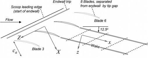
The experimental configuration is based on the work of Muthanna and Devenport (Muthanna and Devenport, 2004), Wang and Devenport (Wang and Devenport, 2004), and Devenport et al. (Devenport et al., 2004) on the linear cascade experiments installed in the Virginia Tech Low Speed Cascade Wind Tunnel. This cascade has been chosen as it is producing a large-scale tip flow with good experimental data for the study of tip-leakage flow as the one encountered inside a turbofan. It corresponds to an eight-blade linear compressor cascade with adjustable tip gap. The blade shape is a 4%-thick modified circular-arc section. The flow downstream of the cascade is guided by two parallel walls on each side of the blades separated by L+h=254mm, with L the span and h the tip-gap size. The chord c is 254 mm and the blades are mounted with a stagger angle of 56.9°, yielding an axial chord ca of 139 mm. In the present study, only one gap size is considered (4.0 mm, or 2.9% ca). The inlet angle is 65.1°, hence the blades see a flow with angle of attack of 8.2°, providing a strongly loaded cascade and hence a strong tip-leakage flow. Given the pitch between blades p=235mm, the solidity for this compressor cascade is σ=p/c=1.08. The Reynolds number based on the chord is 3.88×10⁵ and the Mach number is 0.07. The set-up is shown in Figure 1. Both the Reynolds and the Mach numbers are much lower in this present study compared with the previous study on the isolated airfoil (Koch et al., 2020) (9.6×10⁵ and 0.2 respectively).
Figure 1.
Numerical configuration
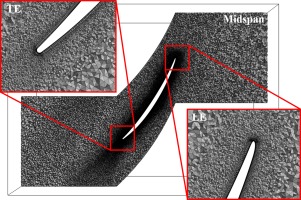
The computations are performed using the compressible LES solver AVBP v7.1 (Schönfeld and Rudgyard, 1999). The numerical scheme for this computation is the explicit Two-step Taylor Galerkin 4A (TTG4A) scheme, which is third order in space and fourth order in time. The time integration is explicit, so the time step is fixed at 2.0×10⁻⁸s in order to ensure a maximum CFL of 0.7. In order to have the proper turbulence decay toward the walls, the sub-grid scale model used is the Wall-Adapting Local Eddy-viscosity model (WALE). The computational domain corresponds to one flow passage of the experimental configuration, which is … The tip-gap size is 4.0 mm (2.9% ca). Translational periodicity is used on both sides of the domain to reproduce the adjacent blade influence, as shown in Figure 2. Navier-Stokes characteristic non-reflective boundary conditions are used at the inlet and the outlet, combined with sponge layers to avoid spurious reflections (Odier et al., 2019). The endwall is stationary. The unstructured mesh is a hybrid one of 120×106 cells with 15 prismatic layers on the airfoil surface and on the lower plate, and tetrahedra elsewhere. It is refined around the airfoil, in the wake, and close to the tip in order to capture the tip-leakage vortical structures. The leading and trailing edges are also refined with the same meshing strategy as the one used by Pérez Arroyo et al. on the LES of the NASA Source Diagnostic Test turbofan (Pérez Arroyo et al., 2019). The wall resolution in wall units is within the range x+<40, y+<3, and z+<40 on the whole airfoil and the lower plate close to the tip. The number of points in the tip gap is around 40 (30 prismatic layers and 10 tetrahedra), with a tetrahedral mesh size of 1 mm around the airfoil and in the TLV region, and 0.3 mm in the tip-gap region. The airfoil and the endwall are modeled as adiabatic walls with zero velocity whereas the top wall (equivalent to the hub in a rotating machinery) is modeled as an adiabatic wall with zero normal velocity (slip wall). The mesh is shown in Figure 3 with zooms on the leading edge (LE) and the trailing edge (TE).
Figure 2.
Numerical domain used for the LES.
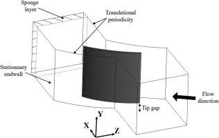
Figure 3.
Visualization of the mesh used for the LES - Plane at midspan.
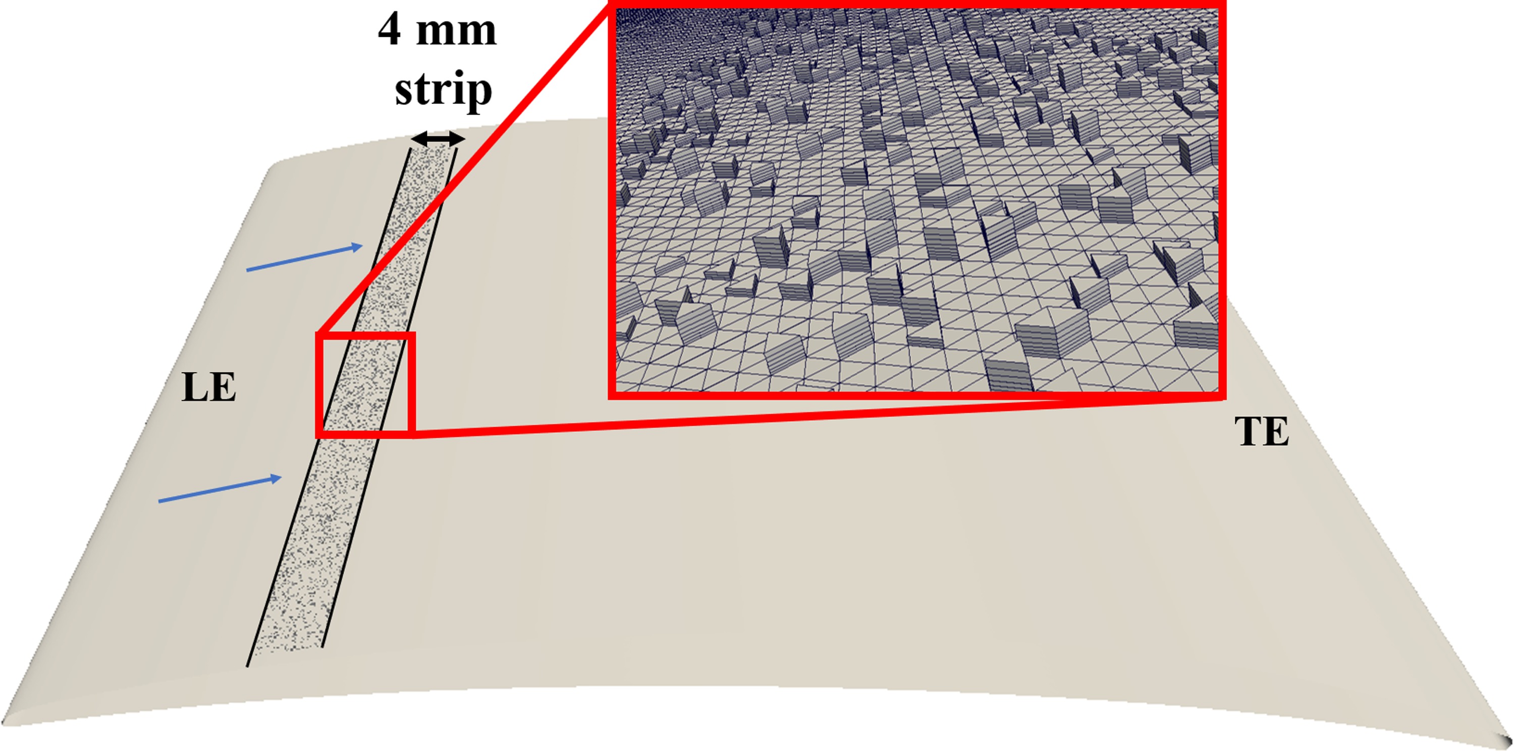
A second configuration is considered as the tripped case. The exact same mesh is used and several prismatic cells are removed randomly from the mesh on a 4 mm (2.0% ca) wide strip on the airfoil suction side at X/ca=0.1. Around 10% of the prismatic cells on the strip are removed. The prismatic height removed is from 3 to 8 cells, also chosen randomly. A total of 21 204 prismatic cells have been removed. This produces a random trip on the suction side, providing a complete random turbulence downstream of the strip. The trip is shown in Figure 4. This method is based on the work of Zhu et al. (Zhu et al., 2018).
Figure 4.
Visualization of the trip with the removed prismatic cells.

The untripped LES has been initialized with a RANS simulation on the same mesh with the solver ANSYS CFX v17. For that calculation, the turbulence model is k−ω SST and both advection and turbulence model equations are resolved with second order schemes. The tripped LES has been initialized with the untripped LES. The data have been obtained from the two LES for a period of about 30 ms (5 flow-through times based on axial chord ca), after the convergence of the computations had been reached. The computations have been achieved on the supercomputer Niagara from Compute Canada, managed by SciNet. A total of 40 nodes, each with 40 Intel Skylake cores at 2.4 GHz have been used for each computation, for a total time of 360 h per computation.
Results and discussion
Pressure coefficient
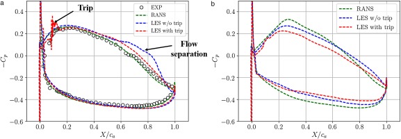
The pressure coefficient Cp defined as (p−p∞)/(0.5ρ∞U∞2) is shown at midspan and at 0.1ca from the tip edge in Figure 5a and 5b respectively. The reference values used for the computations are p∞=101,160Pa, ρ∞=1.225kg.m−3, and U∞=25.2m.s−1. The Cp distribution is compared with experiments. The LES without trip shows relative good agreements with experiments at midspan but the Cp distribution near the trailing edge shows a hump between X/ca=0.6 and X/ca=0.9, which is caused by the suction side boundary layer that separates. The boundary layer then reattaches to the airfoil suction side just before the trailing edge. The multiple peaks on the Cp distribution of the tripped case around X/ca=0.1 highlight the influence of the trip, which generates random fluctuations to trigger turbulent transition. It forces the suction side boundary layer to transition from laminar to turbulent, avoiding a flow separation at the trailing edge. This Cp distribution shows better agreements with experiments. Near the tip edge, the pressure loading is slightly reduced with the trip, which could influence the TLV since it is driven by the pressure difference at the tip. The RANS results at midspan are initially closer to experimental results since the flow is fully turbulent from the leading edge, but do not show the slight flow separation at midchord and underestimate the aft loading. Near the gap, the aerodynamic loading is found more important from RANS results compared with LES results.
Figure 5.
Pressure coefficient distribution - (a): midspan and (b): 0.1ca from the tip edge.
Flow topology
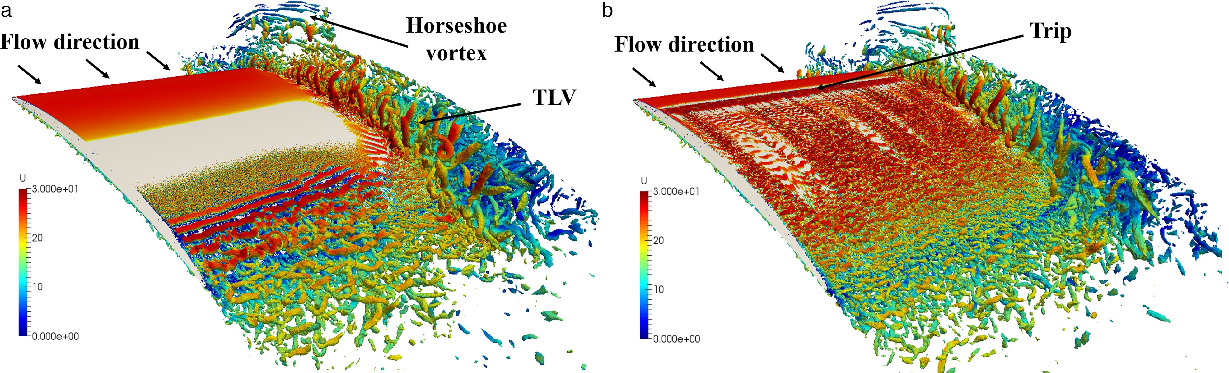
In Figure 6, an isosurface of Q-criterion (106s−2), the second invariant of the velocity gradient tensor, from the instantaneous field colored by the mean velocity magnitude is shown, from the untripped and the tripped cases in Figure 6a and 6b respectively. The Q-criterion allows visualizing the vortical structures of the flow. On the one hand, without the trip, the laminar flow on the suction side separates around midchord. Then, the boundary layer becomes turbulent and reattaches just upstream of the trailing edge. On the other hand, the Q-criterion isosurface of the tripped case in Figure 6b exhibits strong turbulent structures developing from the trip, allowing the boundary layer to resist to the adverse pressure gradient building up after 20% chord. The TLV trajectory seems to differ with the trip: the TLV is located further from the airfoil as it is convected downstream. Near the trailing edge, the large vortical structures that exit the gap interact with the external flow and the wake.
Figure 6.
Q-criterion isosurface colored by mean velocity magnitude - (a): w/o trip and (b): with trip.

RMS velocity fields
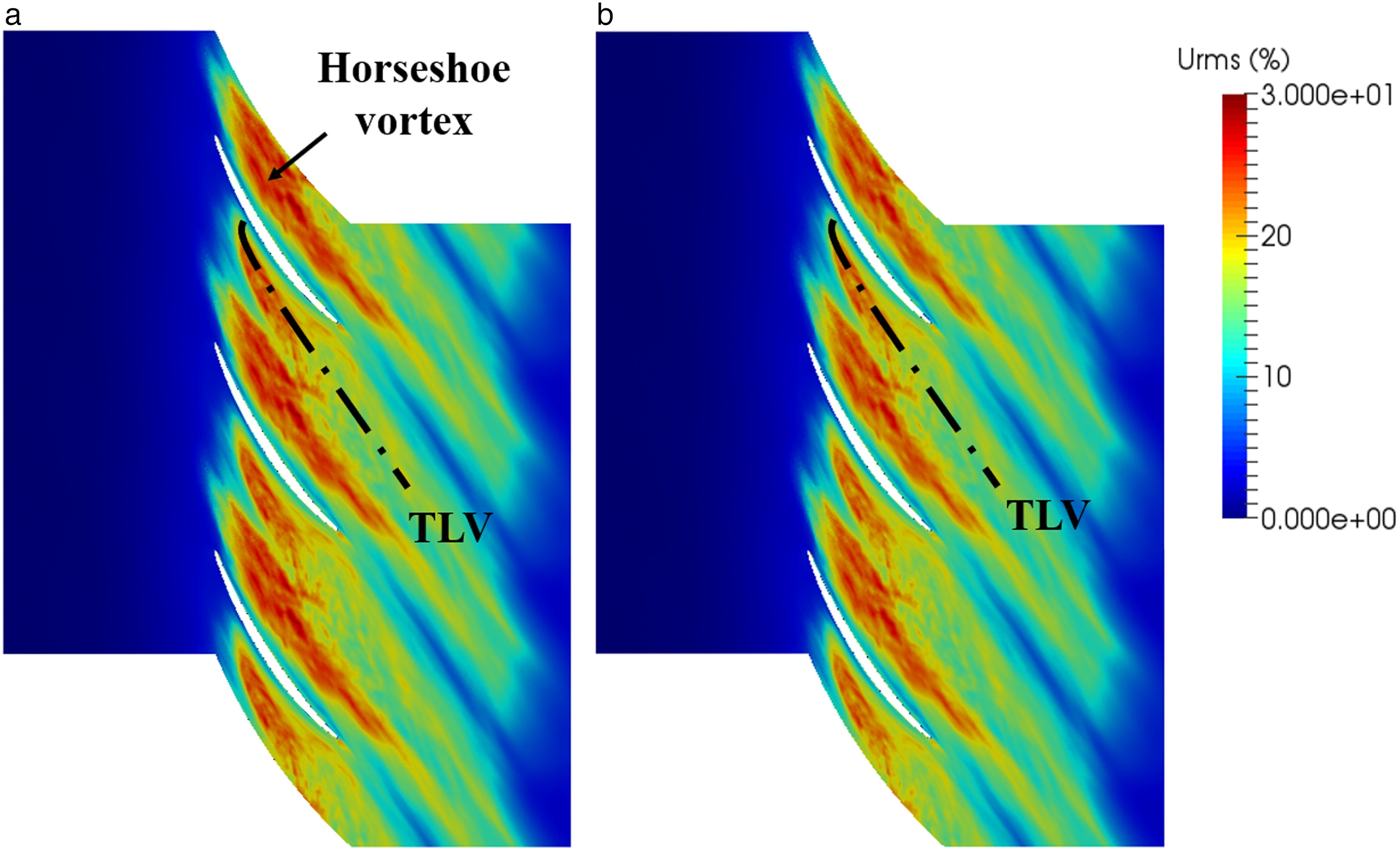
Root-mean square (RMS) velocity magnitude normalized with the inflow velocity in a plane at midspan is shown in Figure 7a and 7b, from the untripped and the tripped cases respectively. The trip reduces the trailing-edge flow separation and induces a thinner wake with lower RMS velocity values downstream of the cascade. The RMS velocity magnitude in a plane at 0.1ca from the tip edge is then shown in Figure 8a and 8b, from the untripped and the tripped cases respectively. The TLV is seen as a high RMS velocity region near the suction side, whose trajectory is indicated as the black doted line. A horseshoe vortex is seen in the middle of the blade passage, also shown in Figure 6. The RMS velocity values in the TLV region are slightly higher with the untripped case.
Figure 7.
Normalized RMS velocity magnitude at midspan - (a): w/o trip and (b): with trip.
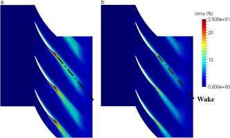
Figure 8.
Normalized RMS velocity magnitude at 0.1ca from the tip edge - (a): w/o trip and (b): with trip.

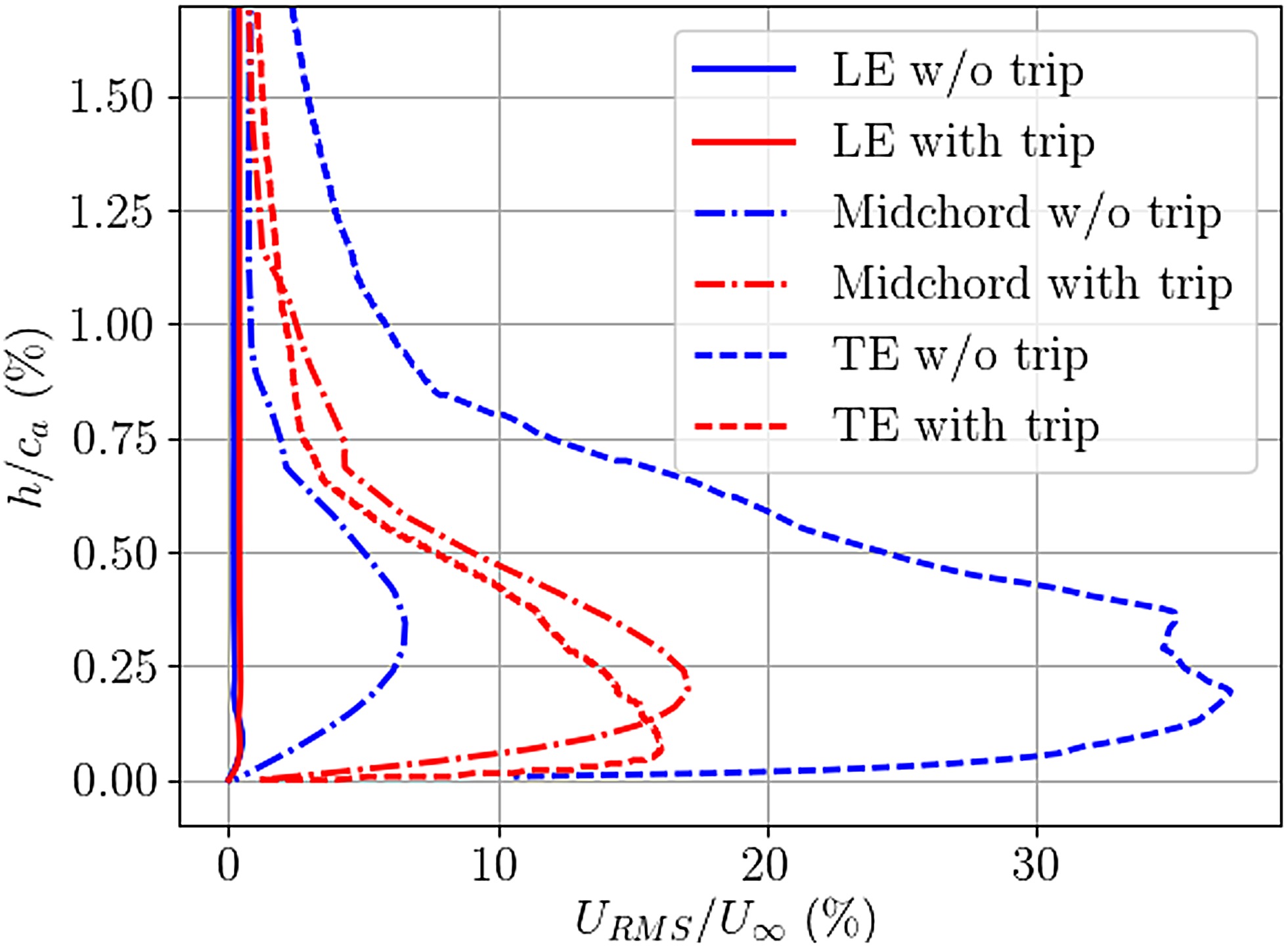
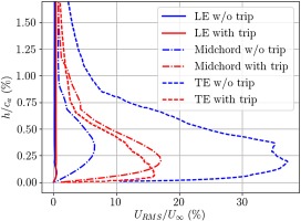
RMS velocity profiles at midspan made at different chordwise position are shown in Figure 9. The RMS values are normalized with the inlet velocity magnitude and plotted as a function of h/ca with h the normal distance from the wall. Three chordwise positions are considered: leading edge (LE), just before the trip (X/ca=0.02); midchord, after the trip (X/ca=0.5); and trailing edge (TE) where the flow separates (X/ca=0.8). Before the trip, the RMS values are identical between both cases, and fairly close to zero. At midchord, the RMS velocity profile from the case with trip shows a much more turbulent flow compared with the case without trip (17% of maximum velocity fluctuation with trip and only 7% without trip). The shape of the tripped case is also more consistent with a turbulent flow (Moreau et al., 2011). At the trailing edge, the maximum RMS value of the case without trip becomes much higher because of the breakdown of the coherent rollers seen in Figure 6. It reaches 37% whereas the tripped case reaches only 16%. The higher RMS values for the untripped case could induce higher far-field noise levels, since the main noise sources related to this configuration are the trailing-edge noise source and the tip-leakage noise source that are both related to surface pressure fluctuations.
Figure 9.
Normalized RMS velocity profiles at midspan for different chordwise positions: LE (X/ca=0.02), midchord (X/ca=0.5) and TE (X/ca=0.8).
Wall-pressure spectra
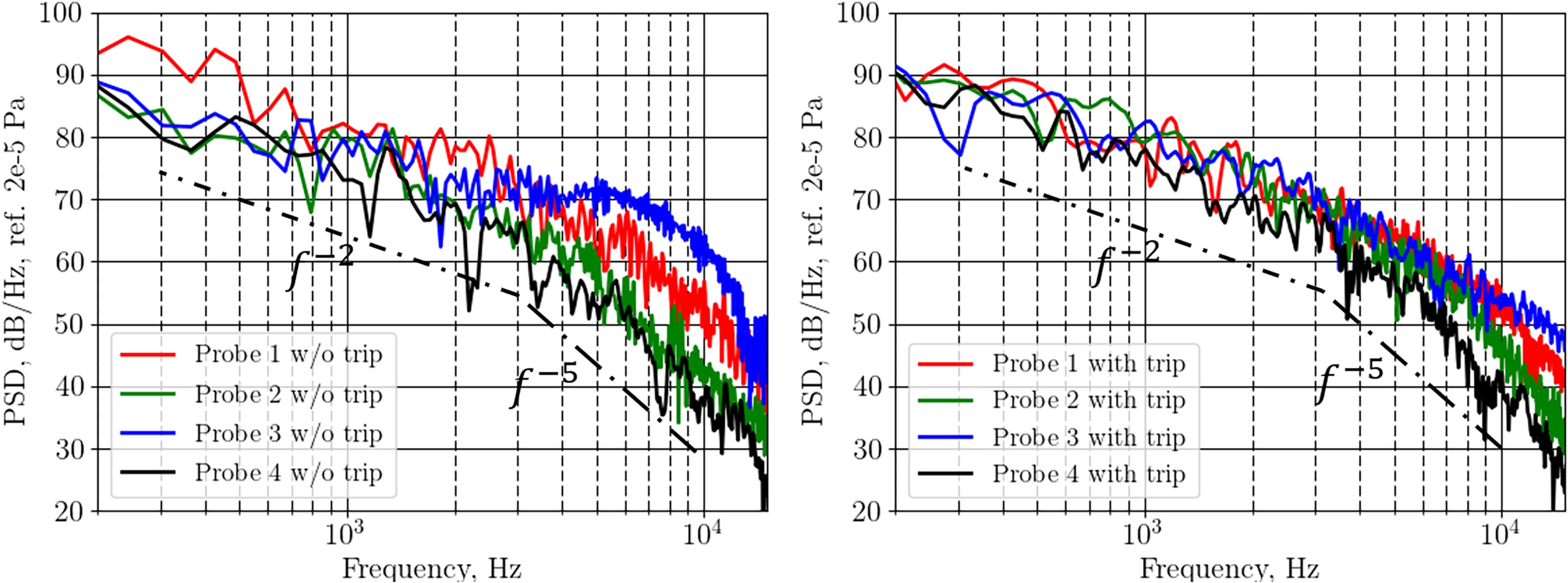
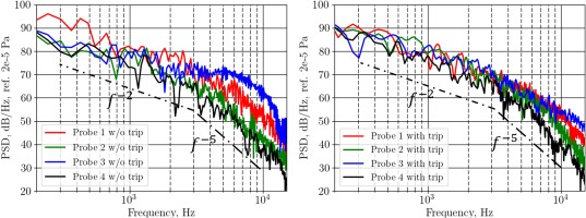
Wall-pressure power spectral density (PSD) on the airfoil suction side at 0.1ca from the tip edge have been recorded at different chordwise positions. Probes 1 to 4 are located respectively at X/ca=0.5, X/ca=0.6, X/ca=0.7 and X/ca=0.8. We focused on this particular zone because it may be one of the major noise source related to tip-leakage flow, according to Koch et al. (Koch et al., 2020). Large vortical structures exit the gap, and the scraping of turbulent structures in the vicinity of edges is an efficient noise mechanism (such as trailing-edge noise). Therefore the wall-pressure PSD for each probe is seen in Figure 10a and 10b for the untripped and the tripped cases respectively. The shape of the PSD spectra for the probes 1, 2 and 4 has a typical slope and shows a decrease of frequencies as f−2 at low frequencies, and as f−5 at high frequencies (Moreau et al., 2011). On both cases, one can see the PSD decreasing from probe 1 to 2, and then a major increase is seen in probe 3, at X/ca=0.7 starting from 2 kHz to 10 kHz. Moreover, the probe 3 exhibits a much higher hump for the untripped case compared with the tripped case, meaning that the noise signature could be influenced by the trip. Finally, probe 4 shows a strong decrease in the wall-pressure PSD after the tip-separation vortex has exited the gap.
Figure 10.
Wall-pressure power spectral density on the suction side at 0.1ca from the tip edge for various chordwise positions - (a): w/o trip and (b): with trip.
Trajectories of the wake and the TLV center
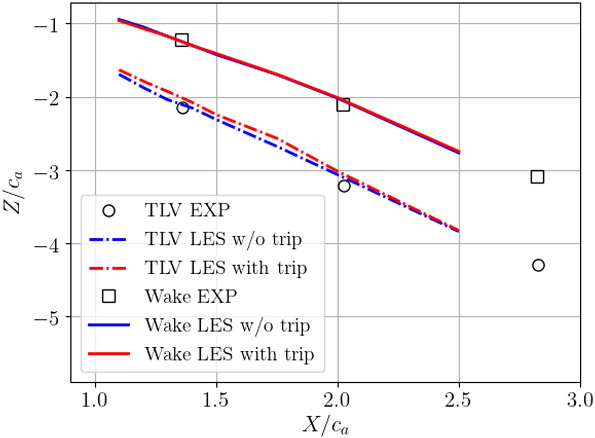
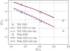
The trajectories of the blade wake and the core of the TLV downstream of the cascade is show in Figure 11. The data from both computations are compared with experimental results of Muthanna et al. (Muthanna and Devenport, 2004). The center of the blade wake is taken as the point of maximum axial velocity deficit at midspan, whereas the center of the TLV is taken as the point of maximum axial vorticity near the endwall. The wake trajectories from both numerical cases are almost identical and aligned with experimental wake trajectory. The TLV trajectories from the untripped and the tripped cases show also very good agreement with experiments. The tripped case trajectory is slightly further from the airfoil suction side near the trailing edge as shown previously, but the two trajectories merge when the TLV reaches the end of the domain.
Figure 11.
Comparison of the trajectories of the blade wake and the core of the TLV downstream of the cascade.
Velocity and vorticity fields downstream of the cascade
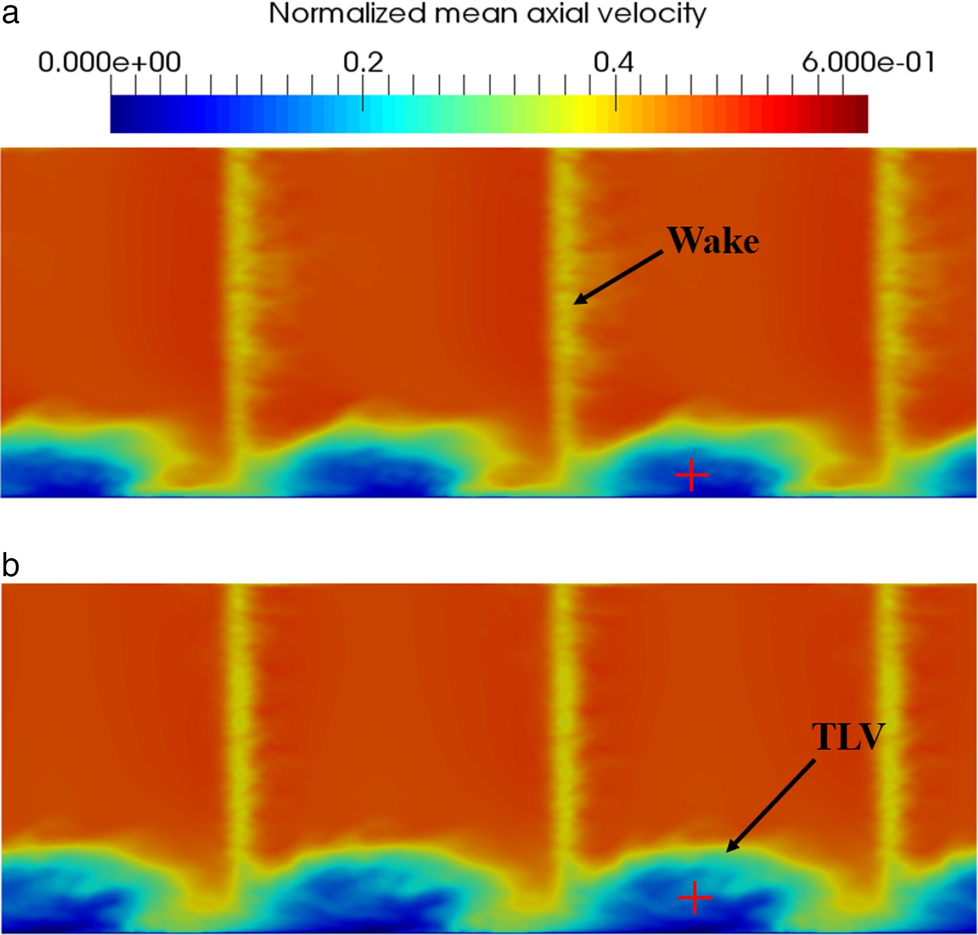
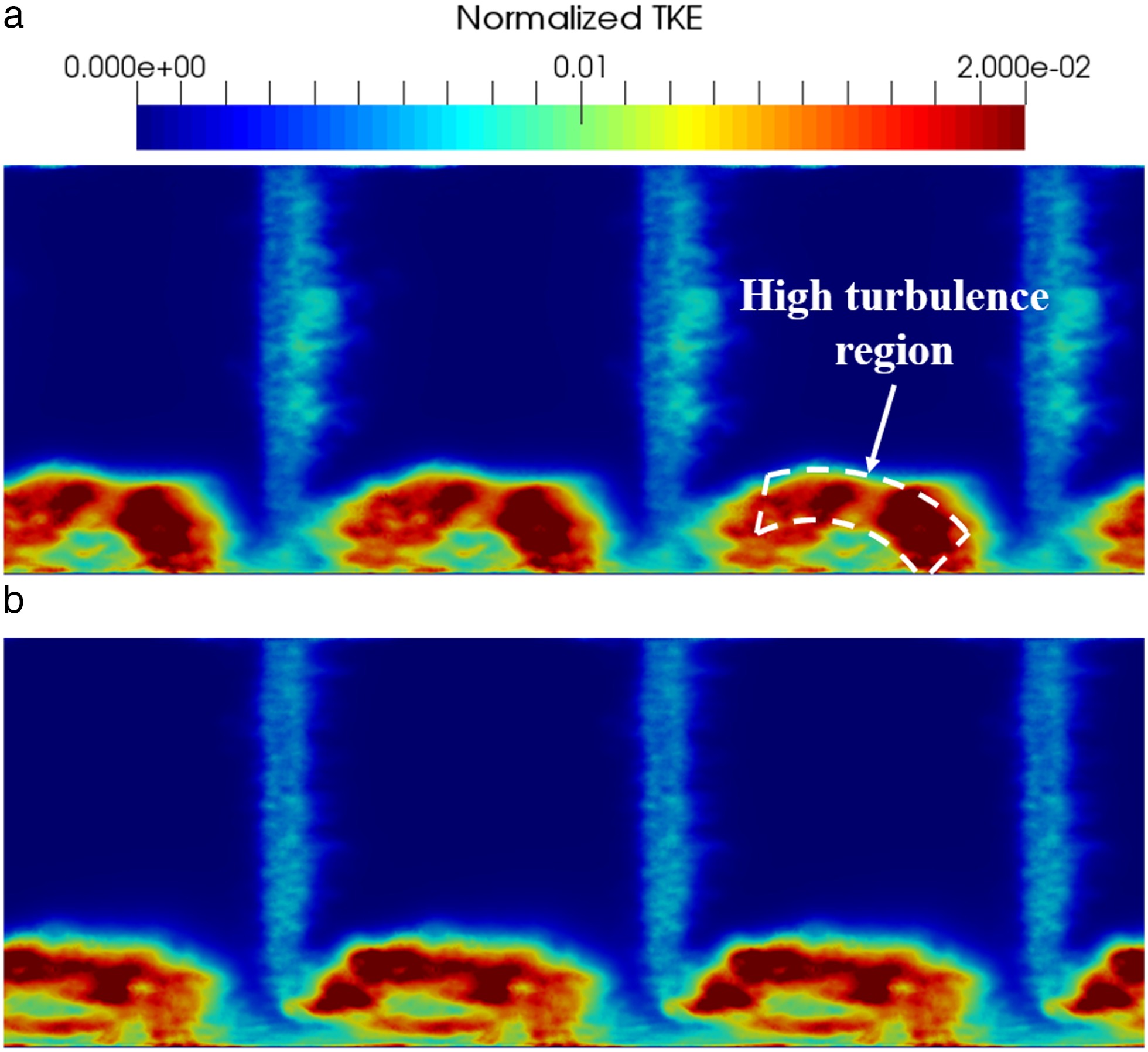
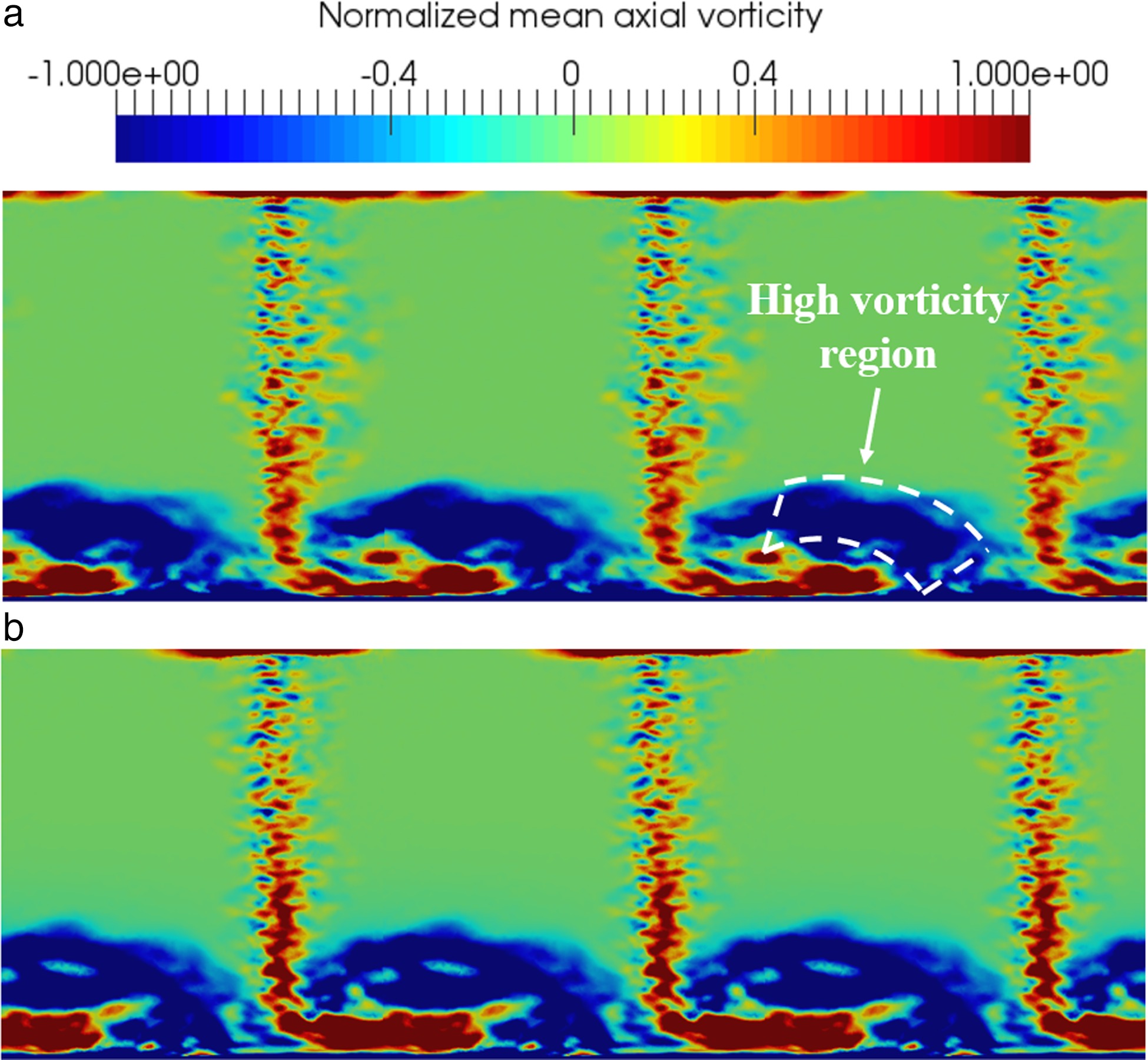
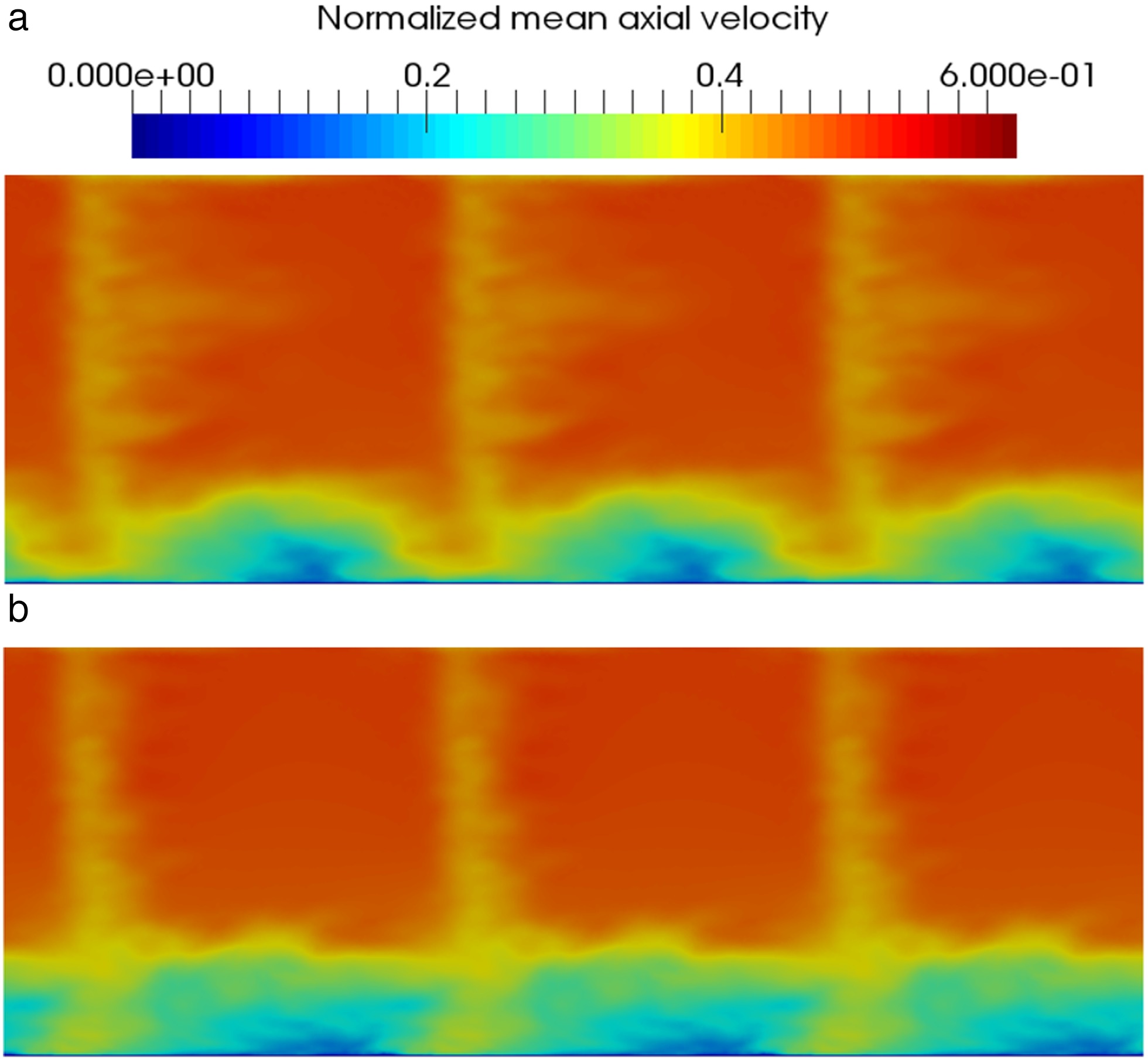
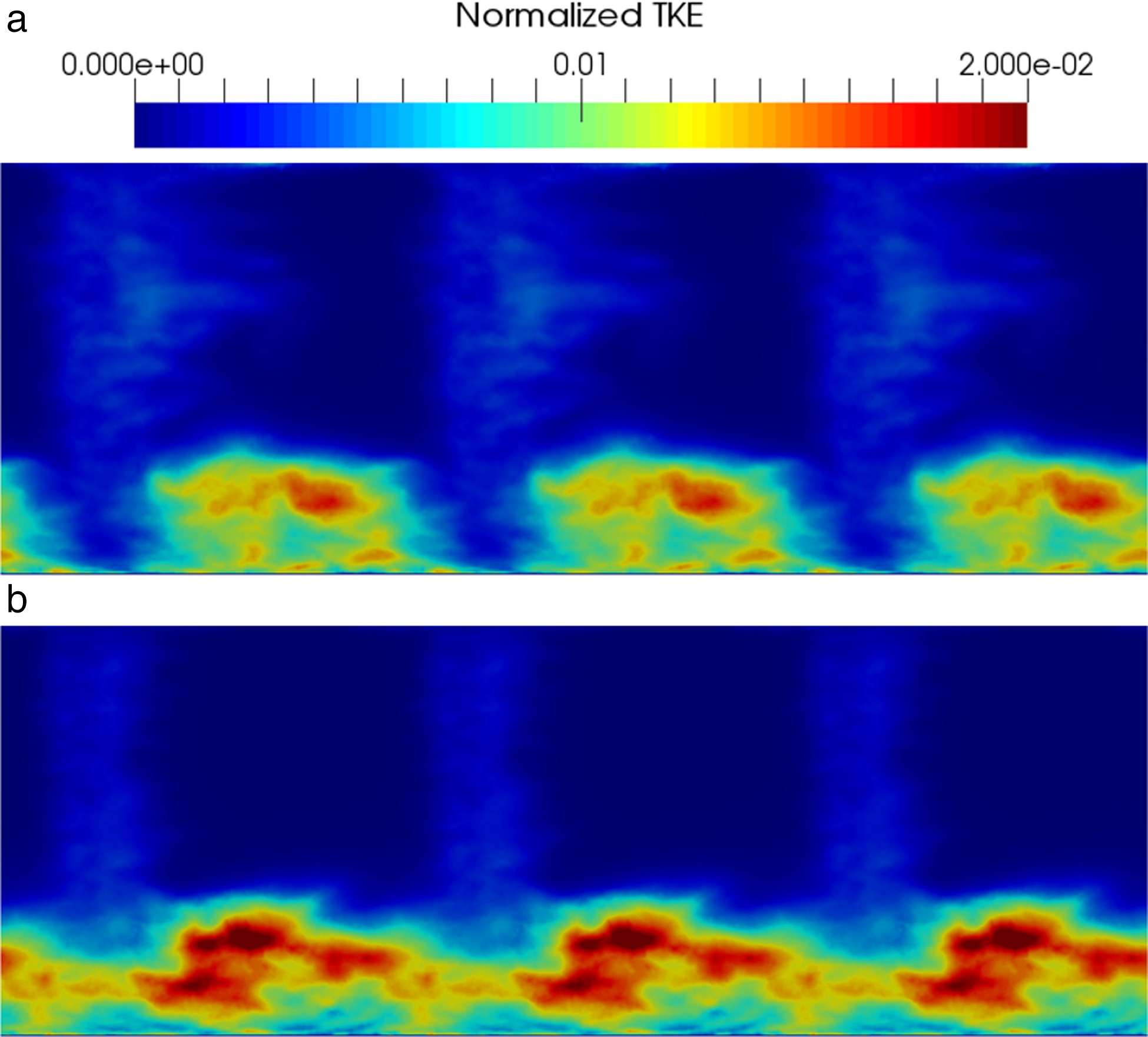
The flow structure downstream of the cascade is analyzed through two cross-sectional planes (Y, Z) at X/ca=1.37 and X/ca=2.06 called plane 1 and plane 2 respectively. These planes correspond to the positions of the measurement stations used by Muthanna et al. (Muthanna and Devenport, 2004) and Wang et al. (Wang and Devenport, 2004). You et al. (You et al., 2007) also used these same planes in their LES analysis. The velocity components along X, Y, and Z are labeled U, V, and W respectively. Mean axial velocity (U) normalized by the inflow velocity at plane 1 is shown in Figure 12a and 12b for the untripped and tripped cases respectively. The TLV is seen as a large velocity deficit close to the endwall and the red cross represents its center. The tripped case shows thinner wakes and a larger TLV that is lifted up from the endwall compared with the untripped case. Turbulent kinetic energy (TKE) normalized by the square of the inflow velocity at plane 1 is seen in Figure 14. Maximum TKE values are localized along an ellipse that borders the top of the TLV, as shown with the white doted lines. This turbulence is created by the strong axial velocity gradients in the outer part of the TLV. Mean axial vorticity defined by Ωx=∂W/∂Y−∂V/∂Z normalized by the inflow velocity and the axial chord (Ωxca/U∞) at plane 1 is seen in Figure 16. Maximum vorticity values also reach the same region of the TLV. Muthanna et al. made the exact same observations during their experiments. The structure of the TLV remains the same between both cases but the tripped one still exhibits a slightly stronger and wider vortex. Especially, the jet flow passing from the pressure side to the suction side shows higher vorticity values in Figure 16b.
Figure 12.
Normalized mean axial velocity at X/ca=1.37 - (a): w/o trip and (b): with trip.

Figure 14.
Normalized turbulent kinetic energy at X/ca=1.37 - (a): w/o trip and (b): with trip.
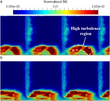
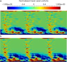
Figure 16.
Normalized mean axial velocity at X/ca=1.37 - (a): w/o trip and (b): with trip.
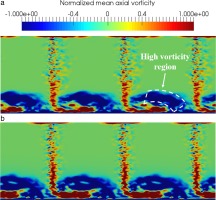
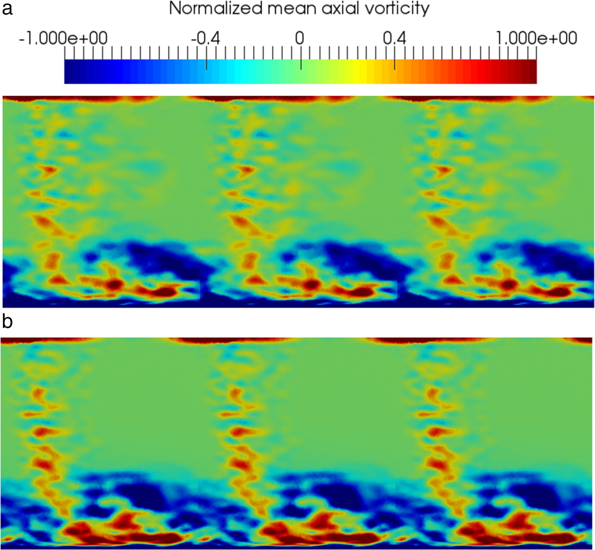
Mean axial velocity and TKE normalized by inflow velocity and mean axial vorticity normalized by inflow velocity and axial chord at plane 2 are shown in Figures 13a–15a–17a and 13b–15b–17b for the untripped and tripped cases respectively. The differences observed between the untripped and tripped cases at plane 1 remain the same at plane 2. The growth of the airfoil wake and the TLV is clearly visible. The later tends to be distorted by its interaction with the endwall. Once again, the same observations have been made by Muthanna et al. and You et al. Nevertheless, the TLV of the tripped case diffuses in a slower manner than the untripped case. TKE and vorticity values are higher at plane 2 compared with the untripped case. The maximum TKE and vorticity region is located at the top and left-hand side of the TLV for the tripped case whereas it is at the right-hand side for the untripped one and experiments.
Figure 13.
Normalized mean axial velocity at X/ca=2.06 - (a): w/o trip and (b): with trip.
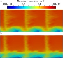
Figure 15.
Normalized turbulent kinetic energy at X/ca=2.06 - (a): w/o trip and (b): with trip.
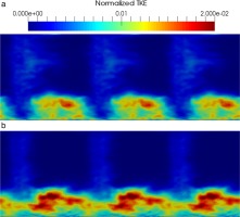
Figure 17.
Normalized mean axial vorticity at X/ca=2.06 - (a): w/o trip and (b): with trip.
Conclusions
A first compressible wall-resolved LES of a linear compressor cascade with tip gap has been achieved in order to investigate the aerodynamic mechanisms responsible for the TLV formation and its behavior as it is convected downstream. As observed by Muthanna et al. and You et al., the TLV grows and distorts due to the endwall. Maximum turbulence levels are located along an ellipse at the top of the TLV and coincides with maximum vorticity region. This study has also highlighted the influence of the suction side boundary layer development on the TLV. A tripped boundary layer produces a wider and stronger TLV that diffuses slower than an untripped one. The region of high turbulence and vorticity levels is located on the right-hand side of the TLV for the untripped case and experiments, whereas it is located on the left-hand side for the tripped case. The trip also tends to lift up the TLV from the endwall, and move it away from the airfoil suction side. Although the main characteristics of the TLV remain the same between both cases, the trip still influences the development of the TLV near the gap and downstream of the cascade. A deep aeroacoustic investigation will be done in order to correlate these observations with noise emissions from the tip-leakage flow. Since surface noise sources are related to the RMS pressure fluctuations on the airfoil, the presence of the trip might modify the far-field noise signal due to the different flow behavior near the trailing edge between the tripped and the untripped cases. In this future study, the influence of the single flow passage configuration will have to be compared with a multiple blade computation in order to highlight the main differences that could occur, since the single blade configuration can correlate the acoustic signal from one blade to another.