


Introduction
Valley glaciers and small ice caps respond sensitively to climate on a relatively short time-scale (Oerlemans and Fortuin, 1992; Oerlemans, 1994). They can thus serve as indicators of climate change. Recent work has shown that the retreat of many glaciers and ice caps may have been one of the main factors that have led to a global sea-level rise during the past century (Meier, 1984; Warrick and Oerlemans, 1990; Wigley and Raper, 1993). In situ measurement of glacier mass balance is obviously the best way to infer climatic change from glaciers. However, it is labour-intensive. Although such monitoring has been done on some glaciers, the records available are generally short (less than 30 years). Records of glacier length, on the other hand, extend over longer periods. Some of them date back to AD 1600. Historical variations in glacier length can provide us with information about climatic variability in the past. By understanding the relation between glaciers and climate in the past one can predict the future behaviour of glaciers under various climate scenarios.
Several attempts have been made to simulate historic glacier variations over the past few centuries using a numerical ice-flow model (Kruss, 1984; Oerlemans, 1986; Huybrechts and others, 1989; Stroeven and others, 1989; Greuell, 1992). In these studies, the evolution of a glacier was simulated with a mass-balance history reconstructed on the basis of climatic records and/or other proxy data. One of the problems in simulating a glacier variation is the state of a glacier with respect to the corresponding climate. In previous studies, the flow model was calibrated in such a way that the difference between the observed and the simulated present length of the glacier was minimized under a steady-state condition. However, it is not known whether a glacier state provided by up-to-date glacier maps is actually in balance with the present climate. Thus, the way in which the performance of an ice-flow model is judged in previous studies is obviously inappropriate.
In this study a different approach, namely dynamic calibration as proposed by Oerlemans (1997), is used in a one-dimensional ice-flow model to simulate the front variation of the Pasterze glacier. The Pasterze is the largest glacier in the Austrian Alps. It was chosen for this study for several reasons: it is relatively large and has a regular shape; data on the front variation and some data on the mass balance are available; and, as a result of data collected during an extensive glacio-meteorological experiment (PASTEX; Greuell and others, 1995) in the summer of 1994, we have been able to learn more about the glacier behaviour.
In the following sections, we first define the glacier geometry and a reference mass-balance profile. Then a dynamic calibration is performed to yield the required mass-balance changes that correspond to the observed front variations of the Pasterze. During the calibration procedure the flow model is adjusted. The deduced mass-balance changes are then checked against existing climate records, particularly air temperature and precipitation, to determine the mass-balance sensitivity. The next step is to verify the derived sensitivity in order to use it to model the future behaviour of the Pasterze. We do this by first reconstructing
Table. 1 Topography of the Pasterze glacier


Fig. 1. Map of the Pasterze, showing the glacier stand in 1985 and the maximum stand around 1851. Thick lines are the flowlines with grid points used in the model. Five sites of the PASTEX experiment are also shown.
a mass-balance history on the basis of the temperature record using the derived sensitivity, then using the reconstructed balance history as a forcing to simulate the observed front record. Some sensitivity experiments will also be presented. Finally, projections of the future behaviour of the Pasterze are attempted under various climate scenarios.
The Pasterze Glacier
The Pasterze (47∘06’ N, 12∘ 43’ E) is the longest glacier in the Austrian Alps. A general picture of the topography can be obtained from Table 1 and Figure 1. In 1969, the glacier was approximately 9.2 km long and had a surface area of 19.8 km2 (Rott, 1993). Its general exposure is southeast. At present, the Pasterze has two tributaries: Teufelskampkees and Glocknerkees. The other two tributaries, Hofmannskees and Wasserfallwinkel, contributed ice to the mainstream in the past.
Little is known about the length variation of the Pasterze before 1880. Annual length measurements were initiated in 1880 (Bachmann, 1978) and have continued up to the present (Fig. 2). End moraines indicate the glacier stand around 1635 (Lang and Lieb, 1993), although little is known about the state of the glacier at that time. Historical documents and other published observations reveal that other Alpine glaciers have undergone similar periods of advance and retreat over the past 400 years. After a glacier advance in the early 17th century, the Pasterze remained in a fairly stable position, with only small variations over the next 250 years (Rott, 1993). Like most east Alpine glaciers, as seen in Figure 2, it reached its maximum around 1851. Since that time it has receded continuously, although the rate of the retreat was somewhat low (≈2 m year–1) between 1910 and 1930. In fact, glacier retreat seems to have been a worldwide phenomenon for the past century (Porter, 1986; Oerlemans, 1994). The recession of the Pasterze is very probably attributable, at least in part, to long-term climatic conditions that are conducive to negative mass balance.
Observations made on the glacier surface (Tintor and Wakonigg, 199!; Wakonigg, 1993; Bayr and olhers, 1994) have shown that the terminus of the glacier has retreated each year since the winter of heavy snow in 1965–66, the total recession being nearly 400 m. Studies based on Landsat thematic mapper data (Hall and others, 1992; Bayr and others, 1994) have also suggested that between 1984 and 1990 the terminus of the Pasterze receded at an average speed of approximately 15 m year–1. Data for 10 year mass-balance measurements are available as a result of the Tauern power station project (TKW; Tintor, 1991). The measurements

Fig. 2. Historic length variations of the Pasterze glacier.
indicate that the mean equilibrium-line altitude (ELA) of the Pasterze during 1979–89 was 2880 m a.s.l.
ICE-Flow Model
The one-dimensional ice-flow model is based largely on the one used in Oerlemans (1986) and Greuell (1992). The major improvement is in the dynamic calibration (this will be discussed in detail in the next section).
The ice flow is calculated along the central flowline (x axis). Seven flowlines are modelled due to the complexity of the Pasterze geometry (Fig. 1). Three of them are on the main ice body: the mainstream (along Pasterzen Kees), the left stream (on the orographically left side of Oberster Pasterzeboden) and the right stream (on the orographically right side of Oberster Pasterzeboden), as indicated in Figure 1. The remaining flowlines are on the tributaries. The grid spacing is 200 m. Geometry digitizing for the Pasterze and the tributaries is based on the topographic map of Gross-glocknergruppe (1:25000; Der Deutsche Alpenverein und Der Oesterreichische Alpenverein 1992) and is done in such a way that the area–elevation distribution is preserved.
Parameterization of the cross-section profile includes implicitly the three-dimensional geometry at each grid point. The cross-section profile can be reasonably well represented by a trapezoidal shape. The profile is determined by the elevation of the glacier bed (h b), the width of the bed (W b) and the angle of the slope on the left (α L) and right (α R) side of the valley (Fig. 3). Since few data are available on the ice thickness (H) of the Pasterze, the thickness is initially estimated from a constant driving stress (assuming

Fig. 3. Schematic illustration of the cross-section geometry.
τ d = 1.5 bar; i.e. slope x ice thickness = 17 m). The bed profiles are then generated from the ice thickness and the valley geometry. Thus the cross-sectional area (S) can be expressed as:

By solving a continuity equation in S (taking a constant ice density), one can calculate the changes that have occurred in ice volume:

where U is the mean velocity of the cross-section, B is the mass balance, W s is the width of the glacier surface and x is the downstream distance along the flowline (x = 0 at the head). The total ice velocity U is the sum of the internal

Fig. 4. Mean profile of the 10 year mass-balance measurements (1979–89) on the Pasterze glacier and the data fit used in the calculation as the reference profile (Bred). The filled dot is an estimated value (see text).
deformation velocity (U d) and the sliding velocity (U s). U d and U s are calculated according to Paterson (1994). Flow parameters f 1 and f 2 are taken on the basis of empirical studies done by Budd and others (1979). Some adjustments were made (i.e. f 1, f 2 are one-sixth of the original values) to obtain realistic output (f 1 = 3.17 x 10⁻²⁵ m6 s–1 N–3, f 2 = 8.38 x 10⁻¹⁷ m5 –1 N–2). In the calculation the contribution of basal water to sliding is not explicitly taken into account; instead a bulk effect is included in the sliding parameter f 2.
The ice influx from the sub-streams and the tributaries is considered in the calculation. The ice flow along all the flow-lines is calculated simultaneously during the time integration. The ice flux at the last two grid points of the substream or tributaries is calculated at the point where the ice streams meet. The flux is then converted to ice thickness ΔH. With every time step Δt, ΔH is evenly divided and added to the nearest three grid points in the mainstream.
Dynamic Calibration
The procedure for the dynamic calibration follows Oerlemans (1997). It is assumed that at any time the mass-balance profile B(h s) can be described as:
where B ref is the reference mass-balance profile which is independent of time t, and ΔB(t) is a perturbation in mass balance which is independent of elevation h s.
The calibration proceeds as follows: (1) existing mass-balance observations are compiled to obtain a reference mass-balance profile B ref; (2) perturbations in mass balance ΔB are then imposed upon the profile, independent of elevation, to determine the mass-balance changes that occurred in the past. This is done, by trial and error, in such a way that a best approximation between the simulated and the observed glacier length variation is achieved; (3) snapshots of the model simulation are compared with available data, and the model geometry is adjusted if there is a significant discrepancy.
To obtain a reference balance profile we use a mean of the mass-balance observations made for the work of TKW during 1979–89 (Tintor, 1991). The data of TKW were unfortunately all collected in the ablation area (below

Fig. 5. Simulation of the glacier front variation achieved by using the dynamic calibration approach.
2800 m a.s.l.). During the PASTEX measurements, the observed ablation rates in the accumulation area were 0.021 m w.e. d–1 at about 3200 m a.s.l, and 0.032 m w.e. d–1 at about 3000 m.a.s.l. (Greuell and others, 1995). Taking into account the observed ablation period of 87–134 d year–1 on the Pasterze (1980–84; Tintor, 1991) and the mean annual precipitation rate of 2.58 m year–1 (1891–1930 at the Sonn-blick station; Tollner, 1951), we estimated a mass balance of 0.5 m w.e. year–1 at 3000 m a.s.l. A fit to the mean profile of the TKW data and the estimated mass balance (Fig. 4) is taken as the reference profile B ref. Since no precipitation data are available on the glacier, the data collected at the Sonnblick station (3106 m a.s.l.), 15 km east of the Pasterze glacier, are considered to be the best choice. By definition (Equation (3)) the mean ΔB for the reference period 1979–89 is thus zero.
Using B ref, we determine ΔB for the period 1600–1990 according to the above-mentioned steps (Fig. 5). At first a ΔB (+ 1.33 m w.e. year–1) is taken in such a way that the glacier stand in 1635 represents a steady state since little is known about the glacier state at that time. With a slight increase in ΔB (+ 1.43 m w.e. year–1) in the period 1828–46 and thereafter a balance condition similar to that of the reference period (ΔB = + 0.1 m w.e. year–1) for the next 20 years, the model mimics correctly the timing and stand of the 1851 maximum, as well as the retreat thereafter. The glacier regression since 1866 is very well reproduced, as shown in Figure 5.
During the calibration, the bed geometry is adjusted slightly to fit the observed surface (the topographic map). After the calibration the rms difference between the modelled and the observed surface elevation for 1985 is found to be 15 m. Repeating the calibration procedure could further reduce the discrepancy, but it was not considered meaningful in view of other uncertainties in the model.
Figure 6 shows two snapshots (1851 and 1985) for the mainstream of the Pasterze taken from the model simulation. The calculated ice surface of 1985 matches well with the measured surface. The maximum discrepancy in the surface elevation over the entire profile is 43 m; it is found below the icefall (x = 5.0 km; Fig. 6). The front position of 1851 agrees with the observed maximum stand. The calculated total ice velocity U typically ranges from 10 to 35 m year–1, with a maximum value of 136 m year–1 in the icefall. These model results are compatible with measurements on the Pasterze: the annual mean surface velocity,

Fig. 6. Simulated glacier surface of the mainstream for 1985 and 1851, compared with the measured ice surface in 1985 and with the maximum glacier stand in 1851.
measured in 1970–90 at 2200–2470 m a.s.l., was found to be typically 10–50 m (Wakonigg, 1993). The seismic refraction measurements, carried out by Bittmann and others (1973) in 1970 on the upper part of the glacier (Oberster Pasterzeboden), indicate that the maximum ice thickness exceeded 180 m. Bittmann and others (1973) estimated a typical ice thickness of 90–160 m and an ice volume of 1.22 km3 in that part of the glacier. These values are in broad agreement with the model results of 1970: a typical ice thickness of 80–180 m and an ice volume of 1.28 km3 in roughly the same area.
Figure 7 presents snapshots of 1985 for the sub-stream and tributaries. The simulated ice surface compares well with the observations except in the lower reaches of the two disconnected tributaries (Fig. 7e and f). This is probably because that the actual mass-balance profiles of these two tributaries are somewhat different from the reference balance profile used in the model. Different exposures and different surface conditions would influence the surface energy balance, and thus affect the mass-balance profile. However, the calculated surface areas of the Pasterze glacier including the tributaries for the years 1850 (26 km2), 1925 (25 km2) and 1969 (24 km2) are similar to the values suggested by Rott (1993) for the same periods (28 km2 in 1850; 26 km2 in 1925; 23 km2 in 1969).
Determination Of The Mass-Balance Sensitivity
In this section we will investigate whether there is a meaningful correlation between the deduced mass-balance changes and available climate records. If there is, then we can derive a mass-balance sensitivity for the Pasterze. The mass-balance sensitivity is defined as ΔB/ΔT: the change in mass balance ΔB due to a change in temperature ΔT.
As a first step, climate records for the last few centuries are compiled for the Pasterze. The annual mean air temperature at the Sonnblick station since 1887 is available and is used for our calculation concerning the Pasterze. Unfortunately there is a gap in the data (obtained from World Climate Disc, Chadwyck-Healey Ltd 1992) for the period 1931–50. Climate records from other stations, therefore, have to be used in order to reconstruct the balance history before 1887 and for the gap period. Records of the annual mean temperature have been collected from three other high-altitude climate stations in the surrounding areas of
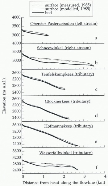
Fig. 7. Calculated ice surface of the sub-streams and tributaries for 1985, compared with the measured surface elevations.
the Pasterze. An impression of the series collected at Säntis (Switzerland), Vent (Austria), Zugspitze (Germany) and Sonnblick is given in Figure 8.
Comparison of the annual mean temperature at Sonn-blick and at other stations indicates that records at Säntis, Vent and Zugspitze are well correlated (R = 0.83–0.90) to the Sonnblick data. The annual mean temperatures for the gap period and for the period 1850–87 are therefore computed from the mean of the Säntis, Vent and Zugspilze data using linear regression equations. Thus, the reconstructed temperature series covers the period 1850–1990. In the reconstructed temperature series ΔT is defined as the temperature difference with respect to the initial temperature (T 0 = –6.45∘C), which is an average value for the period 1850–59. Attempts have also been made to reconstruct the changes in precipitation ΔP, summer temperature ΔT summ (June–August) and melt-season temperature ΔT melt (May–September) for the Pasterze.
The deduced mass-balance changes ΔB are then plotted against the computed ΔP (as well as ΔP, ΔT summ and ΔT melt). As a result, a significant correlation is found between the 5 year mean ΔT and ΔB (R = 0.63, n = 141 years; ΔB/ΔT =–0.859 m w.e. K–1 year–1). A notable

Fig. 8. Temporal variation in the annual mean temperature and the melt season (May–September) temperature at Sonn-blick and three other stations.
correlation between the melt-season temperature change ΔT melt and ΔB is also found, but only for the reference period (1979–89) (R = 0.60, ΔB/ΔT melt = –0.513 m w.e. K–1 year–1. There is no clear dependence of ΔB on ΔP and ΔTsumm . Oerlemans (1993) has suggested a value of –0.473 to –0.632 m w.e. K–1 year–1 for ΔB/ΔT for Alpine glaciers, on the basis of a general study with a mass-balance model. Apparently the sensitivity found here for the Pasterze (–0.859 m w.e. K–1 year–1) is somewhat greater. However, our value is similar to the sensitivity found by W. Greuell (–0.8 m w.e. K–1 year–1; personal communication, 1996) for the Pasterze glacier, as calculated with an energy-balance model using the PASTEX data.
Simulation Of The Front Record Using The Reconstructed Mass Balance
So far we have found a dependence of ΔB on ΔT and have derived a mass-balance sensitivity for the glacier. In this section the derived sensitivity is verified by using the reconstructed mass-balance history as a forcing to simulate the observed front record.
Two types of forcing are considered here (see Table 2). As seen in Figure 9, the forcing period in forcing 1 starts in 1865. As an initial profile, we take the steady-state length corresponding
Table. 2 Forcing used to simulate ih front record, 1865–1990


Fig. 9. Simulation of the historic front record achieved by using various reconstructed series of mass-balance perturbation ΔB(t) as forcing.
to the 1635 position and the maximum length around 1851. The calculated glacier recession since the maximum stand reproduces reasonably well the observed fluctuations of the glacier front. Better results should not be expected since the mass-balance change for Alpine glaciers is not solely a function of the temperature variation. Nevertheless, the model simulation indicates that the flow model used here depicts the ice dynamics on the Pasterze reasonably well, and the derived sensitivity is basically correct. For projecting the future behaviour of the Pasterze, however, the effect of precipitation should be included.
The sensitivity derived from the melt-season temperature change ΔT melt and ΔB is used to rebuild the mass-balance history, which is referred to as forcing 2 (table 2). As demonstrated in Figure 9, the simulation gives a poor result. The modelled glacier length since 1880 is too short and the glacier has retreated too fast compared with the observation. The most obvious explanation is that changes in temperature during the melt season alone cannot account for the changes in mass balance on the Pasterze, even though a correlation exists between the two and this correlation is statistically significant.
Sensitivity Experiments
Theoretically, given a constant mass balance, the glacier length change in time ΔL(t) will eventually approach zero as the glacier reaches steady state. We define the steady state as the glacier state at time t when |ΔL(t)|/L(t) = 0.01%; the length L(t) here is thus called the steady-state length. Figure 10 shows the steady-state length corresponding to the imposed mass-balance perturbation in the upper panel; the state of the glacier (expressed in years away from the defined steady state) is illustrated in the lower panel. Obviously, most of the time the glacier front has been far from the steady-state length. Even if a terminus position is close to the steady-state length, this does not imply that the glacier is close to a steady state.
We also perform some experiments concerning the response time of the Pasterze. We define the length response time τ L as the time required to reach (1–e–1) of the total length change ΔL tot due to a perturbation in mass balance ΔB. The volume response time τ v is the time required to reach (1––1) of the total volume change ΔV tot due to a perturbation in mass balance ΔB. First, a run is made until a

Fig. 10. Steady-state length of the glacier with respect to the imposed mass-balance perturbation and the state of the glacier (expressed in years away from the defined steady state).
steady state is reached (this takes about 500 years, starting with zero ice volume), then an extra anomaly ΔB is imposed, independent of elevation and time. The glacier then adjusts itself towards a new steady state. Results of the experiments are listed in Table 3, together with some values found in the literature. The length response time (70–137 years) is generally longer than the volume response time (34–50 years). This is due to the importance of the geometry factor. The larger the mass-balance perturbation ΔB, the shorter the response time.
The next step is to check whether the deduced mass balance B{t) is stable and justified. Figure 11 shows glacier length variation in experiments in which a sudden additional perturbation in mass balance (±0.5 m w.e. year–1) is imposed in the past. First, a constant perturbation (±0.5) is added in the period 1790–1800 when the model glacier was still under the steady-state condition. Apparently, it takes about 100 years for the perturbation to damp out. Next, the same perturbation in mass balance is imposed in a different period, 1830–40. During this time the model glacier was in a
Table. 3 The length and volume response time of the Pasterze glacier, compared to values found in the literature


Fig. 11. Glacier length variation resulting from a sudden additional perturbation in mass balance (±0.5 m w.e. year–1) in the past.
non-steady state. In this case it takes much longer (>150 years) for the perturbation to damp out. From these experiments one can conclude that the deduced mass-balance curve is indeed justified, since a small alteration in mass balance, even if only imposed in the past, would have led to a large deviation in the length evolution. Moreover, the glacier seems to have a significantly longer memory of its mass-balance history under a non-steady-state condition than under a steady-state condition.
Future Behaviour Of The Pasterze Glacier
Projections of the behaviour of the Pasterze for the next century are made under various climate scenarios. The mass-balance perturbation associated with various scenarios is computed using the derived sensitivity.
Values of ΔT for the period 1990–2100 are taken from the estimated temperature changes under the UN Intergovernmental Panel on Climatic Change (IPCC) scenarios (personal communication from J. R. de Wolde, 1996). De Wolde has calculated annual ΔT for the period 1765–2100 for the grid-box 45-50∘ N (taking ΔT = 0 in 1765), on the basis of a zonally averaged energy-balance climate model (de Wolde and others, 1996). The climate model was calibrated against observations of the present-day seasonal cycle. It was forced by the IPCC radiative forcing scenarios IS92 (including and excluding the aerosol effects). The grid-box ΔT is compared to the ΔT of the Sonnblick series (Fig. 12a). Obviously, the trend in both the Sonnblick ΔT and the gridbox ΔT for the period 1850–1990 is similar and comparable.
Here five scenarios are considered. At first, a run is made with the assumptionion that the future climate will remain the same as the mean of the last 30 years (1961–90), i.e. no future climate warming. Then more runs are made under the IPCC scenarios: IS92a (both excluding and including the aerosol effects); IS92e (excluding the aerosol effects), the “high limit” in the IPCC estimates; and IS92c (including the aerosol effects), the “low limit” in the estimates; each case without and with a precipitation increase of 10% per

Fig. 12. (a) The reconstructed annual ΔT series at Sonn-blick and the annual ΔT calculated by F. R. de Wolde (personal communication, 1996) under the IPCC scenarios IS92a, lS92c and IS92e (excl, excluding the aerosol effects; incl., including the aerosol effects), (b) Future behaviour of the Pasterze glacier under five climate scenarios, without a precipitation increase. (c) Future behaviour of the Pasterze glacier under five climate scenarios, with a precipitation increase of 10% per ∘C warming.
∘C warming. Results of the projections are summarised in Table 4 and figure 12b and c.
As seen in figure 12b and c and Table 4, future climate warming may cause a significant retreat of the Pasterze glacier. With the precipitation effect included in the calculation, under scenario IS92a, the total retreat will be 3.8 km by the year 2100 if the aerosol effect is excluded, or 3.2 km if the aerosol effect is included. The recession of the glacier
Table. 4 Projections for the Pasterze glacier for the period 1990–2100

incl., including the aerosol effect.
will be 3.0 km under the “low limit” scenario but 5.2 km under the “high limit” scenario. In the last case, the Pasterze will lose as much as 63% of its ice volume, compared with the volume in 1990. However, on the assumption of no future climate warming, the glacier will retreat at a much slower rate, with a total retreat of 2.4 km and an ice volume loss of 24% by 2100. The steep recession of the glacier around 2080–90 under the two warmer scenarios (2 and 5 in Fig. 12b; 5 in Fig. 12c) is due to the encounter with the icefall.
Conclusions
A one-dimensional ice-flow model is used to simulate the front variations of the Pasterze glacier. The model deals explicitly with the ice flux from sub-streams and tributaries to the main ice stream. The dynamic calibration adopted in the study successfully calibrates the ice-flow model under a non-steady-state condition, which is crucial in terms of predicting the future behaviour of the glacier under climate warming.
Sensitivity experiments suggest that the glacier has a (volume) response time of 34–50 years. A study of the length variation under a sudden perturbation in mass balance in the past leads us to conclude that the deduced mass-balance curve is stable and justified. Moreover, the glacier seems to have a significantly longer memory of its mass-balance history under a non-steady-state than under a steady-state condition.
Projections of the behaviour of the Pasterze in the next 100 years are made under various climate scenarios. In case of future climate warming, the glacier will suffer a significant retreat. By the year 2100 the total recession will range from 3 to 5 km. The total loss in ice volume by 2100 will range from 40% to 63%. However, if the future climate remains the same as the mean condition in the last 30 years, the recession of the glacier will be much slower. Thus one can conclude that future warming will no doubt have a large impact on the Pasterze and on many other valley glaciers and small ice caps.
Acknowledgements
The investigations were supported by the Netherlands Geosciences Foundation (GOA) with financial aid from the Netherlands Organization for Scientific Research (NWO).


