Introduction

Debris-covered glaciers are common in alpine environments such as the Himalaya, the Peruvian Andes and the Southern Alps of New Zealand (Reference Benn, Kirkbride, Owen, Brazier and EvansBenn and others, 2004). Melting of debris-covered glaciers in such areas has, in some cases, resulted in the formation of large supraglacial lakes, with attendant risk of glacier lake outburst floods (Reference Richardson and ReynoldsRichardson and Reynolds, 2000; Reference Benn, Wiseman and HandsBenn and others, 2001). The presence of supraglacial debris strongly influences glacier ablation (Reference ØstremØstrem, 1959; Reference Nakawo and YoungNakawo and Young, 1981), so, in the case of debris-covered glaciers, predicting runoff, response to climate change and risk of outburst floods requires different treatment to that of clean glaciers.

Empirical relationships between supraglacial debris thickness and ice-melt rates were first established by østrem (1959), who showed that under thin debris (>~2 cm), ablation rates are higher than for clean ice, and that under thicker debris ablation rates progressively decline; a pattern that has been confirmed in numerous subsequent studies (e.g. Reference LoomisLoomis, 1970; Reference Mattson, Gardner and YoungMattson and others, 1993; Reference Kayastha, Takeuchi, Nakawo and AgetaKayastha and others, 2000; Fig. 1). Relationships like those shown in Figure 1 (hereafter termed the østrem curve) have been used as the basis of empirical methods of estimating melt beneath a debris layer (e.g. Reference KonovalovKonovalov, 2000), and to derive positive degree-day factors for debris of varying thickness (e.g. Reference Kayastha, Takeuchi, Nakawo and AgetaKayastha and others, 2000). However, the amount by which debris alters ablation rate compared to that of clean ice, and the threshold debris thickness determining whether melt rate is accelerated or inhibited, varies under the influence of local climate and debris lithology (Reference Nakawo and RanaNakawo and Rana, 1999; Reference Conway and RasmussenConway and Rasmussen, 2000; Fig. 1). In the light of this, and given that degree-day factors for snow and clean ice vary significantly in space and time (Reference Braithwaite and OlesenBraithwaite and Olesen, 1990; Reference HockHock, 2003), degree-day factors derived for debris-covered ice are likely to be highly site-specific. Hence, currently available empirical and semi-empirical melt functions are spatially limited in their applications. There is a need, therefore, for robust, physically based ablation models for debris-covered glaciers that can be used to predict both short-term melt rate in response to meteorological conditions (e.g. runoff and water storage) and long-term glacier ablation regimes that will influence the dynamic response of debris-covered glaciers to climate forcing.

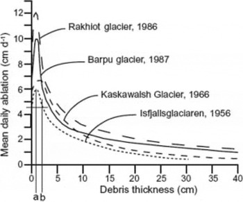
Fig. 1. Examples of empirical measurements of the relationship between debris thickness and ice ablation rate on sample glaciers (redrawn from Reference Mattson, Gardner and YoungMattson and others 1993): Rakhiot glacier, Punjab Himalaya; Barpu glacier, Karakoram Himalaya, Pakistan; Kaskawalsh Glacier, Yukon, Canada; and Isfjallsglaciaren, Sweden. Note the variation in (a) the thickness beneath which maximum melt occurs and (b) the thickness at which melt becomes inhibited compared to that of clean ice on different glaciers (indicated for Isfjallsglaciaren).

Previous Work

Sub-debris melt rate, M (surface lowering in m s⁻¹), can be calculated as:

(1)

where Q _m is downward energy flux at the base of the layer (W m⁻²), ρ _i is the density of ice (900 kg m⁻³) and L_f is the latent heat of fusion (334 kJ kg⁻¹). As the energy flux through the debris layer is dominated by heat conduction down a vertical temperature gradient from the debris surface to the ice, Q _m is given by the conductive heat flux, Q_c , across the debris–ice interface. Q _c can be derived from the one-dimensional heat-flux equation for conduction:

(2)

in which k is the thermal conductivity of the debris layer (W m⁻¹ K⁻¹) and T is temperature within the layer (K) at a point z within the layer (m). Previous workers (Reference KrausKraus, 1975; Reference Nakawo and YoungNakawo and Young, 1981) have made the appealing simplification of taking the temperature gradient between the upper and lower surfaces of the debris layer to be linear. This means that Equation (2) can be written as a function of the steady-state surface (T _s) and ice (T _i) temperatures (K) and debris thickness, h _d (m):

(3)

This simplification rests on the assumption that the debris layer is in thermal equilibrium, i.e. the heat stored in the layer is constant over time, and accepting it means that Q _c at the debris surface is the same as at the ice interface. However, surface temperatures of supraglacial debris vary on a variety of timescales in response to changing meteorological conditions, and this drives ongoing changes in the thermal regime of the debris layer. Reference Nakawo and YoungNakawo and Young (1981) calculated daytime and night-time ablation from meteorological data, assuming steady state was attained over these timescales, but data from vertical temperature profiles through supraglacial debris demonstrate that this assumption is not valid (Reference NicholsonNicholson, 2004). Under stable weather conditions the thermal regime of the debris is dominated by the diurnal cycle (Fig. 2a; see also Reference Conway and RasmussenConway and Rasmussen, 2000; Reference NicholsonNicholson, 2004; cf. Reference HumlumHumlum, 1997), so in debris cover of more than a few centimetres in thickness, equilibrium within the debris layer cannot be expected over time intervals of anything less than 24 hours. Consequently, the assumption of a linear temperature gradient will not be met on sub-diurnal timescales, but is much more likely to apply on a 24 hour timescale (Reference Conway and RasmussenConway and Rasmussen, 2000; Fig. 2b).

Fig. 2. Diurnal temperature oscillations in debris at progressively greater depths measured at Ngozumpa Glacier, Khumbu Himal, Nepal. Temperature waves penetrate with decreasing amplitude and increasing lag (a), resulting in variations and marked nonlinearity in the instantaneous vertical temperature profiles (b). The daily mean temperature profile, however, is close to linear, as was also found by Reference Conway and RasmussenConway and Rasmussen (2000). Vertical lines in (a) mark the times of profiles shown in (b).

While Reference Nakawo and YoungNakawo and Young’s (1981) model results show general agreement with their empirical measurements, the effect of thermal disequilibrium, i.e. changes in the amount of heat stored in the debris layer within the calculation time interval, results in over-prediction of melt rates at night and under-prediction during the day. Reference Nakawo and YoungNakawo and Young’s (1981) daytime and night-time calculated melt rates differed from the measured melt rates by up to ~80% in individual cases, although the model results were generally within 30% of the measured values. Reference Kayastha, Takeuchi, Nakawo and AgetaKayastha and others (2000) calculated melt by applying Nakawo and Young’s method to continuous measurements over the course of the day, and found calculated values of melt rate beneath a 0.1 m thick debris layer up to double those measured in the field. This overshoot is understandable because the assumption of an instantaneously linear temperature gradient does not account for the inversion of the temperature gradient that occurs at night, at least in the near subsurface, which results in heat flux towards the debris surface rather than towards the ice, such that initial energy inputs are used to raise the debris temperature rather than to melt ice. The maximum debris thickness used in these comparisons of modelled and measured melt was ~10 cm. Some glaciers support debris an order of magnitude thicker than this, and it should be noted that the effect of thermal disequilibrium, and thus the importance of choosing an appropriate time interval for analysis, is likely to be more pronounced in thicker debris layers. In the light of this we propose that a timescale of 24 hours is the minimum interval over which to employ the simplified heat-flux model (Equation (3)).

Solution of Equation (3) requires that debris surface temperatures are known, and, due to the difficulties of obtaining representative field measurements for the entire debris-covered surface, most published studies can only calculate melt at a small number of experimental sites. For example, Reference Kayastha, Takeuchi, Nakawo and AgetaKayastha and others (2000) measured ablation below seven different debris thicknesses over a 12 day period on Khumbu Glacier, Nepal, but were only able to compare these data to calculated melt for the single site at which surface temperature was measured. The use of thermal band satellite data to determine T _s has been proposed (Reference Nakawo and RanaNakawo and Rana, 1999), but the utility of such data is limited by the fact that they yield only instantaneous temperatures which will not be applicable over longer timescales (Reference Conway and RasmussenConway and Rasmussen, 2000).

In their original paper, Reference Nakawo and YoungNakawo and Young (1981) circumvented the problem of requiring Ts in Equation (3), by using meteorological data to solve an equilibrium surface energy-balance equation:

(4)

where Q _s, Q _l, Q _h, Q _e and Q _c (all in W m⁻²) are net shortwave radiation flux, net longwave radiation flux, net sensible heat flux, net latent heat flux and conductive heat flux into the debris, respectively, with all terms taken to be positive towards the debris surface. Debris surface temperature, T_s , contributes to all terms except Q_s, but if all other variables can be measured or estimated, T_s remains the only unknown. Although their method was not clearly stated, Nakawo and Young found an approximate analytical solution that eliminated T _s and expressed Q _c in terms of the known meteorological variables. This surface energy-balance model is appealing as it uses meteorological data, which are more easily obtainable than surface temperature data, and are often available from existing meteorological stations. However, it would be preferable to have a method that finds an exact solution of the surface energy-balance and yields an explicit value of T _s, as this would enable the individual surface energy-balance terms to be fully calculated. At present, this complete apportionment of the surface energy balance into its constituent energy source components has only been possible for experimental sites at which continuous surface temperature measurements have been made (Reference Kayastha, Takeuchi, Nakawo and AgetaKayastha and others, 2000; Reference Takeuchi, Kayastha and NakawoTakeuchi and others, 2000).

Modelling Ablation beneath a Debris Layer

Here we describe a method for calculating sub-debris melt using diurnally averaged meteorological data and evaluate its performance by comparison with empirical measurements of melt. The energy-balance equation, Equation (4), is solved numerically, to obtain an explicit value for mean daily debris surface temperature, allowing all terms of the energy balance to be quantified. Although Reference Purdie and FitzharrisPurdie and Fitzharris (1999) give a method for incorporating heat delivered by precipitation in the surface energy balance, this is not included here, as direct heat exchanges from infiltrated rainfall have been shown to have negligible effect on the melt of debris-covered ice (Reference Sakai, Fujita and KubotaSakai and others, 2004).

The radiative components of Equation (4) are expressed as:

(5)

(6)

where Q′ is incoming shortwave radiation (W m⁻²), α is albedo, l* is incoming longwave radiation (W m⁻²), ε is the emissivity of the debris surface (taken to be 0.95), α is the Stefan–Boltzmann constant (5.67 × 10⁻⁸ W m⁻² K⁻⁴) and T _s is the debris surface temperature (K). Turbulent heat-flux components are parameterized using bulk transfer coefficients following Reference PatersonPaterson (1994):

(7)

(8)

where ρ ₀ is the density of air at standard sea-level pressure (1.29 kg m⁻³), P is air pressure at the site (Pa), P ₀ is standard air pressure at sea level (1.013 × 10⁵Pa), c is the specific heat capacity of air (1010J kg⁻¹ K⁻¹), u is wind speed (m s⁻¹), Tz is air temperature (K) at height z (m), T _s is debris surface temperature (K), L _e is latent heat of evaporation of water (2.49 × 10⁶J kg⁻¹), e_z and e_s are the vapour pressure (Pa) at height z and at the upper debris surface, respectively, and A is a dimensionless transfer coefficient given as:

(9)

where k _* is von Kármán’s constant, z is the height of meteorological measurements and z ₀ is the surface roughness length, here taken to be 0.01 m, on the basis of values for very rough ice and sastrugi (Reference BrockBrock, 1997) and previous calculations over debris-covered surfaces (Reference Takeuchi, Kayastha and NakawoTakeuchi and others, 2000).

All independent variables are 24 hour means, and the temperature at the ice–debris interface is assumed constant at 0°C. Debris surface temperature, T _s, appears explicitly in the outgoing longwave, sensible-heat and conductive terms, and implicitly (through its influence on saturation vapour pressure) in the latent-heat term. The value of T _s that satisfies Equation (4) for given meteorological conditions is found numerically by iteration. The resulting daily mean surface temperature is then used to calculate melt from Equations (2) and (1) for prescribed debris thickness and debris thermal properties. The moisture content of the debris layer will exert a strong influence on its thermal properties, yet this property is difficult to determine for an entire glacier surface and is unlikely to be known in any practical application of the model, hence, in this work we tackled the unknown nature of the moisture content of the debris by considering the two limiting cases of the debris cover being either completely dry or fully saturated. For each set of input meteorological parameters two østrem curves were produced; one using the optical and thermal properties of dry debris and the other using the properties of saturated debris. For dry conditions Q _e is 0, and for saturated conditions Q _e is calculated using the saturation vapour pressure for the debris surface temperature.

Comparison of Calculated and Observed Melt Rates

Model performance was evaluated by comparison of calculated melt rates with sub-debris melt rates measured over periods of 4–11 days at Ghiacciaio del Belvedere, Italian Alps (45°57′N, 4°34′E; 2000 m a.s.l.), and Larsbreen, Svalbard (78°11′N, 15°33′E; 200 m a.s.l.). Plots of varying debris thickness were prepared by clearing the ice surface of all debris, levelling the ice surface and inserting a 12 mm diameter white plastic ablation stake into the ice before replacing the local debris to the required depth. As far as possible, debris was replaced in its original stratigraphic position. At Larsbreen, melt rates were measured at 11 experimental plots of varying debris thickness from 9 to 20 July 2002, and at Ghiacciaio del Belvedere five plots were monitored from 6 to 10 August 2003. Over the course of the measurement periods, differential ablation caused the originally level ice surfaces to become uneven, resulting in local changes in debris thickness during the experiments. In order to minimize disturbance to the system, the debris cover could not be excavated daily, so it is impossible to determine the actual melt amounts or debris thickness on each day. Hence, daily ablation at each site was estimated from the measured change in ice surface from the beginning to the end of the experiment, divided by the number of days of the measurement period. The corresponding debris thickness was taken to be the mean of initial and final measured thickness, with maximum measurement error on all measurements estimated to be 5 mm.

Automatic weather stations were used to record incoming shortwave radiation (Kipp and Zonen CM3 pyramometer; 0.3–2.8 μm), 1.5 m air temperature (T _a) and relative humidity (RH) (Campbell CS500) and wind speed (Vector Instruments A100R switching anemometer). Incoming longwave radiation was measured using a Kipp and Zonen CG1 pyrgeometer (4.5–42 μm) at Ghiacciaio del Belvedere, and at Larsbreen was calculated as a residual using continuous measurements of shortwave radiation (Kipp and Zonen NR-lite), net shortwave radiation and surface temperature (from which outgoing longwave radiation was calculated). Vapour pressure was calculated from relative humidity and air temperature using the Clausius–Clapeyron formula. Atmospheric pressure at the site was not measured directly, but was taken to be that of a standard atmosphere for the altitude of the field site.

Debris surface albedo for each glacier was measured using a hand-held Kipp and Zonen CM3 radiometer. Spot measurements of albedo at wet and dry debris surfaces (n = 551 at Larsbreen and 136 at Ghiacciaio del Belvedere) were made at intervals during daylight hours, and averaged to determine the characteristic mean daily albedo for these two surface states (Table 1). The thermal conductivity of the debris, k, was calculated using the method of Reference Conway and RasmussenConway and Rasmussen (2000). Assuming all heat flux to occur by conduction, and thermal conductivity to be constant with depth, this method uses time series of vertical temperature profiles within the debris to determine the apparent thermal diffusivity of the debris (κ) using a one-dimensional thermal diffusion equation:

(10)

where T is debris temperature, t is time and z is the vertical coordinate. A value of κ at each thermistor can thus be determined as the gradient of the best-fit line of the first derivative of temperature with time plotted against the second derivative of temperature with depth, with the associated standard error on the best-fit line. Then k can be determined from κ (m s⁻²) and the volumetric heat capacity:

(11)

where c _d and ρ _d are the specific heat capacity and density of the debris, φ is the porosity and c _v and ρ _v are the specific heat capacity and density of the void filler within the debris. Temperature profiles were measured at 30 min intervals using vertical arrays of thermistors attached to Gemini Tinytag data loggers. At Larsbreen eight loggers were used over 0.65 m debris thickness, and at Ghiacciaio del Belvedere four loggers were used over 0.27 m. The uppermost thermistor was covered with a layer of locally derived fine particles to avoid direct exposure to sunlight. Temperature derivatives were calculated from thermistor data using a standard centred differencing scheme for unevenly spaced points, applied to a portion of the temperature time series that indicated the debris temperatures had stabilized since the emplacement of the thermistors. Within these time series, we choose periods of stable conditions where the temperature records are least noisy and follow a consistent diurnal oscillation with increasing lag and decreasing amplitude with depth, as these represent the best conditions for applying this method. For Larsbreen the chosen analysis period was 22–25 July 2002 (4 days), and for Ghiacciaio del Belvedere the period was 7–11 August 2003 (5 days). Following Reference Conway and RasmussenConway and Rasmussen (2000), a representative value of κ for the whole layer was found by averaging the values from each thermistor. Depth-averaged κ for Larsbreen and Ghiacciaio del Belvedere are 0.30 ± 0.05 mm² s⁻¹ and 0.38 ± 0.02 mm² s⁻¹, respectively. The volumetric heat capacity was calculated using published values of ρd (2700 kg m⁻¹) and c_d (900 J kg⁻¹ K⁻¹) for the sedimentary lithology of the Larsbreen region and 890 J kg⁻¹ K⁻¹ for the metamorphic lithology of the Ghiacciaio del Belvedere region, and porosity was estimated from matrix particle size determined by laser diffraction using a Coulter LS230 (Table 1). Maximum and minimum values of thermal conductivity were calculated for supraglacial debris at each glacier using a weighted-average volumetric heat capacity based on the limiting cases of water-filled pore spaces (‘wet’) and air-filled pores (‘dry’), using standard values of density and specific heat capacity for air and water void fillers. The value of k _dry was first calculated using Equation (11) with the depth-averaged κ and volumetric heat capacity of air-filled voids. From this, thermal conductivity of the solid rock, k _s, was derived using a parallel-flow model for a composite body; k _wet was calculated from k _s using an empirical function (Reference FaroukiFarouki, 1986) that has been shown to give good estimates of saturated thermal conductivity:

(12)

where k _w is the thermal conductivity of water and x is the volume fraction of each component. Thermal conductivity values calculated for both wet and dry conditions at both glaciers are presented in Table 1. Debris temperature data collected in order to calculate κ were also used to compute daily mean temperature profiles at both sites. The minimum r value for linear regression on mean daily temperature profiles was 0.97, confirming the linearity of temperature gradients through the supraglacial debris on a 24 hour timescale.

Table 1. Debris properties for Larsbreen and Ghiacciaio del Belvedere; c _d and ρ _d values compiled from Reference Robinson and CoruhRobinson and Coruh (1988) and Reference LideLide (2004). Bulk volumetric heat capacity calculated from the density and specific heat capacity of the rock and void filler components was assumed to have an error of 10% which was incorporated in the calculation of k

Comparisons of modelled and measured melt at Ghiacciaio del Belvedere and Larsbreen are presented in Figures 3 and 4. Four of the five plots at Ghiacciaio del Belvedere were freely drained throughout (although the debris was damp at depth), but, at the end of the experiment, one plot (h _d = 0.021 m) was found to be saturated, with water ponded at the ice–debris interface. At the freely drained plots, melt rates calculated using values of k appropriate for dry debris are within 27% of measured values, and, at the saturated plot, calculated melt rate using values of k appropriate for saturated debris is within 5% of the measured value (Fig. 3). The close match between measured and modelled melt rate at the only site where moisture content is well known suggests that the model performs well when debris properties are well known. In most cases, however, the model output can only approximate the measured melt values due to the unknown specific moisture content of each experimental site. At Larsbreen, the measured values are most closely approximated by model results for dry debris (Fig. 4), despite the fact that the debris was observed to be saturated where the layer was <0.1 m, and moist where it was thicker, so the measurement would be expected to plot closer to the modelled results for saturated debris. This pattern suggests that the model systematically over-predicts ablation in this environment. Inspection of the calculated surface temperature shows that the modelled values correspond closely to those calculated by the model for saturated debris conditions (Fig. 5b). Thus, the overprediction is probably due to the assumption that ice is at 0°C throughout, such that all conductive heat flux towards the ice is used for melt, which may not be the case at Larsbreen. Conductive heat flux into the ice could not be incorporated in the modelled results, because temperature gradients within the ice were not recorded.

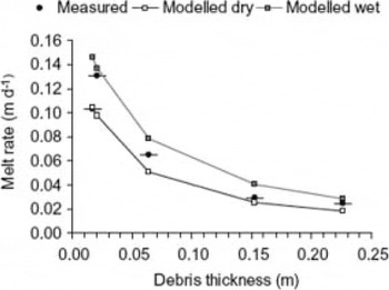
Fig. 3. Comparison of modelled and measured melt rates over a 4 day period at Ghiacciaio del Belvedere.

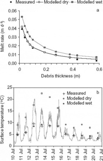
Fig. 4. (a) Comparison of modelled and measured melt rates over an 11 day period at Larsbreen. (b) Comparison of surface temperature modelled for wet debris with surface temperature recorded at an experimental plot with a 10 cm thick wet debris layer shows good agreement, suggesting that measured melt rates fall below the modelled melt rate due to heat being conducted into the ice rather than being used for melt. The grey line shows the continuous temperature measurement; the crosses are the daily mean of the measured values.

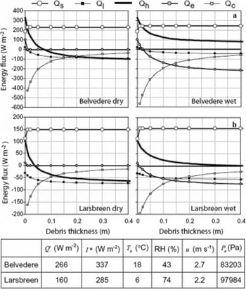
Fig. 5. Energy-balance components calculated for bare ice and for debris-covered ice using modelled surface temperatures for wet and dry debris at Ghiacciaio del Belvedere and Larsbreen.

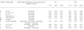
Discrepancies between the measured melt rates and the model results can be attributed to a variety of sources of error. Measurement errors associated with the meteorological instruments are ±10% for the radiometers, ±2% for relative humidity and ±1% for air temperature and wind speed (although the error in wind speed can be up to 33% at stalling speed). Air pressure was only approximated in the model runs carried out in this work, and error on this value is estimated to be ±2%. Maximum error in calculated melt rate, determined using the root-sum-squares method is 18% at Belvedere and 25% at Larsbreen, the majority of which can be attributed to error in the calculated thermal conductivity value. Sensitivity analysis shows the model to be most sensitive to air temperature, as would be expected. Changing other input parameters individually results in maximum percentage changes in melt that are considerably smaller than the percentage change in the input parameter (Table 2). For example, although surface roughness length is one of the more poorly parameterized components of the model (taken as a standard value in this work), the effect of a change in z0 on melt rate is very small; a 10% variation in z ₀ generally results in only a 1–2% change in modelled melt rate (Reference NicholsonNicholson, 2004; Table 2), suggesting that this crude parameterization has little effect on model output. Despite these sources of model uncertainty, our results indicate that the model, as currently formulated, performs well for summer conditions on Ghiacciaio del Belvedere but needs the incorporation of conductive heat flux into the ice where ice is colder, as in the case of Larsbreen.

Table 2. Summary of sensitivity analysis. Each input variable was perturbed by ±1% from 10–12 selected values spanning the range of that parameter. Values quoted are the maximum absolute percentage change (quoted to two decimal places) in melt rate in response to a 1% change in the individual input parameter. Column 2 indicates how melt rate responds to an increase in the input parameter, and whether or not the sense of this response changes with increasing debris thickness

Discussion

Some published empirical østrem curves show a ‘rising limb’ for very light debris load, where melting increases with increasing debris thickness (e.g. Reference KonovalovKonovalov, 2000; Reference Tangborn and RanaTangborn and Rana, 2000; Fig. 1). Although our model output provides a good match of the form of the østrem curve, showing an asymptotic decline in melt with increasing debris thickness, it does not mimic this rising limb, and instead predicts falling melt rates with increasing debris thickness, even for infinitesimally thin debris. Our model represents even a very small amount of surface debris as a continuous layer of uniform thickness, but in reality a light debris load consists of scattered particles, or ‘clots’ of debris (Adhikari and others, 1997, 2000). In this case the surface albedo is a function of the proportion of the surface that is debris-covered, and this may account for the observed ‘rising limb’. This can be simulated in the model by linearly varying surface albedo between the value for clean ice (h _d = 0) and that for supraglacial debris at some specified minimum thickness for a continuous debris layer.

Explicit calculation of surface temperature not only provides an alternative means of evaluating model performance as in Figure 4b, but also allows us to explore how energy-flux partitioning of the surface energy-balance components changes between clean ice and debris-covered ice, and how surface debris affects surface energy balance under the influence of contrasting climatic conditions. Meteorological conditions at Larsbreen contribute significantly lower amounts of energy than those at Ghiacciaio del Belvedere, where mean daily surface energy flux at a 0°C ice surface is more than three times that at Larsbreen. Surface energy fluxes associated with averaged midsummer conditions at Ghiacciaio del Belvedere (measured in August 2003) and at Larsbreen (measured in July 2002) are shown in Figure 5a and b, respectively.

In the case of the temperate Ghiacciaio del Belvedere, it can be seen that the energy fluxes over bare ice are all positive, with the largest positive energy flux being sensible heat. In the presence of debris cover, the dominant energy contribution switches from sensible heat flux to shortwave radiation in response to the lower albedo and higher debris-surface temperatures. In the case of dry debris cover, sensible heat flux becomes negative at greater debris thicknesses, because of higher debris-surface temperatures. Longwave radiation also becomes negative even for thin debris cover. Under wet debris conditions, sensible heat flux remains a positive flux and longwave radiation is less negative, because the debris surface is cooled by latent-heat losses. These approach the same magnitude as the positive shortwave contribution as debris thickness increases. The cooler summer climate on Larsbreen means that over bare ice longwave flux is negative, despite the high relative humidity, and the sensible heat fluxes, although positive, are smaller than the shortwave radiation contribution. In general, the fluxes respond in the same way to increasing debris thickness as they do at Ghiacciaio del Belvedere, but the lower air temperature means that the turbulent fluxes become negative more readily with increasing debris thickness. In both cases, the proportional decrease in sensible heat contributions caused by dry debris cover is greater than the proportional increase in shortwave radiation contributions, but this is reversed in the case of wet debris cover when the albedo difference between ice and debris-covered ice is maximized and latent-heat exchange cools the surface, thus maintaining a stronger temperature gradient between the surface and a warmer atmosphere.

At Ghiacciaio del Belvedere, a 1 cm debris cover reduces the energy flux available for melt by 33% if the debris is dry, and by 11% if the debris is wet, while at Larsbreen the same debris thickness reduces the energy flux available for melt by only 17% where debris is dry, and increases the energy flux by 2% where wet, in comparison to clean ice. The pattern of difference between the two environments is not markedly changed if both sets of fluxes are analyzed with a standard debris cover of common thermal and optical properties. Thus the contrasts evident in Figure 5 are more strongly controlled by marked differences in meteorological conditions than contrasting debris properties at the two glaciers.

Thin debris cover only causes accelerated melt compared to that of clean ice in the case of wet debris conditions at Larsbreen. In this type of summer climate where humidity is relatively high and air temperature relatively low, the increase in shortwave receipts at the surface is only partially offset by reduced sensible-heat flux and slightly negative latent-heat flux, such that the overall energy available for melt (assuming no conduction into the ice beneath) increases compared to the clean-ice case. These data suggest that the likelihood that thin debris cover will accelerate melt is maximized under cooler, cloudier conditions. Thus we can see that while thick surface debris cover tends to inhibit melt under all conditions, the influence of a thin debris cover on melt rate compared to that of clean ice may tend towards a negative feedback, inhibiting melt in conditions when total energy flux to a bare ice surface is high, but accelerating melt rate in conditions when total energy flux to a bare ice surface is low.

The diurnally averaged melt model rarely calculates accelerated melt rate even beneath thin debris. This is because diurnally averaged meteorological inputs mask cooler parts of the diurnal cycle during which the presence of thin debris may accelerate melt. In effect, the presence of thin debris may accelerate melt more by virtue of extending the duration of melt within a day than by accelerating the melt rate under the optimal ablation conditions during the warmest part of the day (generally early afternoon). Thus, if one is interested in modelling the effects of thin debris cover, such as might result from a light ashfall, on ablation, the temporally averaged method presented here may produce misleading results. Where debris cover is very thin, its heat storage capacity is small and thermal equilibrium will be achieved more quickly. Thus, it may be more appropriate to average input data and calculate melt rates on shorter temporal scales. However, debris-covered glaciers tend to support supraglacial debris of the order of decimetres to metres in thickness, and in such cases diurnal timeaveraging is a distinct advantage. The results presented here show our model performs well over a broad range of debris thicknesses, and so will be applicable to the majority of debris-covered glaciers.

The principal limitation of applying a meteorological melt model as proposed here is obtaining high-quality input parameters. Field determination of debris properties is especially problematic, and more detailed work to determine the accuracy of the techniques is required. The results presented here, however, provide support for the approach employed by Reference Conway and RasmussenConway and Rasmussen (2000) for determining debris thermal conductivity. Determining the turbulent fluxes at a debris-covered ice surface remains largely unexplored and at present is the least constrained area of the model. As currently formulated, our model does not account for the fact that cold surface ice can be a major heat sink, particularly early in the melt season in cold environments (Reference HockHock, 2003). Therefore a two-layer model construction, incorporating conduction of heat into the ice, will be necessary if the model is to be applied at the margins of the melt season or in polar environments.

Conclusions

The model described in this paper allows melt rates beneath debris layers of arbitrary thickness to be calculated from daily mean meteorological data and basic debris layer characteristics (thickness and apparent thermal diffusivity). The model assumes that (1) daily mean temperature gradients are linear and (2) there is negligible net change in heat storage on diurnal timescales; these assumptions are valid for summer conditions at both our study sites. The assumption that the underlying ice is at the melting point is valid for temperate glaciers in summer, but may yield erroneous results for polythermal glaciers, and on all glaciers in early spring before near-surface ice cooled during the winter is raised to melting point.

On the basis of the data presented here, despite numerous simplifications, the model performs well and provides a good match with observed values, suggesting it can produce reliable estimates of ablation rate beneath debris layers of several decimetres in thickness. This is a useful improvement on previous model incarnations which are inappropriate for thick debris cover where changes in heat stored in the debris cover over the course of a day result in non-linear instantaneous vertical temperature gradients. In addition, the model presented here allows comparison of regional surface energy fluxes, so the influence of supraglacial debris cover can be assessed in the context of regional climatic conditions.