


1. Introduction
Recent measurements (Reference Abdalati and KrabillKrabill and others, 1999, Reference Krabill2000) show that most coastal parts of the Greenland ice sheet thinned between 1993/94 and 1998/99. Summer temperatures during this period were warm, compared to a 20 year climatology for the period 1979–99 (Reference KrabillKrabill and others 2000), and melt was observed to increase slightly over the same time period (Reference Abdalati and SteffenAbdalati and Steffen, 2001). This probably caused some of the observed thinning. But the amount of increased melt attributable to the higher summer temperatures, calculated by the positive-degree-day method (Reference ReehReeh,1991; Reference BraithwaiteBraithwaite, 1995), can explain only part of the observed thinning (Reference AbdalatiAbdalati and others2001). The number, N, of positive degree days (PDDs) for each month was calculated for nearby coastal weather stations as the integral over time of all air temperatures >0°C. Comparison of these values during the period of observed thinning with long-term averages gives the PDD anomaly, which was extrapolated inland assuming linear decrease with surface elevation to zero at the inland limit of summer melting. The resulting values were multiplied by a coefficient (k = 9 mm PDD−1) to give estimates of near-coastal surface lowering caused by higher-than-normal surface melting. These estimates show good agreement with observed elevation changes (Reference AbdalatiAbdalati and others2001) for some glaciers and stagnant ice margins, but they are not large enough to explain the higher thinning rates.
Jakobshavn Isbræ was one of the few surveyed glaciers to thicken between the 1993 and 1998 surveys, despite a local positive PDD anomaly (Reference AbdalatiAbdalati and others, 2001). Airborne laser-altimeter surveys along a 120 km profile in the Jakobshavn basin have been made almost every year since 1991 by NASA’s Airborne Topographic Mapper (ATM). These show slow, sporadic thickening between 1991 and1997, suggesting a small positive mass balance in broad agreement with the previous balance estimates. Since 1997, however, there has been sustained thinning of several m a−1 within 20 km of the ice front, with lower rates of thinning further inland. Velocity measurements made during various periods since the 1960s show little variation (Reference Carbonnell and BauerCarbonnell and Bauer, 1968; Reference Lingle, Hughes and KollmeyerLingle and others1981; Reference Echelmeyer and HarrisonEchelmeyer and Harrison, 1990; Reference Fastook, Brecher and HughesFastook and others1995; Reference Abdalati and KrabillAbdalati and Krabill, 1999) and there is negligible seasonal change (Reference Echelmeyer and HarrisonEchelmeyer and Harrison, 1990). However, the recent thinning may indicate a change in glacier dynamics that will result in another retreat of the ice front. Consequently, we attempt here to infer how much of the observed thinning since 1997 was caused by increased creep thinning of the glacier, in order to reveal the spatial and temporal pattern of dynamic change.
Jakobshavn Isbræ is the most active glacier in Greenland, draining approximately 7% of the ice sheet, with an annual discharge of 27–31 km3 of ice at speeds up to 7 km a−1 (Reference Echelmeyer, Harrison, Clarke and BensonEchelmeyer and others1992; Reference WeidickWeidick, 1995), making it the fastest glacier in the world. Most of its catchment area lies within the dry-snow zone of the ice sheet, but it includes large regions within the percolation, soaked and ablation zones, with melt rates of several m a−1 near the calving front. Many large lakes with depths up to several meters form during most summers in the percolation and ablation zones, and in situ measurements and frequently repeated laser-altimetry data show that some empty very rapidly. The calving front retreated 30 km between 1850 and 1964 but it has occupied approximately the same location since (Reference WeidickWeidick, 1995; Reference HughesHughes, 1998, fig. 1.5; Reference Sohn, Jezek and van der VeenSohn and others1998). Balance calculations for 1985/86 by Reference Echelmeyer, Harrison, Clarke and BensonEchelmeyer and others, (1992) suggest that total loss by surface and basal melt and ice discharge is slightly less than total accumulation within the drainage basin, but not by more than errors in the estimates.
2. Measurements
2.1. Airborne Topographic Mapper
Measurements of ice-surface elevations along flight-lines over Jakobshavn Isbræ were made during most years since 1991 using the NASA ATM, a scanning laser altimeter that measures the surface elevation of many 1 m laser footprints within a 140–400 m wide swath beneath the aircraft to an accuracy of about 10 cm (Reference Krabill, Thomas, Martin, Swift and FrederickKrabill and others, 1995, Reference Krabill2002). A major survey was completed in 1997, along a grid pattern of flight-lines, but one profile was resurveyed almost every year (Fig. 1). It runs east–west along the lowest reaches of the glacier, but then moves to the north of the main trunk of the glacier to cross the catchment basin in a northeast direction. The most complete coverage of this line was obtained during May 1997, so each laser-footprint elevation from other surveys was compared with those from the 1997 survey within a horizontal radius of 1 m, to obtain estimates of the elevation change (ΔS) between surveys. All elevations were measured with respect to the World Geodetic System 1984 (WGS84) ellipsoid, which is about 26 m below sea level near Jakobshavn Isbræ, and we use the same reference level here.

Fig. 1. A map of theJakobshavn Isbræ region, showing flight-lines with the ATM, locations of coastal weather stations (CWS) at Egedesminde (E) and Ilulissat (I) and of automatic weather stations (AWS) on the ice sheet at JAR-1, -2 and -3 (J1, J2 and J3), Swiss Camp (S) and Crawford Point (C).TheATM flight-linethat was resurveyed most frequently between 1991 and 2001 (“main line”) is highlighted.
Figure 2 shows observed elevation changes derived in this way. The high spatial variability of ΔS at lower elevations is caused by large changes in surface elevations at a fixed point as crevasses and ice blocks move forward with the glacier. Elevation changes averaged over longer sections of the profile are more subdued and are thus likely to give a good indication of net changes. Below about 110 m elevation, much of the glacier is floating, but with partially grounded areas. The entire floating tongue is intensively crevassed, and the surface is particularly rough, making local ΔS estimates very noisy. In addition, glacier advances and retreats result in very large, spurious values of ΔS. Consequently, in this area we estimated elevation changes for two adjacent 2 km sections ofthe glacierbycomparingaverageelevations for a section, derived from each ATM survey. The section nearest the ice front (Fig. 2) has a near-horizontal surface and is probably floating. The adjacent section straddles a small dome that probably marks an area of local grounding, or “ice rumples”. Repeat coverage by the ATM survey was sparse before1993, after which there was progressive thickening of the glacier at all elevations until 1997, with a marked change to rapid thinning afterwards. Although these results apply only to the surveyed traverse, they show broad agreement with estimates of ΔS derived for locations where each year’s flight-lines crossed the 1997 grid survey. However, these “crossing-point” estimates are very noisy because they apply to small areas of the very rough glacier surface, with each year’s survey over different roughness samples.

Fig. 2. Main-line elevation profile with the total elevation change (ΔS) for each survey compared to the 1997 survey. In order to subdue ΔS “noise”associated with crevasses and ice pinnacles, the plotted values of ΔS are averages over about 300 m of flight-line.
2.2. Automatic weather station and in situ measurements
During the time period covered by the surveys, we also have measurements of snow accumulation and air temperature from Swiss Camp, to the north of the glacier, situated close to the equilibrium line (where the surface mass balance is zero) at an elevation of about 1180 m. In the late 1990s, these measurements were augmented by similar ones from a total of five automatic weather stations (AWSs) at elevations of 327–2022 m (Reference Steffen and BoxSteffen and Box, 2001). Each spring, between 20 and 25 May, snow depth and density were measured at Swiss Camp (S in Fig. 1), and at the AWSs at JAR (Jakobshavn ablation region) -1, -2 and -3 and Crawford Point1 and 2. The JAR stations are located in the ablation regions, and the measured snow cover at that date represents the winter accumulation. At Swiss Camp (equilibrium-line altitude) the reference surface height from the previous summer was derived from the acoustic height instruments at the AWS. At Crawford Point 1 and 2 the snow pit was analyzed and the last summer horizon was identified using grain-size analysis. The level was verified with the acoustic height measurements which record the surface height change throughout the year on an hourly basis. The Crawford Point stations, at 1990 and 2022 m elevation, are very close together, and we averaged observations from these stations and assigned them to an elevation of 2000 m (C in Fig. 1). At all AWSs, temperatures were sampled every 10 s, and we used the hourly averages of these measurements. On the coast, there are also long time series of weather observations from Egedesminde and Ilulissat (Fig. 1). Although Ilulissat is closer to the glacier, measurements were not continuous through our observation period, so we use the Egedesminde data in this investigation.
3. Analysis
3.1. Theoretical concept
The vertically integrated equation of continuity for an ice column of thickness H at a fixed location (e.g.Reference Van der VeenVan der Veen, 1999, p.154), modified to take account of flowline divergence and firn densification, can be written to give the rate at which the surface elevation increases with time:
where A is the snowfall expressed as a thickness of surface snow per unit time (this includes all snow precipitation that is not removed by drifting, and is different from net surface mass balance), M is the melt rate expressed as a thickness of surface snow or ice per unit time, and includes losses by evaporation, with subscripts s and b the surface and base of the ice column respectively, V
b is the upward vertical velocity of the bed beneath the ice, V
d is the downward surface velocity caused by snow densification, ![]() is the depth-averaged vertical creep rate, which includes the effects of longitudinal strain and of lateral divergence/convergence, U is the depth-averaged horizontal velocity, H is ice thickness, assumed to vary only in the ice-flow direction, and ∂H/∂x is the ice-thickness gradient taken along the direction of motion.
is the depth-averaged vertical creep rate, which includes the effects of longitudinal strain and of lateral divergence/convergence, U is the depth-averaged horizontal velocity, H is ice thickness, assumed to vary only in the ice-flow direction, and ∂H/∂x is the ice-thickness gradient taken along the direction of motion.
The effects of basal melting M
b and crustal motion V
b are generally very small and can be neglected. Moreover, the dynamic behavior of the glacier is described by the term ![]() , which is negative for dynamic thinning, so, for convenience, we define the rate of dynamic thinning as
, which is negative for dynamic thinning, so, for convenience, we define the rate of dynamic thinning as ![]() . Equation (1) then becomes:
. Equation (1) then becomes:
During a specific time period ΔT

and the change in surface elevation during a time interval ΔT is:

where the subscript m denotes long-term averages, and the primed terms are differences between values during ΔT and the long-term averages. Over short time periods, values of A ′, M ′ and V ′ are determined by the weather, and can differ widely from year to year. In addition, they may have longer-period cycles associated, for instance, with the North Atlantic Oscillation (NAO). By contrast, D ′ is determined by glacier dynamics, and short-term changes are generally small, except during glacier surges or the retreat of tidewater glaciers. Our observations of a large, sustained change in ∂S/∂t on Jakobshavn Isbræ suggest a change in dynamics, and our objective here is to use available data to solve Equation (3) in order to infer the magnitude and spatial and temporal patterns of D ′. For this purpose, we assume (∂S/∂t)m = 0, implying the glacier has been in steady state for the past few decades, as suggested by observations showing the ice front has been in approximately the same location since 1964 and by the 1985/86 measurements of Reference Echelmeyer, Harrison, Clarke and BensonEchelmeyer and others, (1992). The repeat ATM surveys give measurements of ΔS for a range of surface elevations from near sea level to almost 2000 m based on comparisons of surveys made between 1991 and 2001 with one in 1997.We also need estimates of A ′, M ′ and V ′.
3.2. Snow accumulation and compaction, and surface melting
For each year since 1991, we estimated values of A in the ablation zone based on the depth of snow accumulated over winter at Swiss Camp from observations made during May each year, implicitly neglecting loss by melting during the winter. Over several years in the late 1990s additional weather stations were installed, so for the year May 2000–May 2001 we also have accumulation estimates at the five AWSs between 327 and 2000 m ellipsoid elevation, and we adjusted the Swiss Camp observations to other elevations for each of the years 1991–2001, assuming an elevation dependence similar to that during 2000/01 (Table 1). We used these values as the annual accumulated snow depth at each station.
Table 1 Values of the PDD factor (k) and snowfall (A) at sites nearJakobshavn Isbræ

Both surface melting (M s) and snow compaction (V d) are strongly affected by temperature, so we assumed a simple relationship between (M s + V d) and the number, N, of PDDs
This implies that both surface melting and snow compaction are primarily determined by near-surface air temperatures above the melting point. There is good evidence that this is true for melting (e.g. Reference BraithwaiteBraithwaite, 1981; Reference ReehReeh, 1991), and it is probably a reasonable approximation also for compaction, most of which occurs within the uppermost snow layers. At higher elevations, where the firn layer is deep, much of surface lowering during summer is caused by evaporation and downward percolation of surface melt, and Equation (4) becomes a poor approximation.
Values of k listed in Table 1 are based upon observations at Swiss Camp and the AWS sites, where both N and surface lowering were measured. The measurements of surface lowering were made relative to markers frozen into the ice, so the coefficient k here represents the reduction in surface elevation caused by one PDD, and includes the effects of melting, evaporation and near-surface compaction. This differs from the PDD ablation factor used by Reference BraithwaiteBraithwaite (1981), which refers to the mass lost per PDD.
Surface elevations inTable 1 are for May 2001, and values of A are for the year 2000/01, the only year for which we have data from all stations.Values of k are based on all measurements from each station. The value of k ∼9 mm PDD−1 atJAR-2 and -3, in the ablation area where all winter snow is removed by melting, is unaffected by snow compaction. It is identical to the surface lowering associated with the PDD ablation factors of 3 and 8 mm w.e. PDD−1 associated respectively with snow and ice (Reference BraithwaiteBraithwaite,1995), and used in previous analysis of Greenland outlet glaciers (Reference AbdalatiAbdalati and others2001). There is very little snowfall at these two lower stations, and the higher value of k at JAR-1 and Swiss Camp suggests that k is larger for snow than for ice. The very large value of k ∼ 50 mm PDD−1 at Crawford Point is probably partly explained by increased densification within the surface snowpack as it is warmed and wetted by downward percolation of surface melt. However, the PDD ablation factor is highly variable in areas of high accumulation, reaching ashighas 22 mm w.e. PDD−1 (Reference BraithwaiteBraithwaite,1995) which, when adjusted for a snow density of 0.35 kg m−3, corresponds to a surface lowering of about 63 mm PDD−1. This would be further increased by snow compaction. Here, we assume k at a fixed elevation is constant throughout our survey period, whereas in reality its value for snow is likely to vary from year to year as near-surface compaction rates change.
3.3. Positive degree days
For most years between 1991 and 2001, we have measurements of the number, N, of PDDs only at Egedesminde and Swiss Camp (N is the integral over a year of all air temperatures >0°C). Although N can also be estimated from weather measurements at Ilulissat airport, which is closer to the glacier, we used those from Egedesminde because they cover the entire observation period, which is more strongly moderated by the water temperatures of Baffin Bay. Comparison between recent estimates of N from the two locations shows that they are very similar, but with Ilulissat N values approximately 200 higher than those for Egedesminde. Consequently, the Egedesminde values probably give a good indication of the interannual variations in N on the glacier, but they are unlikely to be equal to values of N at the same elevation on the ice. To adjust for this, we use measurements by Reference Echelmeyer, Clarke and HarrisonEchelmeyer and others, (1991) of surface mass balance along a profile up Jakobshavn Isbræ between June 1985 and June 1986. Surface mass balance at the lowest station (∼100 m elevation) was 3.6 m w.e. ∼4 m ice. Assuming snowfall during each year was similar to the 0.5 m measured for 2000/01 at the lowest nearby AWS (JAR-3 in Fig. 1), total ablation at the station was 4.5 m. Then, using the value of k ∼ 9 mm PDD−1 inferred from JAR-3 measurements, the equivalent value of N at the station for 1985/86 was 500, almost 100 less than the 591 measured at Egedesminde. Consequently, for this study, we reduced all Egedesminde N values by 100 to obtain equivalent values, N(100), on the glacier at 100 m above the ellipsoid, which serves as our reference elevation for the remainder of the analysis. In order to proceed further, we need a relationship between N(100) and the corresponding value, N(h), at surface elevation h. N (h) is the area enclosed by the frequency distribution of positive temperatures at elevation h. Assuming a constant temperature lapse rate of 0.6°C (100 m)−1 (Reference Steffen and BoxSteffen and Box, 2001), increasing elevation should have the effect of reducing this area by shifting the zero degree ordinate of the frequency distribution by an amount determined by the elevation change. The relationship between N(h) and h is then determined by the shape of the frequency distribution, and can be approximated by:
where Δh = h – 100 m, Δh m = h m – 100 m, and h m is the highest elevation with surface melt during the year (the subtraction of 100 is the normalization to our 100 m reference elevation). For a linear frequency distribution of positive temperatures n = 2, and for more realistic distributions n>2. If n is known, substitution of N(100), inferred from Egedesminde measurements, and N (h ∼; 1180) from Swiss Camp observations gives values of h m for each year, and hence values of N for any elevation. In addition to Egedesminde and Swiss Camp, we have measurements of PDD for the later part of the period from the profile of up to four AWSs between 327 and 2000 m elevation (Fig. 1). Three of these stations have been operating since May 1999, and the fourth since May 2000, and we used these data to estimate a value of n = 3.5, assuming it to be constant from year to year. Table 2 lists the values of N observed at various elevations between ATM surveys, derived values of h m for each time interval, and values of N calculated from Equation (5). For the years without ATM surveys (1996 and 2000), we chose 15 May as a “survey” date. Note that the elevations listed in Table 2 are for May 2001 and, because the stations on the ice were all moving, our calculations took account of resulting elevation changes during the survey period.
Table 2. PDDs (N) within and near theJakobshavn drainage basin, and estimates of the highest elevation (hm) with summer melting
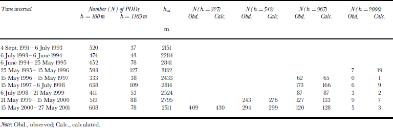
Our calculated estimates of N(h) at AWS sites are in reasonable agreement with the observations, and values of h m in Table 2 are similar to elevations at the inland limit of surface melting, derived from time series of satellite passive-microwave data (personal communication from T. Mote, 2001). Consequently, we used Equation (5) to calculate values of N for each time interval between ATM surveys at any elevation in the basin, from which we inferred corresponding values of (M s + V d) over the same period using Equation (4).We then used the average values of A and (M s + V d) over the entire period, 1991–2001, as A m and (M m + V m) in order to calculate values of A ′ and (M ′ + V ′) for each time interval.
4. Results
Because of excessive noise in the ΔS characteristics, we separated the data into 250 m elevation bands (apart from the lowest 250 m) and solved Equation (3) using average values of ΔS for each of these, assigning an elevation equal to the average elevation of all ΔS measurements within the band. Below 250 m, we used three values of ΔS: one for an elevation band from 110 to 250 m, which refers to the lowest grounded part of the glacier; one derived for the “ice rumples” section; and one derived for the “floating” section. Results are shown in Table 3, as comparisons with the reference year 1997.
Table 3. Measured elevation changes (ΔS) and calculated dynamic thinning (D′ ΔT) at different elevations within the Jakobshavn drainage basin (for various time periods (ΔT ))
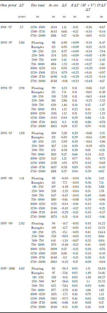
The final column in Table 3 gives estimates of the total dynamic thinning between the ATM observation periods and the 1997 survey. The rate of dynamic thinning (D ′) between consecutive surveys can then be calculated by differencing sequential values of D ′ ΔT, and dividing the difference by the time interval between observations. Results are plotted against elevation in Figure 3 and against time in Figure 4. Here, the elevation is the mean of the average elevations for the two observation periods. It is clear from Figures 3 and 4 that D ′ is negative at most elevations until 1997, indicating that the glacier was dynamically thickening compared to our assumed steady state, with thickening most pronounced at elevations up to about 1000 m. Thickening rates were highest between 1993 and 1995, followed by a substantial reduction until 1997, after which there was a marked transition to large positive values of D ′ (i.e. dynamic thinning). Thinning was initially confined to the lowest 500 m, but progressively migrated inland until, between 1999 and 2001, D ′ was positive at all elevations (Fig. 4).

Fig. 3. Rate of dynamic thinning (D′) plotted against elevation for the periods between ATM surveys, with the envelope of estimated errors shown in the lower panel.

Fig. 4. Rate of dynamic thinning (D′) plotted against time.
Errors in surface-elevation change (ΔS), snow accumulation (A) and surface melting and compaction (M s + V d ) all contribute to errors in the estimates of D ′ plotted in Figures 3 and 4. Of these, errors in ΔS at low elevations are probably the largest, because of large spatial variability in ΔS associated with surface roughness and crevasses and the advection of local topographic features. Although we cannot determine the magnitude of each of these contributing errors, Figure 3 provides an indication of their overall impact on our estimates of D ′. Above 1000 m elevation, most of the pre-1997 estimates fall within about ±0.5 m a−1, suggesting that the overall uncertainty in D ′ at higher elevations is about ±0.5 m a−1. At lower elevations, there is far higher variability in D ′, even before 1997. Here, we would expect errors in ΔS, A and M to be independent from year to year, so the interannual variability before 1997 probably gives an indication of the effect of these errors on D ′. Indeed, this is probably a worst-case error estimate because some of the interannual variability in D ′ may reflect real changes in ice dynamics near the calving front, where rapid changes are more likely. Based on these considerations, error bars in Figure 3 are ±1.5 m a−1 at the lowest elevations, decreasing linearly to ±0.5 m a−1 at 1000 m elevation and above.
5. Discussion
The results shown in Figures 3 and 4 indicate that, before 1997, ice above 1000 m elevation in the Jakobshavn drainage basin was in approximate dynamic balance, with probable thickening at lower elevations at rates that reached maximum values of >1 m a−1 near the ice front. After 1997, there was a major shift to rapid thinning at lower elevations, reaching a maximum near the ice front where dynamic thinning rates progressively increased to >10 m a−1 after 1998. Above about 1000 m elevation, the ice remained approximately in balance, but the thinning zone at lower elevations migrated inland so that, by 1999–2001, it included all elevations up to about 1200 m and perhaps higher. The dynamic thinning rate comprises two components: a change in vertical ice creep ![]() and a change in ice advection (U∂H/∂x). In a glacier basin, such as Jakobshavn Isbræ, advection associated with increased horizontal velocities favors thickening of the glacier by bringing additional thicker ice from upstream. Conversely, a slow-down of the northern branch of Jakobshavn Isbræ would favor thinning along our surveyed profile. However, ATM crossing-point comparisons show thinning over most of the southern branch also, so we discount this possibility. Instead, we propose that thinning by enhanced creep after 1997 predominated over thickening by increased advection within a zone close to the ice front that progressively migrated upstream to reach at least 1200 m elevation (approximately 55 km inland from the glacier calving front) by 1999–2001. 1997 also marked a change to generally warmer summers, with the average annual PDD value for the years 1997–2000 at Egedesminde higher than for any other 4 year period since 1962. However, the longest temperature record in Greenland, from Nuuk on the west coast about 500 km south of Jakobshavn, shows summer temperatures since the mid-1960s were slightly cooler than those between the start of records in 1870 and the late 1920s, and far lower than those between 1930 and the mid-1960s (these records were obtained from the U.S. National Climate Data Center through the Goddard Institute for Space Studies and can be down-linked from http://www.giss.nasa.gov/data/update/gistemp/station_data/).Thus, the sequence of Jakobshavn ice-front retreat between 1880 and 1964, and the more recent dynamic behavior of the glacier, follows the same pattern as the summer temperatures. This suggests quite large and rapid responses of the glacier dynamics to sustained changes in summer temperatures. If so, what are the causes of these responses?
and a change in ice advection (U∂H/∂x). In a glacier basin, such as Jakobshavn Isbræ, advection associated with increased horizontal velocities favors thickening of the glacier by bringing additional thicker ice from upstream. Conversely, a slow-down of the northern branch of Jakobshavn Isbræ would favor thinning along our surveyed profile. However, ATM crossing-point comparisons show thinning over most of the southern branch also, so we discount this possibility. Instead, we propose that thinning by enhanced creep after 1997 predominated over thickening by increased advection within a zone close to the ice front that progressively migrated upstream to reach at least 1200 m elevation (approximately 55 km inland from the glacier calving front) by 1999–2001. 1997 also marked a change to generally warmer summers, with the average annual PDD value for the years 1997–2000 at Egedesminde higher than for any other 4 year period since 1962. However, the longest temperature record in Greenland, from Nuuk on the west coast about 500 km south of Jakobshavn, shows summer temperatures since the mid-1960s were slightly cooler than those between the start of records in 1870 and the late 1920s, and far lower than those between 1930 and the mid-1960s (these records were obtained from the U.S. National Climate Data Center through the Goddard Institute for Space Studies and can be down-linked from http://www.giss.nasa.gov/data/update/gistemp/station_data/).Thus, the sequence of Jakobshavn ice-front retreat between 1880 and 1964, and the more recent dynamic behavior of the glacier, follows the same pattern as the summer temperatures. This suggests quite large and rapid responses of the glacier dynamics to sustained changes in summer temperatures. If so, what are the causes of these responses?
Sustained changes in summer temperatures have an immediate impact on surface melt rates within Jakobshavn’s extensive ablation region and, if ocean waters are also warmer, on basal melt rates from beneath the floating tongue. Surface melt rates may affect glacier dynamics by controlling the flux of meltwater reaching the glacier bed to affect resistance to glacier sliding, and basal melting could influence the buttressing effect on glacier flow of the floating tongue by changing its thickness and the distribution of grounded ice rumples within the floating tongue. Dynamic thinning resulting from these several effects has been described by Reference HughesHughes (1986) as “the Jakobshavns effect’. Reference Echelmeyer and HarrisonEchelmeyer and Harrison (1990) found that surface melt does not affect Jakobshavn Isbræ seasonal velocities, suggesting strong temporal damping of the summer meltwater pulse. However, results from near Swiss Camp (Reference Zwally, Abdalati, Herring, Larson, Saba and SteffenZwally and others2002) show an increase in ice velocities during the very warm summers in the late 1990s, with little or no increase in years with low melt. It is possible that faster parts of the glacier respond differently from the slower ice near Swiss Camp, or there may be a critical level of melt at which flow rates increase.
The effect of dynamic thinning of the glacier will also affect the floating ice tongue as ice flowing across the grounding line becomes progressively thinner, but creep thinning rates for the floating ice should not increase, and the change in surface elevation (ΔS) should be far less than for grounded ice. However, it is clear from Figure 5 that after 1997 the floating ice thinned substantially. Elevation reduction between 1997 and 2001 for the “floating” section (F in Fig. 5) was approximately 35 m, implying a thinning of about 320 m at an average rate of 80 m a−1, assuming the ice was indeed floating. This is far higher than thinning rates of grounded ice immediately upstream, and must have been caused by massive increases in basal melt and/or creep thinning, on the floating ice tongue. Ice freeboard in 1997 was approximately 75 m, so that H was about 690 m. Velocities on the ice tongue were 6–7 km a−1 during the 1980s (Reference Echelmeyer and HarrisonEchelmeyer and Harrison, 1990), with little or no increase towards the ice front, so creep rates then were probably quite small. If this was also the case prior to 1997, the observed drop in surface elevation implies an increase in basal melt rate of up to 80 m a−1 or a creep thinning rate of as much as 0.12 a−1 (∼3.7 × 10⁻⁹ s−1). The Jakobshavn floating ice tongue flow between fjord walls that probably limit lateral creep to quite small values, so the longitudinal and vertical creep rates have approximately the same magnitude, expressed by:
(Reference ThomasThomas,1973), where h is the ice-tongue freeboard and H its thickness, ρ
i is the density of ice, B is the temperature-dependent ice hardness parameter averaged over ice thickness, and F is the “back force”, per unit width of ice tongue, associated with shear past ice margins and over seabed beneath ice rumples, and compression upstream of ice rises. For h = 75 m, H = 690 m and F = 0, this gives B ∼ 1.1 × 10⁵ kPa s1/3, assuming that all of the thinning was caused by creep, and that rapid thinning of the floating-ice tongue after 1997 was caused by a reduction of F to zero. The temperature corresponding to this value of B is approximately −8°C (Reference PatersonPaterson, 1994, p. 97). This may be close to the effective temperature of the floating ice, considering that a thick, basal layer of temperate ice has been postulated for Jakobshavn Isbræ (Reference Iken, Echelmeyer, Harrison and FunkIken and others1993), much of the rest of the ice column could be warmed by refreezing of abundant meltwater flowing into crevasses and moulins below the equilibrium line at about 1100 m elevation, and the colder, near-surface ice is weakened by deep crevasses. However, as the floating ice became thinner, h and H in Equation (6) would become smaller, yielding progressively smaller values for the creep rate ![]() Moreover, the back force F is unlikely to have decreased to zero. Consequently, increased basal melt was almost certainly responsible for much of the thinning since 1997.
Moreover, the back force F is unlikely to have decreased to zero. Consequently, increased basal melt was almost certainly responsible for much of the thinning since 1997.

Fig. 5. A sequence of elevation profiles along the main line, extending from the ice front to 600 m elevation. The probable grounding-line location (G) is based on transition from higher-elevation, rugged topography to lower, near-horizontal surfaces, and possible locally grounded ice rumples (A–C) are identified where “hills”persist from year to year.The two sections for which we inferred elevation changes are also shown: one on near-hori-zontal and probably floating ice (F), and one on the most seaward of the ice rumples (R). The ice rumples discussed by Reference Echelmeyer, Clarke and HarrisonEchelmeyer and others, (1991) as possibly having a stabilizing influence on the ice front are at D on the Landsat image from 20 May 2001 showing the flight track of the main line. The horizontal scales for the profiles and the Landsat images are the same.
Melting from beneath ice shelves and floating ice tongues is extremely sensitive to ocean conditions, with melting rates ranging from a few cm a−1 to tens of m a−1 (Reference Jacobs, Hellmer, Doake, Jenkins and FrolichJacobs and others1992; Reference RignotRignot, 1996; Reference Jenkins, Vaughan, Jacobs, Hellmer and KeysJenkins and others1997; Reference Rignot and JacobsRignot and Jacobs, 2002). There have been a number of observations showing quite large temperature and salinity changes recently in both the North Atlantic and the Arctic (Reference Steele and BoydSteele and Boyd, 1998; Reference DicksonDickson and others2000; Reference Morison, Aagaard and SteeleMorison and others2000; Reference SerrezeSerreze and others2000), and it is possible that increased basal melting from floating ice tongues could result from these changes. Figure 6 shows a time series of PDDs at Egedesminde since 1949, and one of sea-surface temperatures (SSTs) for the same period, averaged over the four warmest months (July–October) for the North Atlantic and Davis Strait at 50–65° N, 45–65° W (personal communication from S. Hakkinen, 2002). These SSTs are averaged over 2.5° × 2.5° ice-free grid squares during 1948–2001, and are the same as those used in the U.S. National Centers for Environmental Prediction/U.S. National Center for Atmospheric Research (NCEP/NCAR) re-analysis (http://www.cdc.noaa.gov/reanalysis.html).

Fig. 6 Time series of Egedesminde PDDs since 1949, and of SSTaveraged for the four warmest months (July–October) over the North Atlantic and Davis Strait at 50–65° N, 45–65° W (personal communication from S. Hakkinen, 2002).
The warming in the latter half of the 1990s extends to the deeper ocean also, as shown by the TOPEX altimeter time series from the same area (personal communication from S. Hakkinen, 2002), and can be explained by decreased meridional overturning during a strongly negative NAO, as simulated by a numerical model (Reference HäkkinenHakkinen, 1999, Reference Häkkinen2001). The sea-surface height (SSH) measured by TOPEX contains signals both from vertical stratification changes and from barotropic wind-driven effects. Although the latter contribution increases towards high latitudes, the positive trend of both SSTand SSH suggests that warming extended deeper into the water column below the thin surface layer. This is supported by temperature profiles measured in the West Greenland Current at about 60.5° N, showing a steady increase of the maximum temperature in the current from 3.5°C in 1994 to 4.8°C in 1999, and temperature profiles from 20–500 m depth at three stations over the West Greenland Slope near 60° N showing an increase in the average temperature from 3.7°C for 1990–95 to 4.1°C for 1996–2000 (personal communication from J. Lazier, 2002). The SSTs show a similar pattern to the Egedesminde PDD values, suggesting that summer temperatures along the west coast of Greenland are driven by nearby ocean conditions. Both show recent values higher than at any time since the 1960s, with the intervening period coinciding with a more-or-less stable location for the Jakobshavn ice front.
6. Conclusions
Recent substantial thinning of the grounded part of Jakobshavn Isbræ results from dynamic processes rather than increased melting or reduced snowfall. It could be partly explained by glacier acceleration induced by increased basal lubrication as excess surface meltwater drains to the glacier bed. However, highest thinning rates are inferred for the floating ice tongue, implying increased basal melt rates and/or increased longitudinal creep rates, with the strong probability that both mechanisms are required to explain the extremely high thinning rates. Increased creep rates would result from a reduction in the back force acting on the floating ice tongue.The back force is probablycaused by resistance from shear past the fjord sides, iceberg fragments choking the fjord, and grounded areas such as ice rumples A–D identified in Figure 5. Ice rumples A–C started to thin after 1997, so a large reduction in F is most readily explained by substantial weakening of these and the larger ice rumples (D) to the south of our survey line, as surrounding areas of the floating tongue thinned sufficiently for the ice to float free. This thinning could have been initiated by an increase in basal melt rates on the floating ice tongue as ocean temperatures began to increase after the warm summer of 1995, when dynamic thickening rates on the floating tongue began to decrease.
The ice front advanced about 3 km between 1991 and 1997, followed by a 4 km retreat, and an apparent 2 km advance between 1999 and 2001. However, the floating ice tongue in May 2001 was deeply fractured within 6 km of the ice front, and a Landsat image from 7 July 2001 showed that most of this ice had calved, with the ice front approximately at the location of ice rumple A in Figure 5. This ice rumple appears to have become ungrounded by May 2001 following very rapid thinning between 1999 and 2001 (Fig. 4), and the other ice rumples (B and C in Fig. 5) also thinned appreciably after 1999. We should note that most of our measurements were made over the slower, northern branch of the glacier and the region of slow-moving ice between the northern and southern branches, suggesting the possibility that observed thinning is simply indicative of a slow-down of the northern branch. However, the thinning zone extends into the region of slower-moving ice, and many spot measurements over the rest of the glacier basin also show appreciable thinning. Consequently, we believe that our observations are indicative of conditions over the entire glacier. Following our most recent survey, summer temperatures were also high for 2001, with the annual PDD at Egedesminde higher than for any year since 1960 (Fig. 6), and a strong probability of continued thinning and possible ungrounding of the remaining ice rumples. This could lead to a retreat of the calving ice front to a new position at the grounding line (G in Fig. 5), where the ice sharply rises inland. This position is close to large icefalls, presumably overlying shallow bedrock, that separate the main, southern branch of the glacier from its slower, northern branch. The two branches would then calve directly into the ocean, and would probably continue to thin further inland towards a new configuration consistent with the loss of buttressing by the floating tongue. Since this paper was first submitted for publication, in March 2002, a moderate-resolution imaging spectrometer (MODIS) image from July 2002 (http://modis.gsfc.nasa.gov/galleryDB_DATE=2002-07-20) showed that the ice front had retreated about 3 km from its position in Figure 5.
Acknowledgements
This work was supported by the NASA Cryospheric Sciences Program and ICESat Project. We thank all who helped to make the various measurements used in our analysis, and we are particularly grateful to S. Hakkinen (NASA Goddard Space Flight Center, Greenbelt, MD), J. Lazier (Bedford Institute of Oceanography, Dartmouth, Nova Scotia, Canada) and T. Mote (University of Georgia, Athens, GA) for providing us with unpublished information from their own research. We also thank J. Meyssonnier (Scientific Editor) and two anonymous referees for suggestions that improved and clarified the text.


