


Introduction
Apowder-snow avalanche is a dense cloud of suspended snow particles moving down a steep slope. These flows can reach front velocities uf of 100 ms–1, and heights h of the order of 100 m.Measurements by intrusive probes are therefore very hazardous. In addition, powder-snow avalanches are rare events. Techniques such as georeferenced photography and radarnow in use provide extremely valuable information concerning the avalanche dimensions, their shape and front velocities, as well as velocities behind the front (Reference Dufour, Gruber and AmmannDufour and others, 2001a, Reference Dufour, Gruber, Bartelt and Ammannb). However, density or snow-concentration measurements still rely on intrusive probes and are relatively uncertain.
In parallel, laboratory experiments, simulating avalanches, were developed which provided useful information about the dynamics of these flows and the dependency of avalanche velocity and shape on slope angle. A review of laboratory experiments and the related theoretical models can be found in Reference HopfingerHopfinger (1983) and Reference HutterHutter (1996). The theoretical models show that entrainment of snow from the snow cover is an important aspect of avalanche motion (Reference Hopfinger and Tochon-DanguyHopfinger and Tochon-Danguy, 1977; Reference Fukushima and ParkerFukushima and Parker, 1990; Reference Rastello and HopfingerRastello and Hopfinger, 2004). Generally, laboratory experiments are, unfortunately, limited to Boussinesq fluids of Boussinesq number (ϱ2 - ϱ1)/ϱ2 ≪ 1. The principal similarity parameter is the densimetric Froude number provided the Reynolds number is sufficiently large for the flow to be fully turbulent (in free shear flows, a continuous energy spectrum with a k-5/3 spectral slope emerges when the flow Reynolds number is greater than 3 × 10⁴).
Commercial avalanche codes use depth-averaged models and in some cases turbulence k - ε models for the powder cloud. Often these models are combined with a dense flow layer below the powder cloud and a transition layer in between (see, e.g., Reference Naaim and GürerNaaim and Gürer, 1998).
Progress in understanding the flow structure requires more refined experiments (field studies and laboratory experiments). Direct numerical simulations (DNS) and large eddy simulations (LES) are alternative approaches. These give access to all the flow quantities desired and would be of particular interest for the study of the interaction of an avalanche with structures, for instance. Unfortunately, the complex structure of avalanches makes such numerical simulations difficult. For this reason, only Boussinesq gravity currents on a horizontal boundary have been simulated at present (Reference Necker, Härtel, Kleiser and MeiburgNecker and others, 2002). Here we present the first DNS of dense-cloud motion on slopes. These simulations are, at present, two-dimensional and for ![]() the relevance of two-dimensional simulations, which allow high Reynolds numbers to be reached, is supported by the dynamics of avalanches discussed below. Before refining the simulations by going to a three-dimensional code, it is of interest to study such first-order effects as snow entrainment and large (ϱ2 - ϱ1)/ϱ2. Ultimately, DNS and LES can serve as benchmark tests for averaged models used in practice.
the relevance of two-dimensional simulations, which allow high Reynolds numbers to be reached, is supported by the dynamics of avalanches discussed below. Before refining the simulations by going to a three-dimensional code, it is of interest to study such first-order effects as snow entrainment and large (ϱ2 - ϱ1)/ϱ2. Ultimately, DNS and LES can serve as benchmark tests for averaged models used in practice.
Characteristics and Dynamics of Powder-Snow Avalance Flow
The density of avalanches ranges from about 20 kgm–3 near the start to about 2 kgm–3 at the end. The settling velocity and volume concentration of the snow particles are small, so that the energy required to keep the particles insuspensionisa small fraction of the turbulent kinetic energy. Furthermore, the particle time-scale τp = ws/g, wherews is the fall velocity and g the gravitational acceleration) is about one-tenthof the flow time-scale h/uf. Hence, the particles closely follow the local velocity of the cloud, whichallows, as a first approximation, treatment of the avalanche as avariable density fluid.
Laboratory experiments with dense clouds carried out by Reference Beghin, Hopfinger and BritterBeghin and others (1981), Reference Hermann, Hermann and HutterHermann and others (1987) and more recently by Reference RastelloRastello (2002) showed that the main features of avalanche flow can be reproduced with single-phase, variable-density flows, and demonstrated two essential features of these flows:
The force balance governing the flow is between the driving buoyancy force and the entrainment of ambient fluid (air in the case of avalanches). As ambient fluid is entrained, it has to be accelerated, and this momentum transfer results in an effective drag, which has an effect of much larger magnitude than ground friction. There is practically no flow separation, so the form drag is negligible. The interfacial friction is included in the entrainment.
The entrainment of ambient fluid is caused by the overturning motion of the large structures of the flow.
The generation of the large structures responsible for the entrainment of ambient fluid is essentially a two-dimensional mechanism. The smaller-scale three-dimensional turbulence of the flow is superimposed on the larger features. The effect of these three-dimensional structures on the air entrainment can be neglected in a first-order approach. Indeed, Reference NormandNormand (1990) demonstrated by comparison with numerous laboratory experiments that two-dimensional simulations of a mixing layer reproduce well the actual spreading rate of the flow. Therefore, we can expect that two-dimensional DNS can reproduce fairly well the essential physics and dynamics of laboratory clouds and also powder-snow avalanches. This allows us to focus on solving accurately this simplified problem rather than dealing with the complexity of three-dimensional simulations.
Within this frame, we shall proceed first with validating our assumptions by comparing the simulations with laboratory clouds, for which we have accurate quantitative results. Then the simulations are extended to avalanches.
The comparison with laboratory experiments allows two further approximations which will provisionally be used in our simulations: (i) The ratio of the density of the aerosol to the ambient fluid density is close to one (whereas it is closer to 10 for avalanches), i.e. we can use the Boussinesq approximation; (ii) the Reynolds number is of order 104, rather than 109 for avalanches. It should be noted that the actual value of the Reynolds number is not of primary importance (because the dynamics is controlled by the large-scale features and depends only weakly on the smaller scales) as long as it is sufficiently large (Re≥104).
Small-scale laboratory dense clouds are limiting cases of avalanches, as was clearly shown by Reference RastelloRastello (2002) by comparing laboratory results with observations by Reference Dufour, Gruber and AmmannDufour and others (2001a).
Variable-Density Flow Equations
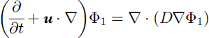
Let us consider a fluid which is a mixture of two miscible species with different properties, and define a volume fraction of each of them, Φ1 and Φ2, in a domain Ω, such that Φ1 + Φ2 = 1. Inourcase, the species are the initial dense fluid (snowaerosol) and the ambient fluid (air).
Following Reference Joseph and RenardyJoseph and Renardy (1993), we assume that the diffusion within the mixture is governed by Fick’s law, and assuming Boussinesq conditions we obtain the system:
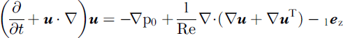
which is non-dimensionalized by the velocity scale ![]() which is the free-fall, terminal velocity of the fluid in the light one. The Reynolds number is defined as
which is the free-fall, terminal velocity of the fluid in the light one. The Reynolds number is defined as ![]() The characteristic lengthLis chosenas the length ℓ0 of the heavy fluid volume initially released (note that often the characteristic length scale is taken as
The characteristic lengthLis chosenas the length ℓ0 of the heavy fluid volume initially released (note that often the characteristic length scale is taken as ![]() (see Fig. 1). All results are presented in this non-dimensional form, i.e. velocity is normalized by U, the distance
(see Fig. 1). All results are presented in this non-dimensional form, i.e. velocity is normalized by U, the distance ![]() and cloud dimensions by L, and the time byL/U. We use non-slip conditions on the boundary; the domain is chosen large enough so that its finiteness does not affect the solution.
and cloud dimensions by L, and the time byL/U. We use non-slip conditions on the boundary; the domain is chosen large enough so that its finiteness does not affect the solution.

Fig. 1. Definition sketch. The star denotes dimensional counterparts of quantities otherwise used in non-dimensional form.
Numerical Method
Time discretization
Inorder to avoid the numerical instabilities that usually originate from half-implicit schemes with large time-steps, we use the characteristics method proposed by Reference PironneauPironneau (1989), i.e. wediscretize directly the material derivative[(∂/∂t) + u • ▽] along the trajectory of a fictious particle X moving with the velocity u(X). It is thus possible to write an implicit Euler scheme for Equations (1a) and (1b–1c), respectively.
Space discretization
We use the Taylor–Hood finite element (Reference Hood and TaylorHood and Taylor, 1973), which is a continuous piecewise quadratic approximationof u and Φ, and a continuous piecewise linear approximationof p. Equation (1c) is enforced up to machine precision by an augmented Lagrangian iterative algorithm (Reference Fortin and GlowinskiFortin and Glowinski, 1983) over Equations (1b–1c).
The flow being of “impulse” type, with locally high gradients in the shear and boundary layers, there is an obvious benefit in locally refining the mesh as shown in Figure 2 (Reference Saramito and RoquetSaramito and Roquet, 2000). We refine according to the Hessians of both the local energy dissipation and the phase volume-fraction in order to have the boundary layers and high-shear regions refined as well as the interface. It requires approximately 6 min to run a one-time-step iteration of four mesh adaptations on an Intel/Linux 1 GHz personal computer. A reasonable time-step is 0.05 in non-dimensional units, that is approximately 0.25 s for a large avalanche.
Fig. 2. Detail of the adaptive mesh in Figure 5. Note the refinement in the boundary layer close to the ground and along the density map isolines (shown as background).
Results
Validation
Our validation in this paper relies on the spatial growth and front velocity of the aerosol cloud as it moves down the slope. For a fine enough mesh, the features of the solution become mesh-invariant, which means that the numerical convergence is assured. It is shown in Figure 3 that the calculated front velocity is found similar to the experimental front velocity. In Figure 4 we compare the calculated evolution of cloud height and length with laws experimentally established by Reference Beghin, Hopfinger and BritterBeghin andothers (1981) and by Reference RastelloRastello (2002). It is seen that the evolutions are similar.
Fig. 3. Comparison of the non-dimensional front velocity υs non-dimensional front position in simulations and in experimental clouds of Reference RastelloRastello (2002).
Fig. 4. Comparison of the spatial growh of cloud length and height in simulations on a slope of angle θ = 32°.
Flow structure
As noted both in realavalanches and in laboratory clouds, the flow consists of two well-identified parts, namely the head, which reaches large heights and develops shear-layer instabilities, and the tail (awake), which flows more slowly, close to the ground. The numerical simulations display an even stronger separation between these two parts.
An essential feature is the ambient fluid entrainment, which causes the main drag. It is strongest at the rear of the head in experiments (Reference Hopfinger and Tochon-DanguyHopfinger and Tochon-Danguy, 1977; Reference Rastello and HopfingerRastello, 2002) and is also clearly so in our numerical simulations (Fig. 5). The shear flow instability is also seen in the time sequence (Fig. 6) and was found in both of the above-cited experiments. Two other vortices rotating opposite to the shear-layer eddies are exhibited, one of them having been noticed by Reference Rastello and HopfingerRastello (2002) in experiments. Moreover, it was noted in these experiments that heavy fluid from the forepart of the head was periodically rejected into the large vortex at the rear, a process also exhibited by the numerical simulations.
Fig. 5. Qualitative comparison between (a) laboratory cloud of Reference RastelloRastello (2002) and (b) numerical simulation of a Boussinesq cloud at time t = 12.8 on a 32° slope, with Re = 104. Superimposed in black are the large eddy motions and in white the air-entrainment process. Themesh of the front part is shown in Figure 2.
Fig. 6. A time sequence of density maps in numerical simulations, for t = 11.8; t = 12.3; t = 12.8 and t = 13.3. Conditions are the same as in Figure 5. Note that the maximum of Φ1 diluted down from1 to 0.95.
Kinetic energy and dynamic pressure
Awell-known manifestation of avalanches is their destructive power, which is observed to be much larger in practice than estimated from the average density and front velocity (Reference Berthet-RambaudBerthet-Rambaud, 2001). One possible explanation is that the dynamic pressure inside the avalanche is locally much larger. The dynamic pressure is ![]() and, the ambient fluid density
and, the ambient fluid density ![]() being small in an avalanche, it is essentially equal to
being small in an avalanche, it is essentially equal to ![]() We compare it to the front average stagnation pressure, that is
We compare it to the front average stagnation pressure, that is ![]() where
where ![]() (respectively
(respectively ![]() is the average of the density (respectively of
is the average of the density (respectively of ![]() over the head. It is shown in Figure 7 that very high ratios (around 7) are reached locally where there are high velocities in dense areas. The existence of such large dynamic pressures inside the avalanche behind the front was suggested by Reference HopfingerHopfinger (1983) and has also been noted by other authors (personal communication from D. Issler, 2003).
over the head. It is shown in Figure 7 that very high ratios (around 7) are reached locally where there are high velocities in dense areas. The existence of such large dynamic pressures inside the avalanche behind the front was suggested by Reference HopfingerHopfinger (1983) and has also been noted by other authors (personal communication from D. Issler, 2003).
Fig. 7. Ratio of maximum over z of excess dynamic pressure ![]() to front average stagnation pressure at t = 12.8. The plus signs denote the loci of the maxima; isolines Φ = 0.08 and Φ = 0.35 are also shown.
to front average stagnation pressure at t = 12.8. The plus signs denote the loci of the maxima; isolines Φ = 0.08 and Φ = 0.35 are also shown.
Discussion
The direct numerical simulations presented in this paper show that two-dimensional simulations reproduce the essential features of gravity currents, including avalanches. The assumption of two-dimensionality seems at first sight very stringent because the visual appearance of an avalanche flow in two dimensions is quite different; the large vortices seen in avalanches as well as in laboratory clouds appear fully three-dimensional. Their strength, however, is determined by the two-dimensional mean shear, which justifies two-dimensional simulations as a good first approach. Indeed, the corresponding numerical results compare well with laboratory results. This is because the force balance is accounted for by the gravitational force which drives the avalanche, and by entrainment of ambient fluid, which is the principal retarding force and is essentially a two-dimensional process. Since laboratory experiments with Boussinesq fluids are well reproduced in our simulations and since these laboratory avalanches have the same three-dimensional structures and involve the same governing mechanisms as the real avalanches, wecanhopetosimulateavalanchesbytaking into accountthelargerdensitydifference.Thisrequirestheextension of the model and code to non-Boussinesq flows, which was done recently by Reference Étienne, Hopfinger and SaramitoÉtienne and others (2004).

