


Introduction
The chemistry within firn and ice cores, such as those collected by the International Trans-Antarctic Scientific Expedition (ITASE) (Reference MayewskiMayewski, 1996; Reference MayewskiMayewski and others, 2006), contains information about the soluble, insoluble and gaseous components of the atmosphere, as well as indicators of temperature, precipitation, atmospheric circulation, sea-ice extent and volcanic activity (Reference Legrand and MayewskiLegrand and Mayewski, 1997). The microstructure of firn and ice cores, such as the size, morphology and orientation of grains, has also been shown to be indicative of the physical, mechanical and chemical characteristics of the ice sheet from which they were extracted (e.g. Reference Alley, Perepezko and BentleyAlley and others, 1986, Reference Alley, Gow, Johnsen, Kipfstuhl, Meese and Thorsteinsson1995a; Reference Thorsteinsson, Kipfstuhl, Eicken, Johnsen and FuhrerThorsteinsson and others, 1995; Reference Alley and WoodsAlley and Woods, 1996; Reference Cuffey, Thorsteinsson and WaddingtonCuffey and others, 2000). Temperature, ice flow and impurity content can all be inferred using these properties, so accurate physical properties measurements are important to our understanding of ice cores as proxies for climate. More recently, much attention has been given to characterizing the microstructural location and composition of impurities in ice cores. Knowledge of these characteristics will increase our understanding of grain growth, deformation, diffusion and electrical conduction, as well as the likelihood of post-depositional interactions that may affect the reliability of climate proxies (Reference Kreutz, Mayewski, Whitlow and TwicklerKreutz and others, 1998). While much of this attention has focused on refining the methodology (Reference Cullen and BakerCullen and Baker, 2001; Reference Barnes, Mulvaney, Wolff and RobinsonBarnes and others, 2002b, Reference Barnes, Wolff, Mallard and Mader2003; Reference Baker and CullenBaker and Cullen, 2003; Reference Baker, Iliescu, Obbard, Chang, Bostick and DaghlianBaker and others, 2005, Reference Baker, Obbard, Iliescu and Meese2007), defining and describing impurity types (Reference Barnes, Mulvaney, Robinson and WolffBarnes and others, 2002a; Reference Obbard, Iliescu, Cullen and BakerObbard and others, 2003; Reference Barnes and WolffBarnes and Wolff, 2004) and studying crystallographic orientation (Reference Baker, Iliescu, Obbard, Chang, Bostick and DaghlianBaker and others 2005; Reference Obbard, Baker and IliescuObbard and others 2006; Reference Obbard and BakerObbard and Baker, 2007), only limited work has been done to directly relate the morphology and micro-structural location of impurities to the physical properties they are believed to affect (Reference Barnes, Mulvaney, Robinson and WolffBarnes and others, 2002a; Reference Iliescu and BakerIliescu and Baker, 2008). Scanning electron microscopy (SEM) is used here to examine those relationships spatially and temporally in a suite of samples collected by the US ITASE team.
Methods
Sample collection, storage and preparation
Eight firn and ice cores were collected during the 2006 and 2007 US ITASE traverses (Fig. 1) using the methodology described by Reference SteigSteig and others (2005). Four of the eight cores (06-1, 06-2, 06-3 and 07-4) were drilled to ∼100 m; the other four were drilled to ∼40–50 m depth and were excluded from this study. Approximately 0.75 in (19 mm) thick vertical sections were cut from the selected 3 in (∼76 mm) cores. These sections were sealed in plastic and maintained in a −20°C freezer. On the day of analysis, horizontal subsamples (the surface analyzed is perpendicular to the core axis) were cut from these sections, and the face to be analyzed was shaved with a razor blade at −20°C under a High Efficiency Particle Air (HEPA)-filtered laminar flow hood following standard clean-room practices. The final specimens were flat, smooth, free of scratches and had maximum dimensions of 0.5 cm × 1 cm × 3 cm (Reference Cullen and BakerCullen and Baker, 2001). Horizontal sections were taken every 10 m from all four cores (Table 1). Specimens were placed in a spring-loaded copper sample holder, covered with a plastic cap to prevent contamination and the formation of frost on the surface and transported to the microscopy laboratory in a liquid nitrogen atmosphere.

Fig. 1. Map of core locations. 06-1, 06-2, 06-3 and 07-4 (black circle with ring) are analyzed in this study. 02-5 and 03-1 (black circle with white dot and ring) are used for comparison of EDS and IC-PMS data (created by D. Dixon using RADARSAT-1 Anatarctic Mapping Project digital elevation model (RAMP DEM); H. Liu and others, nsidc.org/data/nsidc-0082.html).
Table 1. Physical properties data for the firn cores used in this study. Grain size and density increase with depth, while porosity and internal surface volume (S V) decrease with depth

Analytical techniques
Scanning electron microscopy
Samples were maintained at −110 ± 5°C in the vacuum chamber of an FEI XL30 field emission gun SEM during data collection. The SEM was operated at 15 kV with a beam current of 0.15 nA and a spot size of 3 μm. During the collection of electron backscatter diffraction patterns (EBSPs) the spot size was increased to 5 μm (Reference Baker, Obbard, Iliescu and MeeseBaker and others, 2007). For each sample a series of slightly overlapping SEM images was collected. These images were digitally stitched together to form a mosaic of the horizontal surface of each sample. These mosaics were used to calculate grain size and porosity. Grain sizes were determined by tracing grain boundaries on SEM images using the drawing tool in Image-Pro Plus 5.0© and then utilizing a pixel counter to determine area (Reference Spaulding, Meese, Baker, Mayewski and HamiltonSpaulding and others, 2010). Porosity was calculated as percent areal porosity by dividing the area of pores by the area of the field of view. The repeatability of porosity measurements (±1.2%) was determined by repeating the porosity determination of ten samples from different depths.
A light-element Si (Li) detector coupled to the SEM was used to collect energy-dispersive X-ray spectra (EDS) for identification of the elements present in the observed impurities. The ‘concentration’ is reported as the number of X-ray counts detected. The counts cannot be directly converted into a ‘microgram per liter’ type concentration for a number of reasons. Most of the impurities found in firn and ice are light elements, which produce a small number of low-energy photons that are readily absorbed by the surrounding ice. The decreased production and low energy of the photons result in a low signal-to-noise ratio, which reduces the accuracy of the EDS system. Additionally, the strength of the X-ray current is dependent upon both the size of the impurity analyzed (larger impurities offer a larger interaction volume) and the concentration of chemicals in the impurity. For these reasons, EDS analysis of impurities is considered qualitative, rather than quantitative (Reference GoldsteinGoldstein and others, 1992). EDS were collected from triple junctions, filaments, grain boundary ridges, grain boundary grooves and crystal facets from at least three distinct locations per sample. Background spectra were also taken from areas presumed to be pure ice for purposes of comparison.
EBSPs were obtained for each core at ∼90 m depth using an HKL, Inc. Channel 5 Orientation Imaging System (Reference Day, Trimby, Mehnert and NeumannDay and others, 2004). Due to the size restrictions of the sample holder and the grain size at these depths, more than one ice sample was required to obtain enough patterns to produce statistically significant data. Additionally, because EBSPs in ice can be difficult to index, not all patterns collected are usable. In this study, at least 60 patterns from each sample were of a high enough quality to index. EBSPs, such as those shown in Figure 2, were indexed to produce pole figures for both the a-axes and c-axes using the HKL (CHANNEL 5) pole-figure and inverse pole-figure software package Mambo©. Imaging was performed using a forward-scatter electron detector, and EBSPs were obtained by stopping the beam at a point of interest. Patterns were produced by backscattered electrons collected on a phosphor screen and recorded using a charge-coupled device (CCD) camera. The sample was held by a copper sample holder pre-tilted to 10°, and the stage was tilted an additional 60° to maximize backscattering yield.

Fig. 2. Electron backscatter diffraction pattern from ice with its corresponding crystal orientation.
Experimental Results
Stratigraphy
Stratigraphic analysis was conducted both in the field and in the laboratory. Each section of core was placed on a light table, and the locations of coarse (summer) layers, fine (winter) layers, ice layers, wind crusts and other pertinent data were recorded at the millimeter scale.
Physical properties
Grain size
As expected, grain size in all cores showed a linear increase with depth (Fig. 3) (Reference Stephenson and OuraStephenson, 1967; Reference GowGow, 1969), driven by the reduction in free energy associated with a decrease in grain boundary area. The four cores in this study also exhibit a decrease in grain size with distance from the coast, i.e. core 06-1 located at Taylor Dome (near the coast) has the largest grain size, whereas core 07-4 located at Titan Dome (near South Pole) has the smallest grain size. The change in grain size is attributable to the decrease in mean annual temperature on moving inland (J. Bohlander and T. Scambos, http://nsidc.org/data/docs/agdc/thermap/documentation.html).

Fig. 3. Physical properties data for the four cores used in this study. Grain size (a) and density (d) increase with increasing depth, while porosity (b) and internal surface volume S V (c) decrease with increasing depth. 06-1 has the highest porosity and S V and the lowest density and grain size. 07-4 has the opposite pattern, primarily as a result of the much lower mean annual temperature at this site.
Porosity
Core 06-2 has the lowest average porosity, with cores 06-1 and 06-3 being approximately equivalent. However, 06-1 is less porous at all depths except 30 and 40 m. Visual stratigraphy indicates that these samples were taken from a coarse layer, whereas those from equivalent depths in cores 06-2 and 06-3 were taken from a fine layer, indicating differences in seasonality. Samples were taken from the bottom of each core section without regard for seasonality; if the samples from core 06-1 had been taken from a fine layer, it would likely have the lowest average porosity, in accordance with having the highest overall grain size. Core 07-4 has the highest overall porosity as determined using SEM images, although it may not be significantly different from cores 06-2 or 06-3. The porosity values measured from core 07-4 were erratic and did not exhibit the typical trend of decreasing with depth. A correlation coefficient, r, of 0.72 was found for core 07-4 between porosity and depth by forcing the intercept of the trend line to zero. In order for the correlation to be significant at the 95% level, r (with nine degrees of freedom) must be at least 0.735. All other cores had an r for porosity versus depth of >0.88, which was statistically significant. Ground-penetrating radar (GPR) profiles indicate that coarse-grained hoar layers are thicker and more frequent at site 07-4 than at any of the 06 sites (personal communication from S.A. Arcone, 2008). Visual stratigraphy shows a similar trend, a greater number of thick coarse-grained hoar layers than of thinner fine-grained layers. At all other sites, the number of coarse and fine layers is similar and the fine layers tend to be thicker. The increased chance of sampling an irregular hoar layer likely contributes to the erratic porosity measurements.
Internal surface volume per area
The internal surface volume per unit area was calculated as
where L A is the length of the internal surface lines per unit area as determined by dividing the length of the projected surface around pores by the bounding area of those pores. S V is a measure of the complexity or tortuosity of the pores. Core 07-4 has the highest overall complexity, while core 06-1 has the lowest. In each core, S V increases between 10 and 40–60 m and decreases between 40–60 and 100 m. Reference Baker, Obbard, Iliescu and MeeseBaker and others (2007) used samples with a depth range of 10–40 m in US ITASE cores 02-SP and 02-5 and also found that S V increased with depth. Because S V depends on the length of pore outlines, Reference Baker, Obbard, Iliescu and MeeseBaker and others (2007) hypothesized that the increase to 40–60 m was a result of increasing convolution of pore outlines as the grains were flattened with increasing overburden. The S V values in this study and in Reference Baker, Obbard, Iliescu and MeeseBaker and others (2007) can be explained by assuming that S V is initially low when each grain is an island and then increases as the grains merge and their outlines become more complex to 40–60 m. Once the maximum possible number of contacts between grains has been made, the complexity of the outline no longer changes. Thus, below this depth, continued overburden pressure causes a decrease in pore size, pore outline length and consequently S V. This explanation and the trends in S V agree well with established models of firn densification, which divide the process into three stages. In the first stage, individual grains or small groups of grains are distinguishable within the pores, in the intermediate stage the interconnection of pores is decreased as the contact area between grains reaches a maximum and in the final stage closed-off spherical pores are established (Reference Anderson, Benson and KingeryAnderson and Benson, 1963; Reference Maeno and EbinumaMaeno and Ebinuma, 1983; Reference AlleyAlley, 1987; Reference Ebinuma and MaenoEbinuma and Maeno, 1987; Reference WilkinsonWilkinson, 1988; Reference Arnaud, Gay, Barnola and DuvalArnaud and others 1998, Reference Arnaud, Barnola, Duval and Hondoh2000; Reference Freitag, Wilhelms and KipfstuhlFreitag and others 2004).
Density
Bulk density (ρ) measurements were performed for each core section immediately after retrieval in the field. These measurements revealed that in addition to having the lowest porosity value and the highest degree of anisotropy of pore space, core 06-1 had the highest rate of densification of the four cores (0.0056 kg m−4, i.e. kg m−3 per meter of ice in each core section). Core 07-4 had the lowest rate of densification, although the difference in the rates of densification between 06-2 (0.0037 kg m−4), 06-3 (0.0039 kg m−4) and 07-4 (0.0036 kg m−4) were very small and likely not statistically significant.
Crystallographic orientation
The {0001} and {1120} pole figures produced for each core at ∼90 m are shown in Figure 4. The random distribution of the points in the scatter plots suggests that the grains from all four cores do not have a strongly preferred orientation. The strength of the c-axis fabric was tested using the method of Reference KambKamb (1959), in which a coefficient f is calculated by dividing the number of c-axes, NA , in an area of the projection, A, by the standard deviation, σ, of the number of axes expected from a random distribution. Both A and σ are determined by a statistical relationship from the number of data points evaluated, N SAMP, such that when N SAMP increases, A decreases and σ increases. A value of f < 3 is expected when there is no preferred orientation. Statistically significant preferred orientations indicate that the density of points within A could not have resulted from the random sampling of a population with no preferred orientation and are described by f ≥ 6. Strongly preferred orientations are described by much higher numbers: for example, Reference Hooke and HudlestonHooke and Hudleston (1980) report a strength of 31 for a single-maximum fabric from 156 m depth in Barnes Ice Cap, Canada. All the fabrics analyzed in this study were shown to be statistically significant (Table 2).

Fig. 4. {0001} and {1120} pole figures for samples from ∼90 m depth. Statistically significant preferred orientations are found in all four samples. N indicates the number of grains examined in each core.
Table 2. Determination of the strength of the c-axis fabric using Reference KambKamb (1959). Variables are outlined in the text
Chemical properties
Elemental chemistry
In order to determine whether the elemental chemistry or the distribution of impurities changed with depth, samples from approximately 30, 60 and 90 m in each core were analyzed using EDS. Figure 5 shows the average intensity in counts s−1 of the eight most common elements at each depth in each core and allows inter-site comparison. Although depth was used to identify each sample, the seasonality and age of the stratigraphic layer is more important to the comparison of chemistry than depth alone. Figure 6 shows the average frequency with which each element occurred in either winter or summer, as determined by visual stratigraphy, and allows a comparison of seasonal influences. It may be assumed that an element occurring with greater frequency contributes more significantly to the aerosol/dust loading at the time of deposition.

Fig. 5. The average intensity of the eight most common elements at (a) 30 m, (b) 60 m and (c) 90 m depth. Note that in most cases intensity (concentration) is greatest at 06-1 and lowest at 07-4.

Fig. 6. Frequency of occurrence of the eight most common elements in winter and summer layers as determined by visual stratigraphy. Frequency is calculated by dividing the number of times that element is seen by the number of spectra from that season containing chemistry beyond background levels.
Analytical Results
Elemental factor analysis
Factor analysis, a type of multivariate statistical analysis (Reference FitchFitch, 2007), was used to examine the elemental associations in each of the four cores for which chemical data were collected. Factor analysis attempts to explain the correlation between a large number of variables in terms of a small number of underlying factors (Reference Mardia, Kent and BibblyMardia and others, 1979). Those factors are determined through the extraction of eigenvalues from the data correlation matrix. Factors with eigenvalues greater than 1 represent statistically significant groups of variables (Reference KaiserKaiser, 1960) and are retained. The factor with the highest eigenvalue, F1, explains the highest percent of the variability in the data. The variables assigned to each factor are determined by the significance of their correlations with that factor and are expressed as factor loading. More easily interpreted results are produced when the initial solution is rotated. In this study, Varimax orthogonal rotation (Reference DavisDavis, 2002) is employed. Factor loadings greater than 0.7 indicate variables within a factor that are significantly correlated. In Tables 3 and 4, these values are italicized. Factor loadings less than 0.4 are not considered significant and are excluded from Tables 3 and 4 (Reference Mil-HomensMil-Homens and others, 2009). A high degree of association between variables is indicated by factor loadings of similar magnitude. Inverse relationships between variables are indicated by factor loadings opposite in sign.
Table 3. Results from the factor analysis in each core. Factor loadings greater than 0.7 are italicized

Table 4. Factor analysis of elemental variables in cores 07-4 (EDS) and 03-1 and 02-5 (IC-PMS). Factor loadings greater than 0.7 are italicized

Non-elemental characteristics, such as depth, grain size, porosity and impurity structure or location are also included in the factor analysis (Table 3). Impurity features are as follows: BWS: bright white spots; GB: grain boundaries; TJ: triple junctions (the intersection of three grains); ICE: background (parts of the sample that appear gray in SEM images); INC: large inclusions (insoluble impurities); TAN: filament tufts; and FIL: filaments. An example of each impurity structure or location is shown in Figure 7. Representative EDS spectra for several impurity types are shown in Figure 8. Factor analysis was meant to answer not only questions about the elemental associations, but also questions about the relationship between the elements and the non-elemental characteristics: for example, is the morphology or microstructural location of the impurities indicative of a particular chemical composition, provenance or transport mechanism?

Fig. 7. The seven impurity features analyzed are shown. Magnification of black bounding boxes in the left images is shown in the images to the right.

Fig. 8. EDS spectra for common impurity features. (a) Bright white spot (BWS). (b) Inclusion (INC). (c) Filament tuft/tangle (TAN). (d) Filament (FIL).
Discussion
Glaciology
The physical and chemical properties characterized above can be used to infer the flow history of the ice sheet in the immediate vicinity of each of the cores. As illustrated by the pole figures, with the exception of sample 06-1-97, the samples from ∼90 m appear to have similar deformation history. Although the f value of 06-1-97 is similar to that of the other samples, the appearance of the pole figure shows it is different. The clustering of poles seen in 06-1-97 has several possible explanations. Polygonization would result in grains with low-angle grain boundaries and cause the appearance of clustering; however, it is also possible that grains were analyzed in duplicate. To ensure that duplicate grains were not included, points of analysis with a misorientation less than 3.0° (the angular resolution of the SEM at the magnifications used) were considered to have been conducted on the same grain, and one grain in the pair was eliminated from the results. A, σ and f were recalculated using the new N SAMP of 76. A statistically significant preferred c-axis orientation was still found in 06-1, although the magnitude of f was less than that calculated previously (Table 2; 06-1-97b) and some clustering was still evident.
Having eliminated duplicate analyses of single grains, the clustering indicates low-angle grain boundaries. The presence of so many low-angle grain boundaries in a sample with so little accumulated strain history is unexpected. If the sample were from a deeper section of the ice core, their presence could be explained by polygonization (heterogeneous deformation resulting in the organization of dislocations into sub-boundaries) and rotation recrystallization (boundaries become larger and the subgrains split into two distinct grains) (Reference AlleyAlley, 1992; Reference Alley, Gow and MeeseAlley and others, 1995b; Reference Durand, Perrson, Samyn and SvenssonDurand and others, 2008). Rotation recrystallization does not typically occur in the uppermost sections of ice sheets (Reference AlleyAlley, 1992); however, several recent studies have found evidence suggesting otherwise. For example, Reference Durand, Perrson, Samyn and SvenssonDurand and others (2008) found an over-representation of low-angle grain boundaries in textures analyzed from depths as shallow as 115 m in the NorthGRIP (North Greenland Icecore Project) core, indicating the occurrence of rotation crystallization. Further, Reference ThorsteinssonThorsteinsson’s (2002) model results show that inhomogeneous strain can lead to dynamic recrystallization even at low bulk strain. Reference Hamann, Kipfstuhl, Faria, Lambrecht, Grigoriev and MarinoHamann and others (2004) found that crystalline deformation is highly inhomogeneous, even close to the ice-sheet surface, and showed subgrain boundaries in samples from only 104 m depth. Finally, Reference KipfstuhlKipfstuhl and others (2006) showed that the shade of gray in their images of ice thin sections under crossed polarizers changed not only across wide dark lines (grain boundaries) but also across weak complex lines (subgrain boundaries), indicative of early deformation. In the study presented here, evidence of subgrain boundaries, such as those described by Reference KipfstuhlKipfstuhl and others (2006), was found in samples as shallow as 40 m (Fig. 9). Also suggestive of deformation in the upper part of ice sheets is the discontinuous increase in grain size between 40 and 70 m in cores 06-1, 06-2 and 06-3, which may indicate an increase in the number of low-angle grain boundaries below 40 m, as low-angle grain boundaries have less energy and therefore sublimate less rapidly, making the boundaries difficult or impossible to see. It is therefore possible that the clustering seen in the ∼90 m sample from core 06-1 is indicative of shallow subgrain formation. These findings also suggest that shallow ice-sheet metamorphism does occur and should be given consideration in ice-flow modeling.

Fig. 9. Subgrain boundaries in a sample from ∼50 m at core site 07-1. They appear faint and kinked, whereas grain boundaries are thicker and straighter.
Chemistry
The primary sources of impurities in Antarctic ice sheets are sea-salt aerosols, dust particulates and volcanic and biogenic emissions (Reference Legrand and MayewskiLegrand and Mayewski, 1997). Chemical characterization of ice cores is typically done using ion chromatography (IC) or inductively coupled plasma mass spectrometry (IC-PMS). IC is used to measure the dissolved chemistry of major ions (Na+, K+, Mg2+, Ca2+, CH3SO3 −, Cl−, NO3 − and SO4 −). IC-PMS is used to measure the trace element chemistry (e.g. 27Al, 44Ca, 56Fe, 63Cu, etc.), which requires the acidification of meltwater samples in order to dissolve particulates. IC-PMS therefore measures total bulk chemistry. In this subsection, trends in chemistry derived using EDS are compared with trends in chemistry derived using these traditional methods.
Trends in concentration
A generally decreasing trend in the concentrations of all of the eight most common elements (Fig. 5) between core 06-1 at Taylor Dome (∼150 km from the coast) and core 07-4 at South Pole (∼1300 km from the coast) was found in this study. Reference BertlerBertler and others (2005) reported similar trends in snow surface chemistry, as did Reference Thompson and Mosley-ThompsonThompson and Mosley-Thompson (1982) who found that annual particulate loading decreases as a function of the mean distance from open water, as does the accumulation rate (Reference BromwichBromwich, 1988; Reference Zwally, Giovinetto, Plag and KloskoZwally and Giovinetto, 1997). In this study, the K counts from 07-4-92 were the only exception to the trend exhibited by the EDS samples. The increased concentration of K may be a by-product of the random sampling of impurities as only one impurity analyzed in 06-1-97 contained K and the majority of the K counts in 07-4-92 were lower than those in 06-1-97. Differences in the seasonality of the samples analyzed at 90 m or the size of the one particle containing K may also account for this difference.
The general trend of decreasing concentration with distance from the coastline was observed in samples from cores 06-1 and 07-4; however, it was not seen in cores 06-2 and 06-3. There is very little difference in distance to the coast between these two sites, so concentration differences between them should be negligible or nonexistent. If any changes in concentration do exist, capturing those changes within sample sites nearly equidistant from the coast likely requires more points of EDS analysis. However, this study has shown that EDS analysis is capable of accurately characterizing differences in impurity loading between the Antarctic coast and the interior and has the potential to do so on a more geographically limited scale if higher sampling density is employed.
Trends in provenance
Factor analysis in core 06-1 (Taylor Dome) found Ca loaded on F1 at the same magnitude as other continental dust elements (Al, Si). Na loaded on the same factor, but was dissimilar in magnitude, indicating a weaker association with the dust elements (Table 3A). When factor analysis containing only the elemental variables was performed, Ca and Na separated onto distinct factors representing the dust and sea-salt contributions, respectively. These findings are similar to trends reported using IC and IC-PMS where the majority of Ca loading at Taylor Dome is attributed to continental dust sources and Na is attributed primarily to sea salt (Reference De Angelis, Steffensen, Legrand, Clausen and HammerDe Angelis and others, 1997; Reference Legrand and MayewskiLegrand and Mayewski, 1997; Reference SteigSteig and others, 2000).
In core 07-4 (South Pole) Ca and Cl are strongly associated on F1 and weakly associated on F3. Cl was also associated with Na on F3. These relationships indicate a sea-salt source for both Na and Ca. Again, this mirrors the patterns seen in IC/IC-PMS data, where the primary source of both Ca and Na at South Pole has been shown to be sea-salt aerosols (Reference Tuncel, Aras and ZollerTuncel and others, 1989; Reference Legrand and MayewskiLegrand and Mayewski, 1997). The predominance of marine aerosols at South Pole is a result of close proximity to their source, whereas crustal materials are transported from temperate latitudes in the middle to upper troposphere (Reference Tuncel, Aras and ZollerTuncel and others, 1989). As a result of the decreased transit time, marine aerosols are less extensively scavenged from the atmosphere and appear more predominantly in the ice sheet (Reference ShawShaw, 1979).
Although increases in continental/dust material are seen at South Pole during the austral summer, owing to the weakened temperature inversion over the polar ice cap and weakened cyclonic wind system around Antarctica, the marine source still overshadows the continental/dust input (Reference Legrand and MayewskiLegrand and Mayewski, 1997). Such seasonal trends are also seen when the average frequency of occurrence of each of the eight most common elements during summer and winter is calculated (Fig. 6). During winter, Na occurs more frequently in the impurity particles, whereas dust species are more prevalent during summer. The findings from EDS analysis and from IC/IC-PMS analysis of other cores in the same region record similar trends. This shows that differences in air-mass sources and patterns of site-specific chemistry can be accurately determined using EDS analysis.
Trends in loading
In Antarctic ice cores, the vast majority of S is in the form of SO4 2− (personal communication from S.B. Sneed, 2008. This chemical configuration allows the patterns in IC SO4 2− chemistry discussed above to be compared to the patterns in S chemistry as derived from EDS. In core 06-1, S loads only on F3, which accounts for 15.1% of the variability, indicating that SO4 2− is not a major contributor to total aerosol loading at site 06-1. K and Cl also load on F3 (Table 3A), indicating that the little SO4 2− present is marine-sourced. This is in keeping with trends determined using traditional methods which show that at Taylor Dome, SO4 2− is primarily related to marine biogenic sources, with terrestrial biogenic and volcanic sources being less dominant (Reference SteigSteig and others, 2000).
In core 07-4, S loads on F1, accounting for 45.6% of the variability. F1 also includes negative factor loadings for Al and Si (Table 3D). S, Si and Al load on the same factor in core 06-2 (Table 3B). However, in 06-2, all elements present on F1 have positive factor loadings indicating a shared source (possibly cyclonic systems crossing the Ross Ice Shelf (Reference SteigSteig and others, 2000)), whereas in core 07-4 the loadings for Al, Si and S are opposite in sign as compared to other elements loading on that factor indicating a different source (likely crustal materials and volcanic emissions from the mid-latitudes). Reference Budner, Cole-Dai, Robock and OppenheimerBudner and Cole-Dai (2003) showed that South Pole ice cores record volcanic mass aerosol loading from all sources with greater fidelity than other ice cores from East Antarctica, indicating that the SO4 2− record at South Pole should exhibit a greater contribution from volcanic aerosols than other sites, as it does in 07-4. Additionally, SO4 2− is the dominant aerosol species in the summer at South Pole as a result of the strength of the Ross Sea/Ice Shelf low-pressure system (Reference ArimotoArimoto and others, 2004) and therefore should contribute more to total aerosol loading, as it does in 07-4. The results of the factor analysis indicate that variations in the sulfate loading and source, as suggested by other techniques, (i.e. potentially increased volcanic SO4 2− loading in core 07-4 compared to core 06-1) can also be determined by EDS impurity analysis.
Overall trends
The results of the factor analysis described above indicate that EDS analysis of impurities can provide valuable data regarding the elemental chemistry of ice-core samples, including variations in air-mass trajectories. The differences in factor loadings between 06-1, 06-2 and 06-3, all of which have relatively coastal locations and are in close proximity, may reflect changes in the seasonality or storm trajectories of layers sampled. Additionally, they may give some indication of the importance of site-scale effects (micrometeorology, surface topography, etc.) on deposition and subsequent incorporation into the ice sheet.
Because these determinations can be made at high resolution (sub-centimeter) it may be possible, using the techniques described here and a more focused characterization of soluble and particulate impurities, to accurately compare the chemistry of continuous stratigraphic layers, as traced with GPR, in cores from distal locations. These applications would contribute greatly to the understanding of the spatial and temporal changes in environmental conditions throughout Antarctica.
Morphology and microstructural location of impurities
The elements or combination of elements present indicate, at least in part, the morphology and microstructural location of impurities in glacial firn/ice. The positive association found between filaments (FIL) and sea-salt species in three of the four cores indicates that filament formation requires the presence of salts (Table 3B–D), which has been observed previously in filaments in snow, firn and ice (Reference Cullen and BakerCullen and Baker, 2001; Reference Obbard, Iliescu, Cullen and BakerObbard and others, 2003; Reference Barnes and WolffBarnes and Wolff, 2004; Reference Rosenthal, Saleta and DozierRosenthal and others, 2007; Reference Iliescu and BakerIliescu and Baker, 2008). The formation of filaments is believed to result from the concentration of impurities via localized surface diffusion of impurities as the surrounding ice is sublimated. Filaments are often found in grain boundaries, as they are areas of high free energy and sublimate the most rapidly (Reference Cullen and BakerCullen and Baker, 2001; Reference Baker and CullenBaker and Cullen, 2003). The analyzed grain boundaries (GB) that did not contain filaments were typically inversely related to all elements, perhaps indicating that the concentration necessary to form filaments had not yet been attained.
Extended sublimation (5–8 months) results in the formation of filaments on the bulk of the ice as well (Reference Rosenthal, Saleta and DozierRosenthal and others, 2007). Although the samples in this study did not sublimate for an extended period, an intragranular filament was found encircling impurities collected at the peak of a crystal facet (Fig. 10). Similar to grain boundaries, the surface energy at both a facet peak and around an impurity would be greater than in the surrounding ice. The presence of this intragranular filament may indicate that filaments will form wherever the concentration of impurities (resulting from localized surface diffusion) is above a threshold value. This supports the theory that filaments are formed during sublimation and are not frozen ice veins (Reference Baker and CullenBaker and Cullen, 2003).

Fig. 10. Filament around soluble impurity at facet peak from 07-4 at 11.3 m.
While the formation of filaments requires the presence of salts, the formation of filament tufts or tangles (TAN) is positively associated with the presence of dust species (Al, Si; Table 3). One possible explanation for this association is that the tuft or tangle-like morphology is only possible if there is a dust particulate nucleus for the filament (formed from salt) to tangle around. Reference CullenCullen (2002) showed SEM images of a diamond-shaped inclusion (consisting of Mg and S) both before and after a nearby filament (also consisting of Mg and S) became wrapped around it. Although no such progression was captured in the study described in this paper, it provides a likely analog. Reference CullenCullen (2002) also reported that the grain boundary filaments in the Byrd core versus those in the GISP2 (Greenland Ice Sheet Project 2) core were compositionally different, containing primarily Mg and S versus Na and Cl, respectively. Both cores had similar physical appearance, soluble lattice (intragranular) chemistry, and soluble impurity levels as determined by IC, so Reference CullenCullen (2002) attributed the differences in filament chemistry to either the presence of nonionic dust species (e.g. Al and Si) or to unknown environmental differences at the core sites. Filaments (FIL) observed in this study unilaterally contained Cl, while filament tufts unilaterally contained Si, but also commonly contained Cl. These chemical characterizations in conjunction with Reference CullenCullen’s (2002) photographs indicate that filaments on the sublimating surface may be drawn towards nearby particulates, thereby forming filament tufts.
Bright white spots (BWS) are the most prevalent impurity type, and previous research has shown that the BWS in a sample allowed to sublimate for a greater length of time becomes both larger and more numerous in accordance with the theory of concentration via localized surface diffusion (Reference Cullen and BakerCullen and Baker, 2001). An association between BSW and any particular element or combination of elements was not observed in this study (Table 3). This lack of association may be due to incorrect categorization as a result of the limited sublimation time in the SEM chamber. It is possible that some impurities placed in this category were insoluble particulates (INC) that had not been fully exposed by sublimation, and thus only appeared as bright white spots (BWS). Both dust elements (Al, Si) and marine components (Cl, S) have been reported in bright white spots (Reference Cullen and BakerCullen and Baker, 2001; Reference Barnes, Mulvaney, Robinson and WolffBarnes and others, 2002a, Reference Barnes, Mulvaney, Wolff and Robinsonb; Reference Baker and CullenBaker and Cullen, 2003; Reference Obbard, Iliescu, Cullen and BakerObbard and others, 2003; Reference Baker, Iliescu, Obbard, Chang, Bostick and DaghlianBaker and others, 2005). Reference Rempel, Wettlaufer and WorsterRempel and others (2001) found that dust particles might be coated with a liquid film in association with interfacial pre-melting. If the dust particles are associated with soluble impurities, this phenomenon could also explain the lack of association between BWS and any particular set of elements.
Triple junctions (TJ) have a negative association with continental/dust species (Ca, Al, Si) in two cores (Table 3A and B) and are negatively associated with Ca and S in a third (Table 3C). One possible explanation for this negative relationship is that dust particles may not move into triple junctions. However, previous research has shown that soluble impurities within ice grains will be swept into grain boundaries as they migrate, particularly during recrystallization (Reference Glen, Homer and ParenGlen and others, 1977; Reference Iliescu and BakerIliescu and Baker, 2008). A shear strain of ∼1.15 was applied to the samples used by Reference Iliescu and BakerIliescu and Baker (2008), whereas the samples used in this study were collected from a shallow part of the ice sheet and have very little accumulated strain history. The strain-induced grain boundary migration in Reference Iliescu and BakerIliescu and Baker (2008) is therefore unlikely to be consistent with the strain experienced by the samples used in this study. The lack of accumulated strain history in this study’s samples means less, if any, grain boundary migration and therefore fewer continental/dust impurities swept into the boundaries. These differences in strain history may explain why dust species were negatively associated with triple junctions in this study, whereas previous studies (Reference Iliescu and BakerIliescu and Baker, 2008) suggest a positive correlation.
Very few triple junctions (TJ) were analyzed in core 07-4, so no association with any elemental species could be determined. However, evidence of the influence of dust species on grain size was found by other means. The impurities analyzed in core 07-4 had the lowest concentrations of continental/dust species, but their sampling frequency (i.e. Si and Al; Fig. 6) was higher than in any other core. Core 07-4 has the smallest overall grain size, given the high continental/dust sampling frequency; it is possible that decreased grain size is a result of increased dust loading. Dust content and porosity are positively related, while grain size and porosity are negatively related, indicating that in these cores, grain size is partially controlled by dust content. However, there are also several alternate explanations for the decreased grain size at site 07- 4, including mean annual temperature, so the relationship between grain size and dust content may be from one or a combination of factors.
There were no clear patterns of association between any elements or combination of elements and large inclusions (INC). In core 06-1, the association of INC and FIL (which requires salts), along with the association of marine-sourced K, may indicate that INC formation requires marine species. However, very few impurities were identified as INC, and some INC may have been identified as BWS as discussed above, possibly explaining the lack of any clear pattern of association between the characteristics examined and this impurity type.
Comparison with other methodologies
The microstructural characterization of impurities may aid in the interpretation of IC and ICPMS data, so it is important to understand the relationships between the types of measurements. Previous research (Reference CullenCullen, 2002) showed that despite having similar chemistry, as measured by IC, the Byrd and GISP2 cores had very different filament chemistry as determined using EDS. As discussed earlier, these differences may be attributable to the presence of nonionic (insoluble) particulates. IC-PMS has not yet been completed on the cores used in this study; however, data from two cores located to the east (03-1) and west (02-5) (personal communication from D. Dixon, 2008) of core 07-4 (Fig. 1) are compared.
Factor analysis of the concentrations of elements found using both EDS and IC-PMS in the three South Polar cores (Na, Ca, Mg, Al, Cl− and S) revealed site-specific differences in factor loadings (Table 4). (Note that the high ionization potential of Cl precludes its measurement using IC-PMS, so Cl− values from IC are used instead. Because there are so few particulates in Antarctic ice cores and because Cl− is unlikely to be associated with silicates, which would require acid digestion, the discrepancy between the two measurement types for this ion/element should be minimal.) The differences are assumed to result from dissimilarity in elemental aerosol and particulate loading, rather than from methodology. They are similar in scale to those found for cores 06-1, 06-2 and 06-3 as determined using a single method (EDS). Because cores 07-4, 02-5 and 03-1 are as geographically distant from one another as the 06 cores are, the difference in factor loading can be attributed to either dissimilarities in aerosol/particulate deposition or incorporation into the ice sheet owing to micrometeorological effects, as was the case for the 06 cores.
To further compare the two methodologies, selected ratios (Na/S, Ca/S, Ca/Al, Na/Ca, Cl−/Na, S/Cl−) of several common elements from both analytical techniques were compared. Ratios were used because it is not valid to compare counts from EDS with concentration from IC-PMS. The combination of elements analyzed as ratios was chosen based on the correlation matrices for the three samples. Histograms of the frequency with which each of the elemental ratios occurred in the samples are presented in Figure 11. Data from core 06-1 are included as well, in order to see if the different methodologies produced more similar ratios. Figure 11 shows that the ratios in the two EDS samples are more similar to one another, despite how geographically distant they are, than are the ratios of the EDS South Polar sample (07-4) and the geographically proximal IC-PMS samples (02-5 and 03-1).
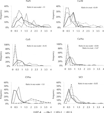
Fig. 11. Histogram of the frequency of occurrence of elemental ratios. Ratios from EDS are shown for cores 07-4 and 06-1. 03-1 and 02-5 were analyzed using IC-PMS. Sea-water and crust ratios from Reference Wilson, Riley and SkirrowWilson (1975) and Reference WedepohlWedepohl (1995).
The relationships seen in Figure 11 may indicate that the differences between EDS analysis and IC-PMS analysis render the comparison of these data impossible. However, it should be noted that EDS sampling of impurities was very random. A more detailed centimeter-by-centimeter comparison of IC-PMS and EDS chemistry from core 07-4 is being completed in order to better assess the differences between EDS and IC-PMS analysis. These data will also be used to examine the relationship between the physical and chemical characteristics within shallow firn in greater detail.
Conclusions
The characterization of physical properties in four cores from the US ITASE traverses of 2006 and 2007 (06-1, 06-2, 06-3 and 07-4) revealed site-specific details that would have been missed if only chemical characterization had been completed. Characterization of internal surface volume, S V, at site 07-4 and others showed that the progression from firn to ice is not entirely linear, as would be assumed if only grain size or porosity were considered. Further investigation of changes in S V with depth may aid in the understanding of the processes of firn densification and metamorphism in the ice sheet. The findings described above indicate the importance of characterizing multiple parameters to the understanding of ice cores as climate proxies.
The high degree of clustering of poles in sample 06-1-97 and the inclusion of a great number of low-angle misorientations indicate subgrain formation. Subgrains are not typically expected to form in the shallow parts of the ice sheet, but visual evidence of subgrain formation was found in samples as shallow as 50 m. These findings indicate that SEM and EBSD are valuable techniques for investigations of strain in the shallow parts of ice sheets.
The inter-regional trends in aerosol/particulate loading determined by EDS analysis of impurities are in accordance with those previously published from IC and IC-PMS data. The previously established patterns of Na and Ca deposition at Taylor Dome where Ca is primarily continental and Na is primarily marine (Reference De Angelis, Steffensen, Legrand, Clausen and HammerDe Angelis and others, 1997; Reference Legrand and MayewskiLegrand and Mayewski, 1997; Reference SteigSteig and others, 2000) and South Pole where both are primarily marine (Reference Tuncel, Aras and ZollerTuncel and others, 1989; Reference Legrand and MayewskiLegrand and Mayewski, 1997) were accurately determined using EDS. The differences in patterns of SO4 2− between the sites also indicate dissimilar SO4 2− sources (i.e. volcanic versus oceanic). In addition to accurately characterizing differences in loading and incorporation into the ice sheet, EDS analysis also identified the general trend of decreasing concentration with movement inland.
The morphology and microstructural location of impurities was found to be dependent upon the elements present. As was determined in previous studies (Reference Cullen and BakerCullen and Baker, 2001; Reference Obbard, Iliescu, Cullen and BakerObbard and others, 2003; Reference Barnes and WolffBarnes and Wolff, 2004; Reference Rosenthal, Saleta and DozierRosenthal and others, 2007; Reference Iliescu and BakerIliescu and Baker, 2008), the formation of filaments (FIL) was found to require the presence of marine species, whereas bright white spots (BWS) contained both marine and continental species. Not reported elsewhere is the characterization of filament tufts (TAN), which require the presence of continental (dust) species for their formation.
The analysis of both the soluble and insoluble chemistry and physical properties within a single firn or ice specimen suggests that both properties can provide valuable insights regarding environmental conditions at the time of deposition (temperature, atmospheric chemistry, atmospheric circulation patterns, etc.) and conditions affecting post-depositional incorporation into the ice sheet (micrometeorological differences, shallow firn metamorphism, accumulation hiatuses). Many of these properties are intricately linked and investigations of their relationships using SEM, EDS and EBSD will advance our understanding of the spatial and temporal changes in the climate of Antarctica in a way that no other instrumentation or technique could.
Acknowledgements
The US National Science Foundation (NSF) Office of Polar Programs is acknowledged for funding this project under OPP 0538494. Also acknowledged are participants of the 2006 and 2007 US ITASE traverses involved in the collection and preparation of ice cores for this research. C. Daghlian of the Dartmouth Medical School Electron Microscope Facility and S. Sneed of the University of Maine Climate Change Chemistry Laboratory are thanked for lending their time and expertise. A final thanks to reviewers T. Thorsteinsson and M. Tranter whose attention to detail and insightful comments greatly improved the quality of the manuscript.


