Performance of Location and Positioning Systems: a 3D-Ultrasonic System Case
Performance of Location and Positioning Systems: a 3D-Ultrasonic System Case
Volume 3, Issue 2, Page No 106-118, 2018
Author’s Name: Khaoula Mannay1,2,a), Jesus Urena1, Álvaro Hernández1, Mohsen Machhout3
View Affiliations
1Department of Electronics, University of Alcala, 28805, Alcalá de Henares, Madrid, Spain
2EµE Lab Faculty of Sciences of Monastir, National Engineer School of Tunis, University of Tunis EI Manar, 1002, Tunis, Tunisia
3EµE Lab, Faculty of Sciences of Monastir, University of Monastir, 5019, Monastir, Tunisia
a)Author to whom correspondence should be addressed. E-mail: khaoula.mannay@gmail.com
Adv. Sci. Technol. Eng. Syst. J. 3(2), 106-118 (2018); ![]() DOI: 10.25046/aj030213
DOI: 10.25046/aj030213
Keywords: Indoor Ultrasonic LPS, LPS distribution, 3D positioning, PDOP, Positioning error, Accuracy, LPS fusion

Export Citations
The necessity of navigation in people and mobile robots (MR) through specific environments (indoors or outdoors) has become more and more relevant nowadays. For indoors, generally speaking, the positioning systems can be divided into 2D (two dimensions) or 3D (three dimensions) approaches, where Ultrasonic Local Positioning Systems (ULPS) are often a common solution for MRs in 2D. This work proposes the extension of an already developed 2D ULPS to a 3D ULPS, where the compact design and the suitable performance of the initial 2D ULPS have been maintained. The ultrasonic beacons have been re-arranged to avoid co-planarity, then improving the third coordinate estimation. Furthermore, this work proposes the use of up to four ULPSs together to cover the 3D region of interest. Two configurations have actually been considered, one involving three ULPSs and another based on four. A heuristic Position Dilution of Precision (PDOP) estimation has been carried out, by taking into account two ways of obtaining the 3D-position: a) all beacons from the three different ULPSs are processed simultaneously, so all measurements are considered in the same set of positioning equations; and b) every ULPS is detected and considered separately and, later, the different estimated positions are merged. The second option is more likely to happen in a real scenario and, furthermore, the fusion of the independent positions obtained from each one of the ULPS improves the final position accuracy.
Received: 01 November 2017, Accepted: 21 February 2018, Published Online: 12 March 2018
1. Introduction
The necessity for positioning and navigating objects and people indoors and outdoors is expanding more and more every day. For outdoor environments, the Global Positioning System (GPS) is widely used. Nevertheless, whether there is a lack of RF signals, indoors or in constrained outdoor environments, other approaches have already emerged as a supporting and/or alternative technology, thus providing the so-called Local Positioning Systems (LPS). The demand for these LPSs, and in general terms for indoor positioning, has also become more relevant due to the worldwide spreading of smart devices, and their corresponding location applications.
Different sensory technologies have already been used in the development of LPS, such as Wi-Fi, infrareds (IR), ultrasounds (US) or radio-frequency (RF). The final decision on one technology or another is mainly related to the type of application, the environment, the required accuracy, as well as other secondary parameters [1] [2] [3]. Among them, ultrasounds-based approach is often considered whether the required accuracy is in the range of centimetres, not only for 2D but also for 3D deployments.
This work has been initially based on the previous LOCATE-US LPS (ULPS), firstly developed by the GEINTRA-US/RF Research Group from the University of Alcalá for 2D positioning [4]. A performance analysis of an ULPS is presented here when it is adapted for 3D positioning in a certain region. The proposal consists of using several ULPSs, which cover the area under scanning from different points of view in order to achieve an accurate estimation of the receiver’s position in 3D. The main goal of the paper is the study of different configurations of these ULPSs (number and location in the environment) and compare them in terms of the accuracy obtained in a grid of test points that cover all the 3D region of interest. As the positioning accuracy depends on the position itself to be determined, for every particular configuration it is necessary to study the positioning errors in all the points for all the cases. The rest of the manuscript is organized as follows: Section 2 presents a general background about LPSs, their main characteristics and technologies; Section 3 describes the previous LOCATE-US LPS, whereas the proposed 3-D ultrasonic LPS (ULPS) is presented in Section 4; Section 5 explains the 3D positioning algorithm implemented for the ULPS; Sections 6, 7 and 8 shows some simulation results; Section 9 presents a short discussion; and, finally, conclusions are considered in Section 10.
2. LPS Background
Local Positioning Systems (LPS) try to position one or multiple mobile objects accurately in an indoor environment. They are often used in applications, such as environment monitoring, people tracking, robot localization, resource management, or location-based services. The moving object is usually equipped with a small receiver (or transmitter depending on each LPS design), which acquires the emissions coming from the beacons forming the LPS, in order to estimate its own position. The nature of the transmitted signals can be different, depending on the technology involved: IR, RF, US, etc. [5]. According to this, Fig. 1 shows a general scheme for a LPS, where the beacons are fixed in the environment and the receiver is moving and computing its own position.
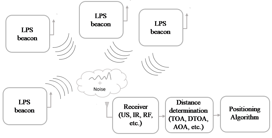 Fig. 1. General scheme of a LPS based on transmitting beacons and a moving receiver.
Furthermore, LPSs can also be classified into two groups: absolute for those where the mobile object is able to estimate its own position with respect to a reference point at any time; relative, when the mobile object can only know its position in a relative way to other receivers (or nodes) existing in the same coverage area [5].
Common LPS applications are those dedicated to 2D positioning and navigation of mobile robots and/or vehicles, as well as those focused on 3D positioning of smart devices and vehicles, such as smart phones, drones, etc. [7] [8]. Furthermore, Location-Based Services (LBS) are also potentially commercial applications for the market, not only to deliver context-dependent information accessible with a mobile device, but also to obtain information or navigate in the corresponding indoor environment. Finally, LPSs become particularly interesting in some emergency scenarios, such as positioning medical staff or equipment in hospitals, assisting rescue services in critical situations, or those proposals applied to intelligent transportation systems and/or industry manufacturing [9].
The final accuracy of a LPS in the position determination often depends on the system configuration, the sensory technology and the type and difficulty of the coverage area. Related to this, proposed LPSs are typically parametrized by the geometric dilution of precision (GDOP), where the distribution of the distance error between the estimated position and the true position is computed. Another key parameter is the range of coverage, where common values are between 5 meters and 50 meters. In this sense, for large coverage areas, scalability is key to guarantee an average positioning performance, as the positioning estimation degrades with the distance between the transmitters and receiver [10] [11] [12].
As far as the positioning algorithms are concerned, all of them are based on the determination of a variable from the beacon-receiver transmission. Some previous works based on ultra-wide band (UWB) have been recently proposed for indoor positioning by using the time differences of arrival (TDOA) from the RF transmissions between a reference beacon and the others. Typical accuracy values for these approaches are in the range of metres or even centimetres, although they present significant drawbacks, such as complexity or multi-path effects on the achieved accuracy [13] [14].
On the other hand, wireless local area networks (WLAN) have also been applied to indoor positioning [15]. Although they can also be based on TDOA, most cases deal with the received signal strength (RSS), reaching accuracies from 3m to 30m approximately [16] [17]. A similar case is the use of radio-frequency identification (RFID) [18]. In the case of infrareds, they often require a direct line-of-sight (LOS) communication between devices along a very short distance [19], where proximity, differential phase shift, and angle of arrival (AoA) are predominant.
Finally, ultrasounds-based systems also deal with TDOA [20], when there is no synchronization between the beacons and the receiver, and, afterwards, a hyperbolic positioning algorithm allows the position of the receiver to be estimated. The global accuracy of ultrasonic LPS (ULPS) is high and the structure is simple, but they often present drawbacks, such as multipath effects, Doppler, etc. [21] [22] [23].
3. General view of LOCATE_US system
The 2D LOCATE-US ULPS, designed by the GEINTRA-US/RF Research Group from the University of Alcala [4] [24], is a compact, light and portable ultrasonic beacon architecture [5]. The ULPS is formed of five coplanar ultrasonic beacons (Bi, where i=1,2,…5), placed at the four corners of a 0.707m x 0.707m square and at the centre, as is shown in Fig. 2. The five beacons have the same orientation (usually the ULPS is placed in the ceiling) and they cover roughly the same area on the floor. As the emission pattern of transducers is 120º [5], the ULPS can cover an area of 40m² roughly for a height of 3.5m. Any receiver inside the coverage area (attached to smartphones, a mobile robot (MR), a drone, …) can compute its position in an independent and autonomous way [4] [24].
In order to cover wide indoor areas, several ULPSs can be easily deployed. Particular calibration techniques have been proposed in [27] to facilitate this deployment.
The emitters in the ULPS use a code division multiple access (CDMA) and a time division multiple access (TDMA) protocols. Every emitter is encoded with a different code, with good auto-correlation properties and low mutual interference properties with the others. The ultrasonic transmissions of the different emitters can be configured in terms of sampling frequency, modulation schemes and code patterns to be emitted. The obtained accuracy for the measurement of distances is in the centimetre range (we assume a typical deviation of 1cm). The distances measured can be up to about 20m. All that is enough for MR applications in 2D spaces, and if extensive areas must be covered we can use a set of single ULPSs [4].
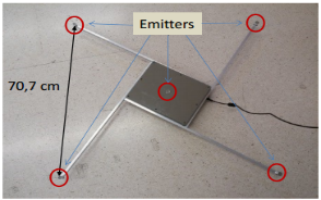 Fig. 2. General view of the 2D LOCATE-US LPS
4. Proposed 3D ULPS
The 3D ULPS described hereinafter is an extension of the 2D LOCATE-US, so it is also formed by five ultrasonic beacons Bi placed at the four vertices of a 0.707m x 0.70 m square and at the centre, as is shown in Fig. 3.a). All of them present slight variations in the z coordinate to improve this coordinate estimation and to avoid co-planarity; but still keeping the same properties of the previous 2D ULPS, such as the common orientation and coverage area. The new beacon distribution is: B2 and B4 are in the base plane, B3 and B5 are 10cm high from the base plane, and finally B1 is placed at 20cm high from the base plane [24].
The ultrasonic beacons are wired-synchronized to enable simultaneous and periodic emission [4] [24]. The ultrasonic transmission are encoded with orthogonal 1023-bit Kasami sequences, in order to mitigate any effect coming from multiple access interference (MAI) as much as possible [25]. These codes have been selected due to their suitable auto-correlation and cross-correlation properties. For their transmission, a binary phase shift-keying (BPSK) modulation has been carried out, with a carrier placed at the central frequency of the transducer bandwidth, fc=41.67kHz. Two carrier cycles per modulation symbol have been applied, and ultrasonic transmissions are carried out periodically every 50ms to reduce multipath effects.
The involved ultrasonic transducer is the Prowave 328ST160 [26], together with an ad-hoc front-end designed for this application. The five beacons Bi are managed by a FPGA-based system, in charge of controlling the global operation of the ULPS through an Ethernet link [24].The type of binary sequence and its length, the number of carrier periods, the type of carrier, and the time interval between different emissions can be configured by the PC. A digital pass-band filter with a 40 kHz central frequency and a 10 kHz bandwidth has been included to constrain information to the ultrasonic transducer bandwidth [26].
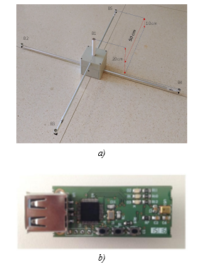 Fig. 3. a) General view of the 3D LOCATE-US LPS;
- b) Designed ultrasonic receiver.
With regard to the reception, the moving device estimates its position asynchronously by hyperbolic trilateration from the TDOA measurements between a reference beacon and the others. To detect the TDOAs, the mobile device demodulates the received signal and correlates it with the corresponding emitted Kasami sequences, based on a generalized cross-correlation (GCC) of the received signal. A main lobe appears at the arrival instant for every Kasami sequence, so it is possible to calculate the associated TDOAs. Finally, a Gauss-Newton minimization method computes the position. Fig. 3.b) shows the general aspect of the used ultrasonic receiver [24].
5. 3D Positioning
In positioning systems, it is important to know the accuracy of the estimated position, which depends on the quality of measurements (ranging distances, signal strength, etc.), and on the geometry of the positioning system (beacons’ geometry) with respect to the mobile node. The Position Dilution of Precision (PDOP) includes such dependencies and can be obtained empirically using (1).
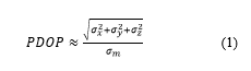 Where , and are the position variances in the three axes X, Y and Z, respectively; and is the standard deviation in the distance measurements (assumed to be 1cm hereinafter). As has been already mentioned, the technique used to position objects in 3D is based on the TDOAs, thus requiring synchronization between beacons (emitters), but not with receivers.
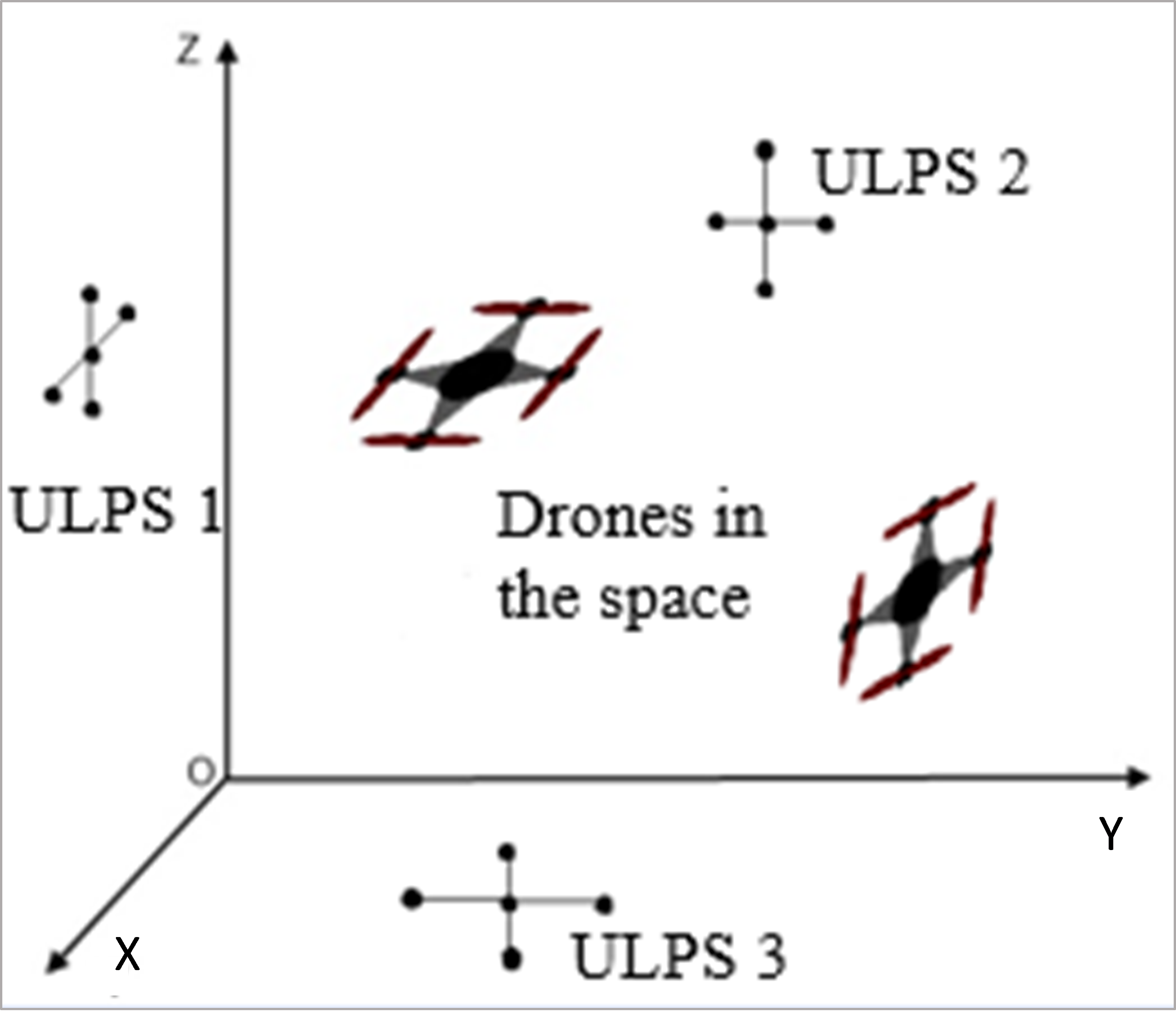 Fig. 4. Example of 3D configuration using three ULPSs and two receivers (drones).
In order to position a mobile target in a 3D space (see Fig. 4), a single ULPS is not enough to cover all the space with enough accuracy, assuming an 8x8x8m3 volume. The setup with a single ULPS implies that the performance significantly degrades with the height variation, due to the poor Vertical Dilution of Precision (VDOP), which determines the performance by only taking into account the typical deviation in the z coordinate.
Thereby, the use of only one ULPS is not a suitable solution. As an example of that, Fig. 6 shows the case in which one ULPS is placed at the centre of the floor at coordinates (4m, 4m, 0m), whereas Fig. 8 depicts the case of one ULPS placed at the lower corner with coordinates (0m, 0m, 0m). Both Figs. represent the cloud of obtained position points, assuming the receiver in the X-Y plane (with steps of 1m in both axes), for three different heights: z=6m in the half upper volume of the room; z=4m in the middle of the room; and z=2m in the half lower volume of the room.
Additionally, Figs. 7 and 9 show the different PDOP values for the same X-Y planes and heights (z=2m, 4m, 6m). Note that the PDOP values are high in general terms (above 100). The contour map is a representation of the PDOP in planes at different height. The values of the PDOPs have been calculated for every point in the grid (according to the cloud of points with the estimated positions after the simulations).
Each color represent a particular value of PDOP; and the greater the PDOP the greater the positioning error in this point (even in the case that all the distances has been measured always with a typical deviation of 1 cm). With this representation one can have an idea about the error we can wait in each region of the environment in a real situation with a particular ULPS arrangement.
On the other hand, the receiver has been placed at every point in a 9x9x9 grid (8x8x8m3 volume using 1m interval). At each point, a hundred simulations have been run by using an hyperbolic trilateration with the Gauss-Newton Positioning Method (GNPM) [10]; the standard deviation in the distance measurements is =1cm, which is consistent with ultrasonic measurements of distances.
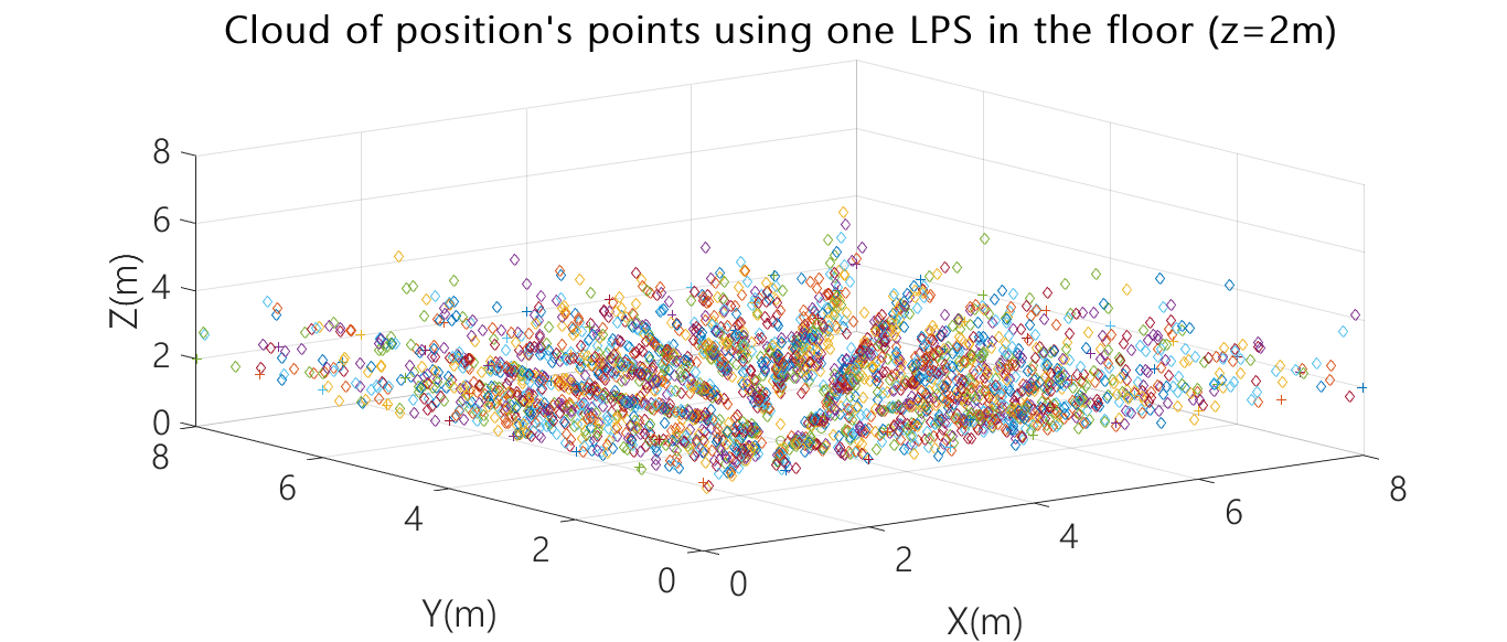
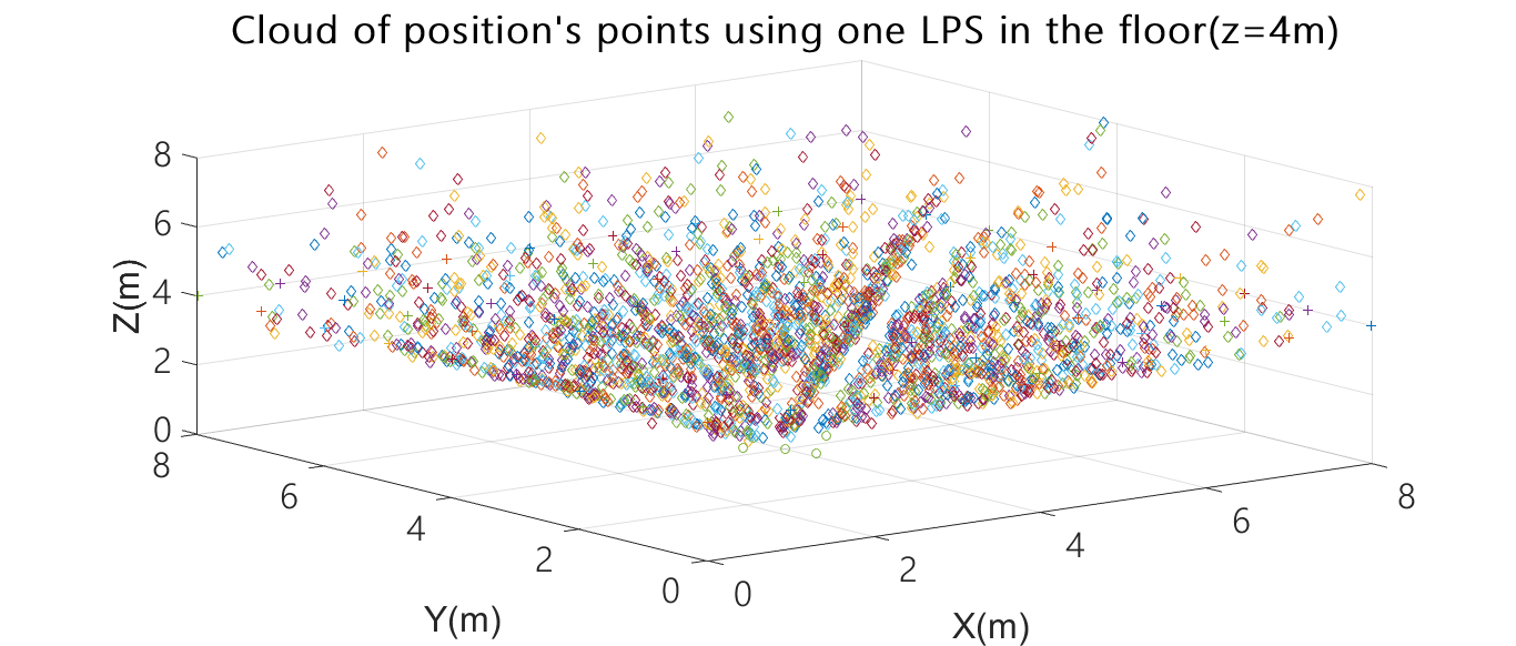
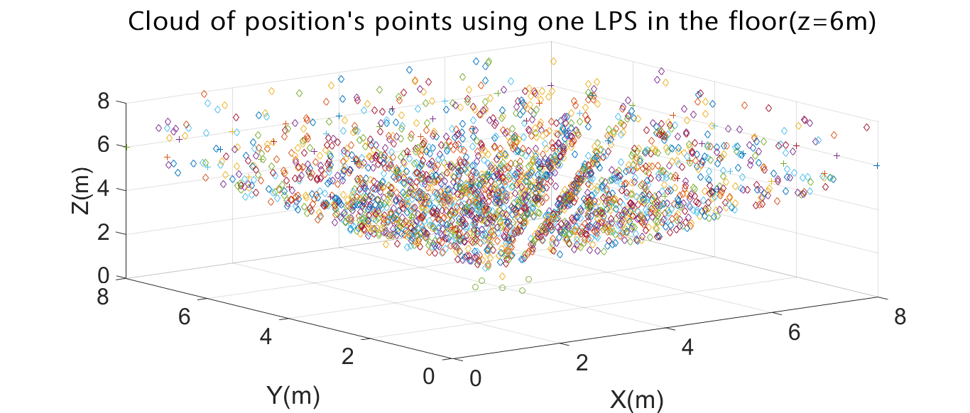 Fig. 6. Cloud of position points for one ULPS placed at the centre of the floor (4m,4m,0m) for X-Y planes at different heights (z=2m, z=4m, z=6m).
As can be observed in Fig. 7, the PDOP values differ from one plane to another, but, in general, it is smaller in the centre of every plan, and then it increases towards the sides of the room. For the first plane z=2m (lower half of the room), the PDOP varies from 100 to 900.
Whereas these values increase in the middle of the room (z=4m), where the PDOP is between 250 and 800; and, finally, they range from 450 to 850 in the third plane z=6m (upper half of the room).
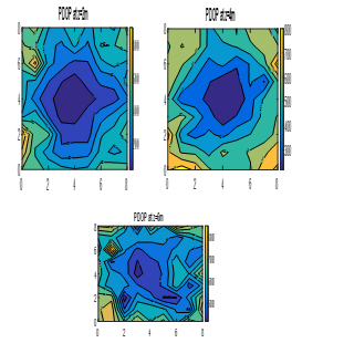 Fig. 7. Colour map of PDOPs for an ULPS placed at the centre of the floor (4m, 4m, 0m) for different X-Y planes (z=2m, z=4m, z=6m).
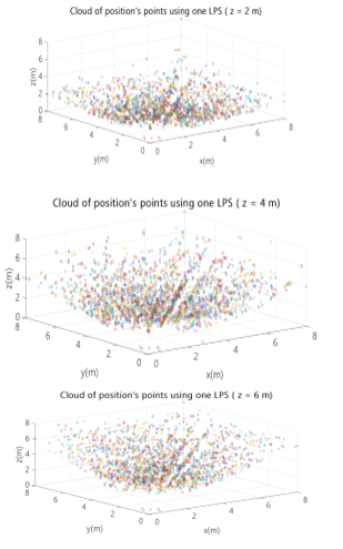 Fig. 8. Cloud of position points using an ULPS placed at (0m, 0m, 0m) corner for X-Y planes z=2m, z=4m and z=6m.
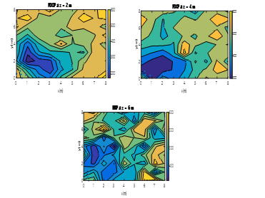 Fig. 9. Colour map of PDOPs for an ULPS placed at (0m, 0m, 0m) corner for X-Y planes (z=2m, z=4m, z=6m).
Similar conclusions can be derived from Fig. 9 with the LPS placed at corner (0m, 0m, 0m) and pointing at the centre of the room. For the first plane z=2m, the PDOP values are between 200 and 600; for z=4m, they are between 300 and 600; and between 420 and 600 for z=6m.
In order to improve these results, as well as to enhance the coverage area, the use of several ULPSs placed at different points of the room has been considered. These tests have been carried out by using two different configurations:
- Configuration A: three ULPSs placed at the centres of X-Y plane z=0m, Y-Z plane x=0m and X-Z plane y=8m, respectively. All these ULPS are emitting perpendicularly to the plane in which they are placed.
- Configuration B: four ULPSs placed at corners (0m, 0m, 0m), (8m, 8m, 8m), (0m, 8m, 0m) and (8m, 0m, 8m), respectively. Each LPS is emitting in the direction of the cube diagonal corresponding to the corner at which it is placed.
In practical situations, the 3D position can be computed with one or an array of microphones to cover all the incoming signals. In this way, two options have been considered here:
- Simultaneous measurements: all the distances (derived from TDOAs), from all the ULPSs that must be synchronized, are obtained at the same time, so the positioning algorithm involves as many equations as measured distances. For the three ULPSs configuration, the positioning algorithm requires fifteen equations, whereas, in the four ULPSs configuration, twenty equations.
- Independent measurements for each ULPS: whether five distances from one single ULPS are obtained at the receiver, it obtains a 3D position. In parallel, several 3D positions can be computed (one per every detected ULPS). To combine all these 3D positions, the Maximum Likelihood Estimation (MLE) is applied. In the case of having available three independent measurements q1, q2 and q3 for a certain position q, provided that the positioning error may be modelled as p(qi|q)=N(q, σi), the merged estimate for position q can be obtained by following the procedure (2):
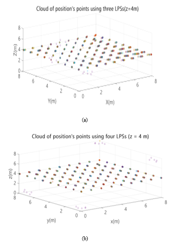 Fig. 10. Cloud of position points for the X-Y plane z=4m using: (a) configuration A with three ULPSs; (b) configuration B with four ULPSs.
Where q1, q2 and q3 are three independent measurements for position q in the case of detecting three different ULPSs. Since the statistical information is additive, the new standard deviation σ will be (3):
Where s1, s2 and s3 are the standard deviations for the corresponding position measurements q1, q2 and q3.
6. Results for configuration A (three ULPSs on the walls)
In order to compare the performance of each ULPS arrangement and the total number of distance measurements available, for both configurations A and B, one hundred simulations have been conducted at every point in the 3D grid (9x9x9m3) with a step in x, y and z of 1m. The standard deviation considered in the distance measurements is =1cm.
6.1. Simultaneous measurements from all ULPSs
In this case, the 3D receiver position is estimated by the GNPM at each point, assuming there are available simultaneous measurements of TDOAs from all the ULPSs at the receiver. For configuration A, the space is covered by three ULPSs, as shown in Fig. 10. Two cases have been studied: only two of them are available; all the three are available.
- Two ULPSs available
Firstly, in addition to the ULPS placed at the position (4m, 4m, 0m), a second ULPS has been placed at the centre of the wall y=8m, at position (4m, 8m, 4m). Figs. 11 and 12 show the cloud of positions obtained, as well as the PDOP for planes z=2m, z=4m and z=6m.
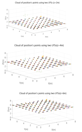 Fig. 11. Cloud of position points for two ULPSs: one placed at (4m, 4m, 0m) and the other at (4m, 8m, 4m), for different X-Y planes (z=2m, z=4m, z=6m).
Comparing with the previous results achieved with only one ULPS (Figs. 6 to 9), the improvement is clear: now the PDOP varies from 5 to 100, providing larger volumes with lower values. The lowest PDOP values are around the centre of the room.
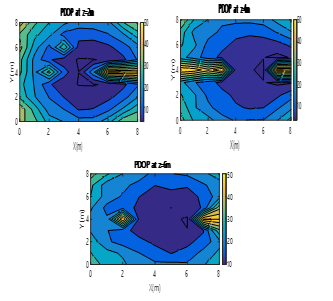 Fig. 12. Colour map of PDOP values for two ULPSs placed at (4m, 4m, 0m) and the other at (4m, 8m, 4m), for different X-Y planes (z=2m, z=4m, z=6m).
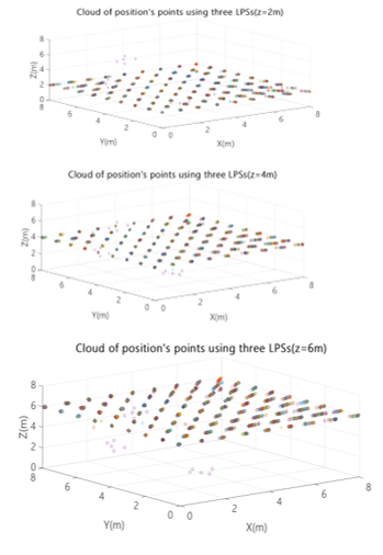 Fig. 13. Cloud of position points for three ULPSs placed at (4m, 4m, 0m), (4m, 8m, 4m) and (0m, 4m, 4m) for different X-Y planes (z=2m, z=4m and z=6m).
- Three ULPSs available
A third ULPS has been added at coordinates (0m, 4m, 4m). Figs. 13 and 14 show the same clouds of points and PDOPs as before, for X-Y planes z=2m, z=4m and z=6m.
By adding the third ULPSs, the cloud of the 100 position points simulated is more accurate around the real positions considered in the grid. The PDOP values decrease below 30 in general terms, and below 15 in almost all the space, independently of the height.
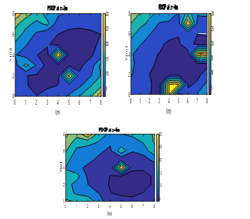 Fig. 14. Colour map of PDOP values for three ULPSs placed at (4m, 4m, 0m), (4m, 8m, 4m) and (0m, 4m, 4m) for different X-Y planes (z=2m, z=4m, z=6m).
6.2. Independent measurements for each ULPs
- Fusion of two ULPSs
The configuration analysed here is the same as that one in Section 5.1.1. Now, the 3D positions from the two different ULPSs are obtained separately, and, afterwards, these positions are combined by using a MLE to estimate a final position. The process has been repeated a hundred times at each point in the aforementioned grid. The final PDOP values are shown in Fig. 15, varying from 5 and 100, also providing large areas with low values. It is worth noting that these results are similar to those in Fig. 12 for the case of simultaneous measurements.
- Fusion of three ULPSs
When having a third ULPS placed at (4m, 0m, 4m), the PDOP values have been calculated for a hundred simulations at each point in grid, and they are shown in Fig. 16. Again, the distribution of the PDOP values with the MLE merging method are very close to the case when using simultaneous measurements (see Fig. 14).
In order to summarize the results for the case analysed in this section, for the whole volume under analysis the Cumulative Distribution Function (CDF) of the position error has been obtained, by taking into account all the points in the grid (100 simulations per each position). Fig. 17 shows the CDF for simultaneous (a) and independent (b) measurement approaches.
According to Fig. 17, for simultaneous measurements, in the 90% of the cases the error is below 0.7m when using only one ULPS, below 0.2m with two ULPSs, and below 0.1m for three ULPSs. On the other hand, for independent measurements, in the 90% of the cases the error is below 0.9m for one ULPS, 0.8m for the fusion of two LPSs, and 0.7m for the fusion of three ULPSs.
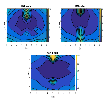 Fig. 15. Colour map of the PDOP values obtained by the MLE when using two ULPSs at (4m, 4m, 0m) and at (4m, 8m, 4m) for X-Y different planes (z=2m, z=4m, z=6m).
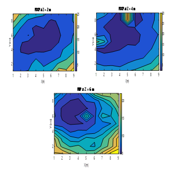 Fig. 16. Colour map of the PDOP values obtained by the MLE when using three ULPSs at (4m, 4m, 0m), (4m, 8m, 4m) and (0m, 4m, 4m) for X-Y different planes (z=2m, z=4m, z=6m).
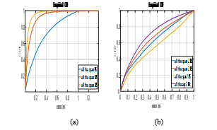 Fig. 17. CDF for the position error in the whole volume: a) using simultaneous measurements; and b) using independent measurements (and fusion).
7. Results for configuration B (with four ULPSs)
As has been already explained in Section 4, the whole volume is covered by four ULPSs in the configuration B. The goal is to improve the results presented in Figs. 8 and 9, where only one ULPS located at position (0m, 0m, 0m) was used.
7.1. Simultaneous measurements
- Two ULPSs
Together with the ULPS located at (0m, 0m, 0m), a second one is added at the opposite corner, that is, located at (8m, 8m, 8m). The resulting clouds of points and PDOP after 100 simulations at each grid point are shown in Figs. 18 and 19, respectively, for planes z=2m, z=4m and z=6m.
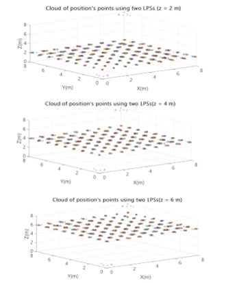 Fig. 18. Cloud of position points for two ULPSs at corners (0m, 0m, 0m) and (8m, 8m, 8m) for planes (z=2m, z=4m, z=6m).
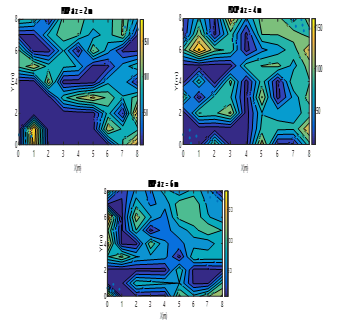 Fig. 19. Colour map of PDOP values for two ULPSs at (0m, 0m, 0m) and at (8m, 8m, 8m) for X-Y planes (z=2m, z=4m, z=6m).
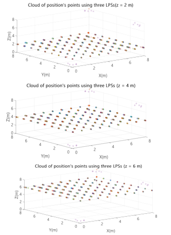 Fig. 20. Cloud of position points for three ULPSs, placed at (0m, 0m, 0m), (8m, 8m, 8m) and (8m, 0m, 8m) for X-Y planes z=2m, z=4m and z=6m.
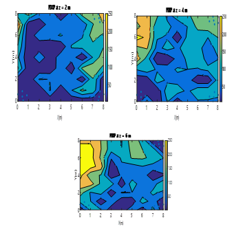 Fig. 21. Colour map of PDOPs for three ULPSs at (0m, 0m, 0m), (8m, 8m, 8m) and (8m, 0m, 8m) for X-Y planes (z=2m, z=4m,z=6m).
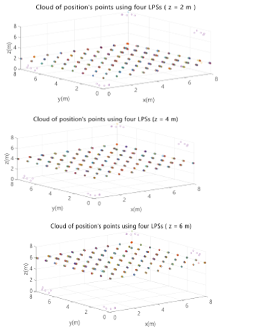 Fig. 22. Cloud of position points for four ULPSs at (0m, 0m, 0m), (0m, 8m, 0m), (8m, 0m, 8m) and (8m, 8m, 8m) for X-Y planes (z=2m, z=4m, z=6m).
It can be observed that there is an improvement in the error for all the grid points, compared to the case of only one ULPS, but still the PDOP values are in the interval from 10 to 180.
- Three ULPSs
With a third ULPS placed at the corner (0m, 8m, 0m), the obtained results are shown in Figs. 20 and 21, also for the three planes z=2m, z=4m and z=6m.
The 3D positions are now more accurate, since the errors decrease especially in the neighbourhood of the ULPSs. The PDOP values are below 50 in large areas of the analysed planes.
- Four ULPSs
Finally, a fourth ULPS is inserted at (0m, 8m, 0m), in addition to the previous three ones. The corresponding results are plotted in Figs. 20 and 21.
The errors have been considerably reduced with PDOPs between 5 and100, including large areas below 20.
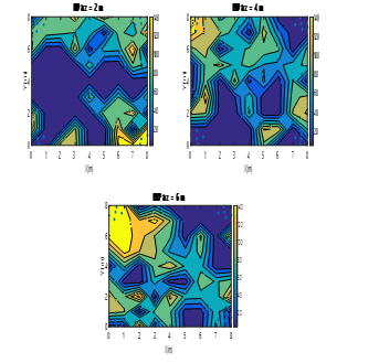 Fig. 23. Colour map of PDOP values for four ULPSs at (0m, 0m, 0m), (0m, 8m, 0m), (8m, 0m, 8m) and (8m, 8m, 8m) for X-Y planes (z=2m, z=4m, z=6m).
7.2. Independent measurements
In the second case analysed with the configuration B, each ULPS is considered independently. Figs. 24, 25 and 26 represent the PDOP values for two, three or four ULPSs,
respectively, after the fusion of the independent calculations for the positions.
Note that for two ULPSs the PDOP values are still as high as 420 in relatively large areas around the centre of the space. These areas are greatly reduced with three ULPSs (see Fig. 25) and even more with four ULPSs (see Fig. 26).
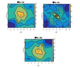 Figure 24. Colour map of the PDOP values obtained by the MLE when using two ULPSs placed at (0m,0m,0m) and (8m,8m,8m) for different X-Y planes (z=2m, z=4m, z=6m).
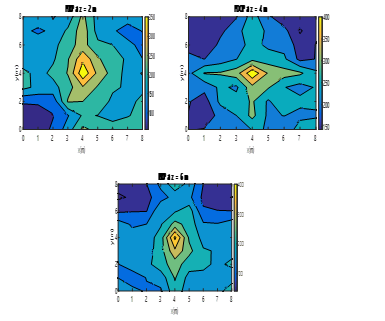 Figure 25. Colour map of the PDOP values obtained by the MLE when using three ULPSs placed at (0m,0m,0m), (8m,8m,8m) and (0m,8m,0m) for different planes (z=2m, z=4m and z=6m).
- Error CDF
The error CDF, again obtained in all the points (and for a hundred simulations at each) for these distributions of ULPSs previously described, can be seen in Fig. 27. The upper plot considers simultaneous measurements, whereas the second one involves the fusion of independent measurements from each ULPS. In both, different CDF plots are shown for one, two, three and four ULPSs.
For the simultaneous emission, the errors for the 90% of the cases are below 0.75m using one ULPS, 0.15m for two ULPSs, 0.1m for three ULPSs and, finally, 0.07m for four LPSs (see Fig.27.a). In case of fusion of data from independent ULPSs, these errors are below 0.85m for one ULPS and below 0.7m for four ULPSs (see Fig. 27.b).
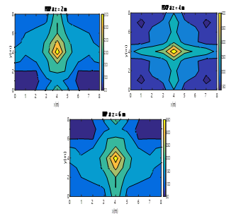 Figure 26. Colour map of the PDOP values obtained by the MLE when using four ULPSs placed at (0m,0m,0m), (8m,8m,8m), (8m,0m,8m) and (0m,8m,0m) for different X-Y planes (z=2m, z=4m, z=6m).
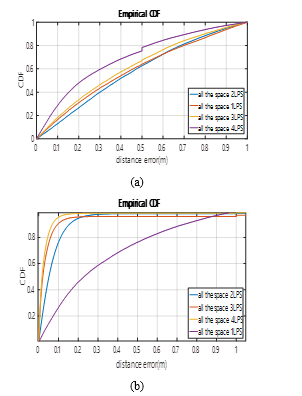 Figure 27. Error CDF in all the space, for 1, 2, 3 or 4 ULPSs and considering: a) simultaneous measurements with all the ULPSs; and b) independent measurements from each ULPS.
Finally, for the best case (simultaneous measurements with four ULPSs), the CDF has been split and represented in Fig. 28 for the points in every analysed plane z=0m, 1m, 2m …8m. Note that
the error is quite similar in all the planes and, for the 90% of the cases, it is below 6-8 cm. That is, the performance of the system is similar in the whole volume.
8. Experiment results
In order to validate the proposal with real data, firstly, configuration A presented in Section 5 has been considered by using one ULPS. The tests have been carried out by positioning a receiver at each one of the 16 specific positions in a grid on the floor, as can be observed in Fig. 29. The ULPS is placed in the ceiling at a height of 3.5m. This workspace is not very complex and only the points of the corners of the grid have some problems due to signal attenuation and multipath.
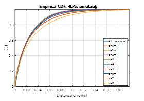 Fig. 28. Error CDF in every X-Y plane (z=1,2,…,8) for 4 ULPSs with simultaneous measurements.
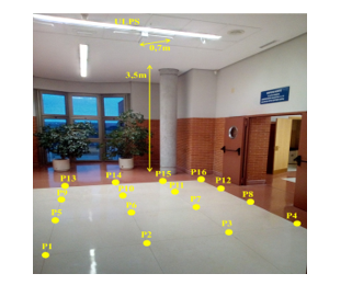 Fig. 29. Experimental setup formed by one ULPS placed in the ceiling at a height of 3.5m and the receiver placed at 16 points in a 4x4m² grid on the floor.
A set of 100 measurements have been carried out for every position, where the final estimated positions are represented by blue crosses in Fig. 30. On the other hand, the red circles are the real positions. An error ellipse containing the 95% of estimates has also been represented for every cloud of points. The green diamonds are the beacons’ projections on the floor. It can be observed that the estimated positions at the test points below the beacons have a lower error than those further away. Nevertheless, all the positions are reasonably estimated.
Fig. 31 shows the error CDF obtained by simulating only one ULPS for the grid of points at z=3.5m. It can be observed that, for the 90% of cases, the positioning error is less than 1 cm. On the other hand, Fig. 32 represents a similar CDF for experimental data, considering all the measurements or grouping them into two subsets: points P6, P7, P10 and P11 (placed at the center of the grid, just below the ULPS) and the rest of points. The differences between simulated and experimental data can be due to several factors: inaccuracies in the position of the receiver when tests were performed, and propagation effects not considered in simulations (attenuation, multipath, non-Gaussian noise, etc.).
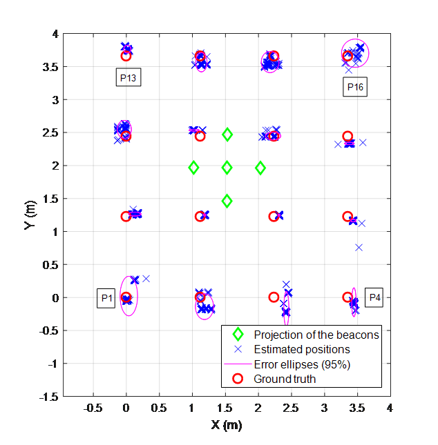 Fig. 30. Experimental test positions (red circles), estimated positions (blue crosses), and beacons’ projections (green diamonds)
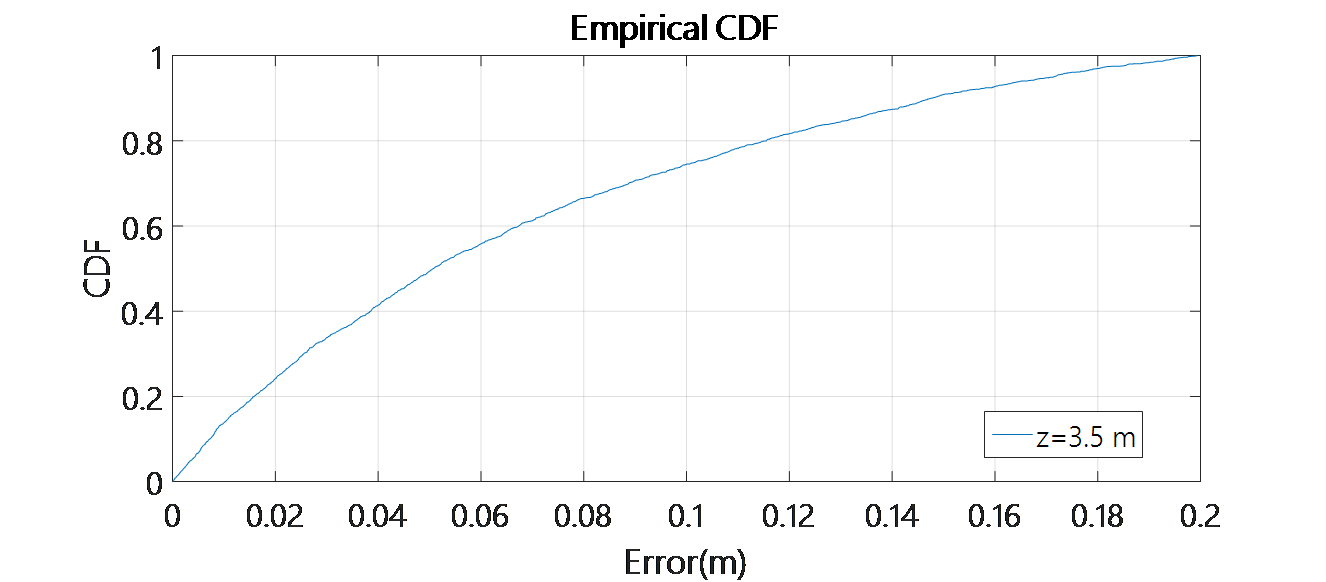 Fig. 31. Error CDF obtained by simulation for the X-Y plane (z=3.5m) using only one ULPS.
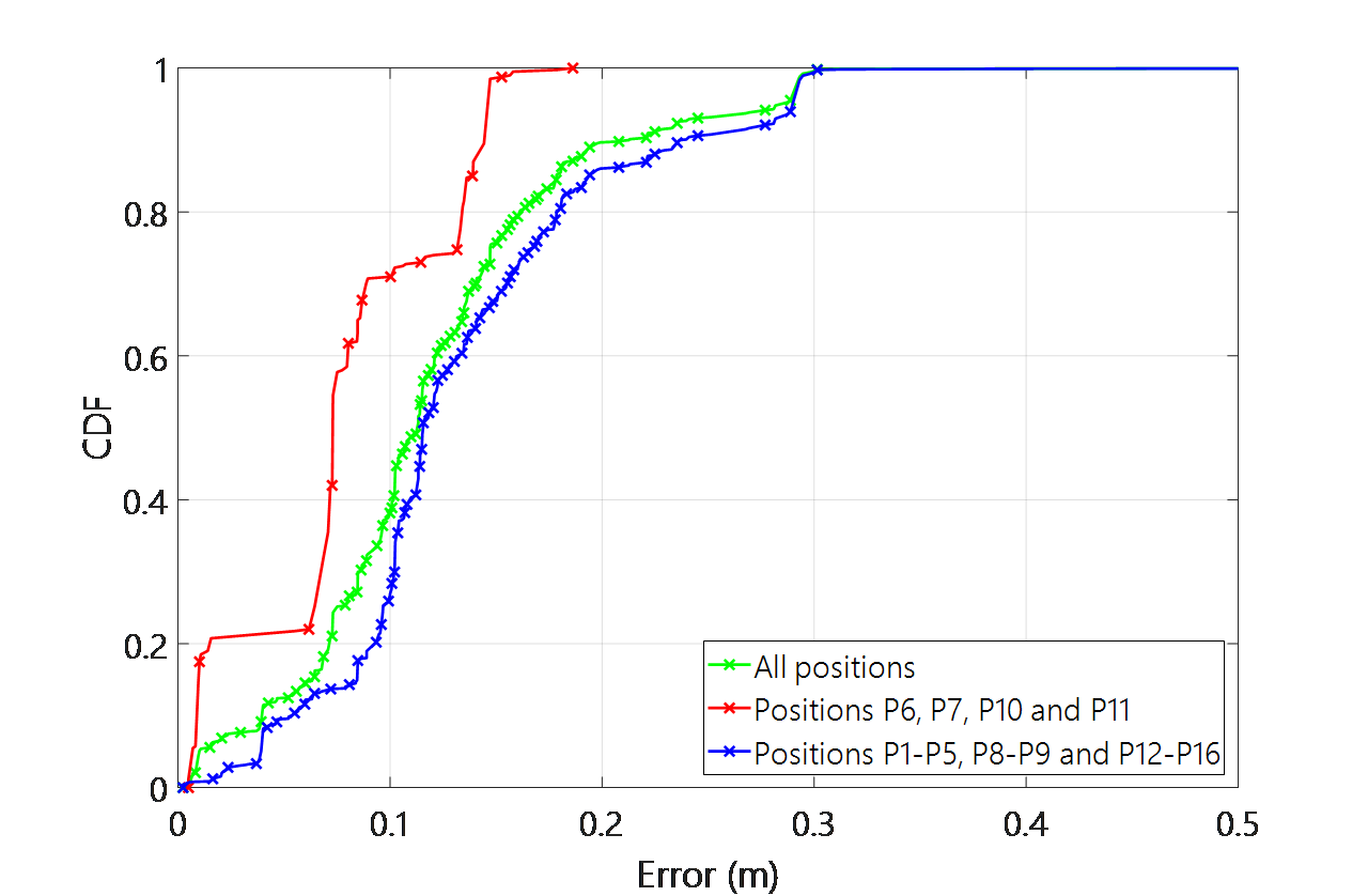 Fig. 32. Error CDF for the experimentally estimated positions in the X-Y plan (z=3.5m) using one ULPS.
Note that, according to the different CDFs in Fig. 32, the error is less than 20cm in the 90% of cases when considering all the test positions. This error is smaller (about 15cm) for those points just below the ULPS, whereas larger (in the range of 25cm) for the test
positions that are far away from the ULPS’ projection.
9. Discussion
When an ULPS is used in 2D, its final position can be fixed at the ceiling with all the beacons emitting downwards and the targets with receivers pointing upwards. In that case, the coverage area on the floor is a circle about 40m², assuming the ULPS is placed 3.5m high. For an extended 2D workspace, it is needed to add more ULPSs at the ceiling at different positions to cover a larger area on the floor. Anyway, these different ULPSs are always placed in the ceiling, they work independently and the obtained accuracy is similar for all the 2D floor positions considered.
Nevertheless, for a 3D positioning it is necessary to cover all the space and not only the floor surface. This is why a set of ULPSs must be placed at different positions and with different orientations (see Fig. 4) to cover all the space, thus having enough accuracy in all the volume of interest.
Two different configurations for 3D positioning in a cubical region of 8x8x8m3 have been studied in this work. The first is the configuration A with three ULPSs pointing towards the centre of the cube and placed at the centres of the X-Y plane (z=0m), the Y-Z plane (x=0m), and the X-Z plane (y=8m). The second is the configuration B with four ULPSs pointing towards the centre of the cube and placed at corners (0m, 0m, 0m), (8m, 8m, 8m), (0m, 8m, 0m) and (8m, 0m, 8m).
Furthermore, two alternatives have been considered for each configuration:
- To have measurements from all the ULPSs simultaneously (with all the emitters synchronized). In this case, all the measured distances can be provided to the positioning algorithms.
- To have measurements independently for each ULPS (avoiding the need of synchronization among the different ULPSs). In this case, a position is estimated for every ULPS and afterwards all the results are merged.
The use of simultaneous measurements from different ULPSs is better in terms of the obtained accuracy, but it requires synchronization among ULPSs, as well as a wide receiver coverage that can be difficult in practical systems. On the other hand, with independent measurements for each ULPS, these issues can be avoided at the cost of reducing accuracy (that can still be enough for many applications).
10. Conclusions
The performance of a 3D ultrasonic positioning system (ULPS), firstly developed with a structure and characteristics for 2D positioning, has been studied and adapted to be deployed for 3D positioning. The study has covered the use of different ULPSs configurations, considering simultaneous or independent measurements. The comparison has been carried out and based on the estimation of the PDOP, by using a grid that covers all the space of interest (a cube of 8x8x8 m3).
The achieved accuracy varies in the two cases analysed (case A and case B), depending on the number of ULPSs involved (1 to 4 ULPSs) and their positions/orientations (at the corners, in the ceiling, in walls….). Some preliminary experimental tests have also shown the performance for a single ULPS. The positioning error is less than 20cm for the 90% of considered measurements. This centimetre accuracy is in accordance with other positioning systems based on ultrasounds as can be observed in [5], which also compares this technology with others also applied to this type of systems.
Acknowledgment
This work has been possible thanks to the Spanish Ministerio de Economía, Industria y Competitividad (TARSIUS, ref. TIN2015-71564-c4-1-R, and SOC-PLC, ref. TEC2015-64835-C3-2-R) and the University of Alcala (LOCATE-US, ref. CCG2016/EXP-078). Authors thank Dr. David Gualda for his support with experimental measurements.
- Li, L. Feng, A. Yang, “Fusion Based on Visible Light Positioning and Inertial Navigation Using Extended Kalman Filters”, Sensors (Basel). 2017 May; 17(5): 1093. doi: 10.3390/s17051093
- M. Metev and V. P. Veiko, Laser Assisted Microtechnology, 2nd ed., R. M. Osgood, Jr., Ed. Berlin, Germany: Springer-Verlag, 1998.
- Curran, E. Furey, T. Lunney, J. Santos, “An Evaluation of Indoor Location Determination Technologies”, Journal of Location Based Services, vol. 5, no. 2, pp. 61-78, 2011.
- Gualda, J. Ureña, J. C. García and A. Lindo, “Locally-Referenced Ultrasonic-LPS for Localization and Navigation”, Sensors, vol. 14(11), pp. 21750-21769, 2014.
- Mautz, Indoor Positioning Technologies, Habilitation Thesis, ETH Zurich, 2012.
- Alarifi, A Al-Salman, M. Alsaleh, A. Alnafessah, S. Al-Hadhrami, M. A. Al-Ammar, H. S. Al-Khalifa, “Ultra-Wideband Indoor Positioning Technologies: Analysis and Recent advances”, Journal of Sensors 2016
- Parnian, Integration of Local Positioning System & Strapdown Inertial Navigation System for Hand-Held Tool Tracking, Habilitation Thesis, University of Waterloo, 2008.
- Sameshima, E. P. Katz, “Experiences with Cricket/Ultrasound Technology for 3-Dimensional Locationing within an Indoor Smart Environment Harry”, Technical Report, Carnegie Mellon University, 2009.
- Pahlavan, X. Li, and J. P. Makela, “Indoor geolocation science and technology”, IEEE Communications Magazine, vol. 40, no. 2, pp. 112-118, 2002.
- Roos, P. Myllymaki, H. Tirri, P. Misikangas, J. Sievanen, “A probabilistic ap-proach to WLAN user location estimation” International Journal of Wireless Information Networks, July 2002, Volume 9, Issue 3, pp 155–164
- Bodhi, M, Goraczko, The Cricket Indoor Location System, PhD Thesis, Massachusetts Institute of Technology, 2005.
- Mannay, J. Ureña, Á. Hernández, D. Gualda, J. M. Villadangos,” Analysis of performance of Ultrasonic Local Positioning Systems for 3D Spaces”, 2017 International Conference on Indoor Positioning and Indoor Navigation (IPIN). pp. 1-4. (ISBN 978-4-86049-074-4).
- Zhou, C. L. Law, Y. L. Guan and F. Chin, “Indoor Elliptical Localization Based on Asynchronous UWB Range Measurement”, IEEE Trans. on Instrumentation and Measurement, vol. 60, no. 1, pp. 248-257, 2011.
- García, P. Poudereux, A. Hernández, J. J. García and J. Ureña. “DS-UWB indoor positioning system implementation based on FPGAs”, Sensors and Actuators A: Physical, vol. 201, pp. 172-181, 2013.
- Prieto, S. Mazuelas, A. Bahillo, P. Fernandez, R. M. Lorenzo and E. J. Abril, “Adaptive data fusion for wireless localization in harsh environments”, IEEE Trans. on Signal Processing, vol. 60(4), pp. 1585-1596, 2012.
- Ocaña, M. A. Sotelo, L. M. Bergasa, R. Flores, “Low level navigation system for a POMDP based on WiFi and ultrasound observations”, Proc. of the 2005 IEEE International Symposium on Computational Intelligence in Robotics and Automation, (CIRA’05), pp. 335–340, 2005.
- Álvarez, M. E. De Cos Gómez, J. Lorenzo, F. Las-Heras, “Evaluation of an RSS-based indoor location system”, Sensors and Actuators, A: Physical, vol. 167 (1), pp. 110–116, 2011.
- D. Koutsou, F. Seco, A. R. Jimenez, J. O. Roa, J. L. Ealo, C. Prieto, J. Guevara, “Preliminary localization results with an RFID based indoor guiding system”, Proc. of the 2007 IEEE International Symposium on Intelligent Signal Processing (WISP’07), pp. 1–6, 2007.
- M. Gorostiza, J. L. Lázaro Galilea, F. J. Meca Meca, D. Salido Monzú, F. Espinosa Zapata and L. Pallarés Puerto, “Infrared sensor system for mobile-robot positioning in intelligent spaces”, Sensors, vol. 11(5), pp. 5416-5438, 2011.
- Ruíz, J. Ureña, J. C. García, C. Pérez, J. M. Villadangos, E. García, “Efficient trilateration algorithm using time differences of arrival”, Sensors and Actuators A: Physical, vol. 193, pp. 220-232, 2013.
- M. Villadangos, J. Ureña, J. J. García, M. Mazo, A. Hernández, A. Jiménez, D. Ruíz, C. De Marziani, “Measuring Time-of-Flight in an Ultrasonic LPS System Using General Generalized Cross-Correlation”, Sensors 2011, vol. 11, pp. 10326-10342, 2011.
- Gualda, Mª C. Pérez, J. Ureña, J. C. García, D. Ruiz, E. García and A. Lindo, “Ultrasonic LPS Adaptation for Smartphones”, International Conference on Indoor Positioning and Indoor Navigation (IPIN’13), pp. 1-6, 2013.
- Lindo, MC. Perez, J. Urena, D. Gualda, E. Garcia and J. Manuel Villadangos, “Ultrasonic signal acquisition module for smartphone indoor positioning”, Proc. of 2014 IEEE Conference on Emerging Technology and Factory Automation (ETFA), pp. 1-4, 2014.
- Hernández, E. García, D. Gualda, J. M. Villadangos, F. Nombela, J. Ureña, “FPGA-based Architecture for Managing Ultrasonic Beacons in a Local Positioning System”, IEEE Trans. on Instrumentation and Measurement, vol. 66, no. 8, pp. 1954-1964, 2017.
- Kasami, “Weight distribution formula for some class of cyclic codes,” Technical reportR-285, Coordinated Science Lab. University of Illinois, April 1968.
- Pro-Wave Electronics Corporation, Air Ultrasonic Ceramic Transducers 328ST/R160, Product Specification, 2014.
- Gualda, J. Ureña, J.C. García, J. Alcalá, A.N. Miyadaira. “Calibration of Beacons for Indoor Environments based on a Map-Matching Technique”. 2016 International Conference on Indoor Positioning Systems. pp. 1-7, Alcalá de Henares, Spain, October 2016.