Yuki Kato![]() | Guanming Guo
| Guanming Guo![]() | Masaya Kamigaki
| Masaya Kamigaki![]() | Kenmei Fujimoto
| Kenmei Fujimoto![]() | Mikimasa Kawaguchi
| Mikimasa Kawaguchi![]() | Keiya Nishida
| Keiya Nishida![]() | Masanobu Koutoku
| Masanobu Koutoku![]() | Hitoshi Hongou
| Hitoshi Hongou![]() | Haruna Yanagida
| Haruna Yanagida![]() | Yoichi Ogata*
| Yoichi Ogata*![]()
© 2023 IIETA. This article is published by IIETA and is licensed under the CC BY 4.0 license (http://creativecommons.org/licenses/by/4.0/).
OPEN ACCESS
The detailed understanding of heat transfer in the pulsating airflow in the pipe is critical to reducing heat losses in the engine exhaust stream and improving catalyst performance. In the present investigation, we have scrutinized the impact of pulsation frequencies ranging from 0-90 Hz on the flow velocity field and the consequent heat transfer through a horizontal pipe wall. The Nusselt numbers were evaluated at three distinct cross-sectional points moving from upstream to downstream, by systematically modulating the frequency. Temporal variations in the velocity field and temperature were captured utilizing particle image velocimetry (PIV) and dual-thermocouple probes, respectively. Intriguingly, while the Nusselt number for steady flow at 0 Hz closely adhered to Gnielinski’s equation, the pulsating flow demonstrated a peak between 25-35 Hz, a pattern not predicted by the prevailing quasi-steady-state theory. The observed frequency response of turbulence was found to be congruous with the Nusselt number, indicating that the heightened heat transfer at frequencies of 25-35 Hz could be attributed to the enhanced turbulence and the temperature gradient between the fluid and the wall surface during the deceleration phase in the hysteresis of turbulence in the pulsating flow. The unique frequency characteristics of heat transfer that were uncovered in this study, with respect to both flow velocity and temperature, offer valuable insights for devising strategies to mitigate heat loss during ignition and idling. Furthermore, these findings provide robust benchmarks for validating numerical simulations of pulsating flows in real-life automotive engines.
pipe flow, pulsation, turbulent flow, particle image velocimetry, heat transfer, Nusselt number, forced convection
The importance of heat transfer in pulsating flows is underscored by its ubiquity in various engineering applications, including electronic cooling, pulse jet engines, and heat exchangers. One such key application is in the automotive industry, where pulsating flows are typically observed in the intake and exhaust manifolds of automobiles. The flow velocity distribution within the exhaust manifold, together with the heat transfer across the manifold wall, significantly influences catalyst performance. This is due to the dependency of the catalyst efficiency, positioned downstream of the manifold, on exhaust temperature. As such, an understanding of heat transfer characteristics in pulsating flows is indispensable for optimizing the performance of automotive exhaust systems. This optimization is crucial in facilitating compliance with increasingly stringent emission regulations.
Host et al. [1] employed computer-aided engineering (CAE) to assess the operation of a high-efficiency catalyst, suggesting a reduction in exhaust heat during a cold start. Numerous studies have been conducted on heat transfer in pulsating flows in pipes, particularly those pertaining to pulse combustors. Such studies typically employ the mean flow Reynolds number ($\operatorname{Re}_m=\overline{w_c} D / v$), pulsation Reynolds number (Rep=wc,p D/ν), and Womersley number (Eq. (4)) to evaluate pulsating flow.
Hanby [2] conducted an evaluation of the relationship between velocity amplitude and the heat transfer coefficient of a pulsating flow using a pulsed combustor. Experimental results were in good quantitative agreement with theoretical values obtained from the quasi-steady-state theory. However, these results were limited to a range of frequencies and Reynolds numbers: 6000≤Rem≤16000 and pulsation frequency fp=100 Hz.
Dec and Keller [3] also assessed the heat transfer coefficient of pulsating flows across various frequencies (3100≤Rem≤4750, 54 Hz≤fp≤101 Hz) using a pulse combustor. Despite a qualitative agreement with the quasi-steady-state theory, their experimental results did not quantitatively align due to a lack of consideration for the pulsation frequency's effect. Ishino et al. [4] addressed this by generating a pulsating flow (8000≤Rem≤12800, 5 Hz≤fp≤20 Hz) using a piston-crank mechanism and evaluating both flow characteristics and heat transfer using hot-wire velocimetry.
The quasi-steady-state theory offers a reliable prediction of the change in the heat transfer coefficient in relation to velocity amplitude when the velocity amplitude of the pulsating flow is considerable, as indicated by Rep/Re>3. However, this theory falls short in its predictive capability when applied to the lower range of Rep/Re. This shortfall is attributed to the deviation of the flow field from a constant turbulent state when the velocity amplitude is minimized. While this deviation does not significantly impact the application of the quasi-steady-state theory to a pulsed combustor with large Rep/Re, it renders the theory unsuitable for flow fields with relatively small Rep/Rem. This scenario is typically observed in engine exhaust flows and heat exchangers, where the velocity amplitude is often diminished. Consequently, the accumulation of knowledge regarding heat transfer and flow fields for a relatively small Rep/Re necessitates both experimental and numerical calculations. Notably, fundamental research, not confined to applications associated with pulse combustors, has actively employed numerical calculations. Guo and Sung [5] performed simulations of laminar pulsating flows, demonstrating that heat transfer enhancement resulting from pulsation invariably occurred when the velocity amplitude surpassed the mean flow velocity. Similarly, numerical simulations of turbulent pulsating flows (8000≤Rem≤80000 and 10≤Wo≤60) were conducted by Wang and Zhang [6]. Their findings indicated that heat transfer enhancement was predominantly influenced by the Womersley number and velocity amplitude, exhibiting significant enhancement when the velocity amplitude exceeded a specific threshold.
Numerous studies have been conducted to understand heat transfer in pulsating flows under small velocity amplitude conditions (Rep/Rem ≤3). These studies include those by Zohir et al. [7], Elshafei et al. [8], Elshafei et al. [9], and Habib et al. [10], among others, who found that the heat transfer coefficient and Nusselt number were significantly affected by variables like pulsation frequency, velocity amplitude, and Reynolds number. Other research has focused on heat transfer in pulsating turbulent flow, assessing heat transfer under conditions of laminar flow [11] and at the pipe inlet [12, 13]. Numerous studies have been undertaken targeting heat-transfer devices as application subjects [14, 15]. In recent years, a limited array of studies has also been conducted on exhaust pipes for automobile engines. A pulsating flow (10000≤Rem≤50000, 10 Hz≤fp≤95 Hz) was generated by Simonetti et al. [16] through the cyclic opening and closing of single-cylinder engine valves, thereby allowing for an experimental evaluation of the heat transfer characteristics. It was observed that the Nusselt number was amplified with a substantial velocity amplitude, particularly where air column resonance occurred at the pulsation frequency, leading to an increase in both the velocity amplitude and the Nusselt number. Similarly, Sorin et al. [17] generated a pulsating flow (17000≤Rem≤30000, 5 Hz≤fp≤25 Hz) by manipulating the valves, and experimentally evaluated the heat transfer characteristics. They concluded that the Nusselt number increased under the pulsation frequency where the structural resonance of the pipe occurred. In a separate study, Guo et al. [18] induced a pulsating flow (Rem=60000, fp=30 Hz) by installing a rotating disk in a pipe, and evaluated the heat flux for both curved and straight pipes. Their findings suggest that the bend augments the heat transfer, a trend that persists even in the presence of pulsation. However, this evaluation was confined to a singular frequency. The experimental conditions employed in previous studies are catalogued in Table 1. While numerous studies with small Rep/Rem have been conducted, it is noteworthy that the majority feature Rem values of less than approximately 50,000.
Various mechanisms of heat transfer enhancement by pulsation have been proposed, depending on flow conditions. These include reverse flow [6], boundary layer thinning under large velocity amplitude conditions [5], resonance between bursting and pulsation [8, 10], resonance between pulsation and pipe structure [17], and complex structures appearing in the deceleration phase of the flow [15]. However, these studies were either based on local velocity fluctuation at the pipe's center [15] or were evaluated numerically [5, 6].
Nevertheless, few experimental studies have linked spatial structure and time variations of pulsating turbulent flow to heat transfer mechanisms under engine exhaust flow conditions (50000<Rem<100000, Rep/Rem<1, 10<fp<100Hz). Therefore, the objectives of this study were set as follows:
This study encompasses the design and utilization of an experimental apparatus to emulate pulsating flow within a pipe, subject to conditions of Rem=56000, 15 Hz≤fp≤90 Hz. In order to capture the temperature distributions across the pipe's cross-sections, thermocouples were implemented, while infrared thermography was employed to gauge the exterior wall temperature. Employing Time-resolved particle image velocimetry (PIV) alongside two-thermocouple probes, temporal variations of flow velocity and temperature within the pipe were measured. These measurements facilitated the evaluation of the cross-sectional time-averaged velocity, the hysteresis of turbulence intensity, and temperature variation of flow within a single pulsation. Consequently, the frequency characteristics of the heat transfer could be elucidated via the Nusselt number derived from these measurements. The ensuing content is divided into four sections.
Table 1. Flow conditions of previous studies in experiments on pulsating flow heat transfer
|
Applications |
Time-Averaged Reynolds Number: Rem |
Pulsation Frequency or Womersley Number |
Pulsation Amplitude |
Summary |
|
Pulse combustor [2-4] |
3100≤Rem ≤16000 |
5 Hz≤fp≤ 101 Hz |
0≤Rep/Rem≤10 |
Nusselt number increases with increasing amplitude and can be predicted by quasi-steady state theory for large amplitude. |
|
Heat transfer equipment, etc. [7, 8, 10, 11, 13-15] |
1366≤Rem≤48540 |
1 Hz≤fp≤68 Hz |
0≤Rep/Rem≤3 (roughly) |
Either enhancement or suppression of heat transfer can occur for small amplitudes, depending on the flow conditions caused by the pulsation. Heat transfer is likely to be enhanced when the pulsation frequency coincides with the burst frequency. |
|
Exhaust pipe for automobile engines [16-18] |
Rem=60000 10000≤Rem≤50000 17000≤Rem≤30000 |
fp=30 Hz 10 Hz≤fp≤95 Hz 5 Hz≤fp≤25 Hz |
Rep/Rem=0.75 0≤Rep/Rem≤9 - |
Heat transfer enhancement occurs at the frequencies of air column resonance and pipe structure resonance. |
Section 2 delineates the experimental apparatus and the methodologies employed for data processing in this study. Section 3 explores the frequency characteristics of the heat transfer, extrapolated from the temperature distribution and the Nusselt number. Utilizing PIV data, the heat transfer mechanism within a pulsating flow is estimated. Section 4 draws together the findings of the study into a cohesive summary.
This section describes the methodology and analysis methods of flow velocity and temperatures of both flow and walls. Section 2.1 provides an overview of the experimental apparatus. Section 2.2, 2.3 and 2.4 describe methods of data processing for wall heat flux and Nusselt number, estimation of measured unsteady temperature, and measurement of the flow velocity using PIV, respectively.
2.1 Experimental apparatus
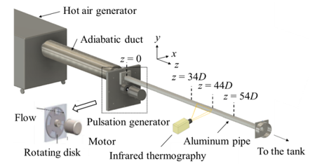
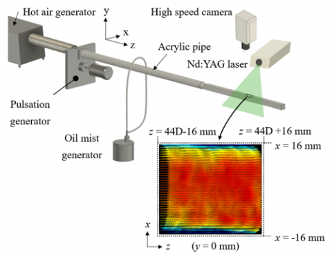
The experimental apparatus shown in Figure 1 was designed to investigate the effect of the pulsating flow in the pipe on the wall heat transfer. The working fluid of the air was heated using a hot-air generator (HAP 3100; Hakko Electric, Tokyo, Japan) and discharged through a test section into a tank at the outlet. The flow path was opened and closed by rotating a disk with holes to generate a pulsating flow, as shown in the lower left of Figure 1. The pulsation frequency was varied by controlling the rotational speed of the disk using a motor. The rectangular test pipe was made of aluminum and had a length of 2.0 m. The inner and outer hydraulic diameters were D=32 and Do=40 mm, respectively. The measurement cross-sections for temperature and velocity are located at points z=34D, 44D, and 54D from the pulsation generator to investigate the thermal-hydraulic characteristics of the developed flow.
Figure 1. Experimental apparatus
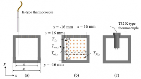
Figure 2. Measurement methods. (a) Insertion of the K-type thermocouple, (b) Measurement of the time-averaged temperature, and (c) Insertion of the T32 K-type thermocouple
The time-averaged temperature of each cross-section was measured by inserting a K-type thermocouple (T34; Okazaki, Kobe, Japan) through a hole in the upper wall of the pipe, as shown in Figure 2(a). The flow temperature was measured at 36 points per section, as shown in Figure 2(b). As shown in Figure 2(c), K-type thermocouples (T32; Anbe, Japan) consist of a 13 µm thermocouple and a 25 µm thermocouple in order to measure local temperature fluctuations. The outer wall temperature was measured using infrared thermography (890, Testo K.K., Japan), as shown in Figure 1. The cross-sectional average temperature at z/D=34 is 398 K for all conditions.
Table 2. Flow conditions
|
Rem [-] |
fp [Hz] |
Rep [-] |
Rep / Rem [-] |
Wo [-] |
|
56000 |
0 |
- |
|
- |
|
15 |
51000 |
0.91 |
33 |
|
|
25 |
62000 |
1.11 |
42 |
|
|
30 |
62000 |
1.11 |
46 |
|
|
35 |
60000 |
1.07 |
49 |
|
|
60 |
46000 |
0.82 |
65 |
|
|
90 |
23000 |
0.41 |
80 |
Table 2 lists the flow conditions used in this study. Experiments were conducted over various frequencies to simulate actual automobile engines. The flow conditions used in this study are engine exhaust flow conditions (50000<Rem<100000, Rep/Rem<1, 10<fp<100 Hz), which have been the subject of few previous studies. Two Reynolds numbers, Rep and Rem are defined for pulsating flows as dimensionless parameters based on the time-averaged velocity and amplitude, respectively.
$R e_m=\bar{w}_c D / v$, (1)
$R e_p=w_{c, p} D / v$, (2)
where, ν is the kinematic viscosity of air, $\overline{w_c}$ is the time-averaged cross-sectional average axial flow velocity, and wc,p is the amplitude of the axial flow velocity. The spatial average of wc,p from z=34D to 54D was used to define Rep. The velocity amplitude was obtained as the difference between the minimum and maximum values measured by PIV using the following equation:
$w_{c, p}=\frac{1}{2}\left(w_{c, \max }-w_{c, \min }\right)$. (3)
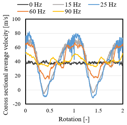
Figure 3 shows the flow velocity waveforms for two cycles at z/D=34. The horizontal and vertical axes represent the number of cycles and flow velocity, respectively. The flow velocity evidently oscillates at the pulsation frequency under all conditions, and a reverse flow with a negative velocity value appears slightly for only 15 and 25 Hz. Figure 4 shows the velocity amplitude at measurement positions 34D, 44D, and 54D and the spatial averages of the three positions. The velocity amplitude decreased as the frequency increased, except at 15 Hz, although it varied depending on the measurement position. This may be because of the fact that pulsation is generated by opening and closing the flow channel under the condition of a constant flow rate. The flow rate that flows out with one opening and one closing decrease with increasing frequency. In addition, the effect of the air column resonance is also considered insignificant because there is no peak at a specific frequency. In this study, the Womersley number is defined using the following equation, where half of the inside diameter D is the characteristic length:
$W o=\frac{D}{2} \sqrt{\frac{2 \pi f_p}{v}}$ (4)
The other experimental conditions of the ambient temperature, inlet temperature, and thermal conductivity of the pipe and air are presented in Table 3. The uncertainties of each measurement are listed in Table 4. They are defined as the standard deviation of the time-varying measurement results in steady-state flow.
Figure 3. Cross sectional average velocity (z / D = 34)
Figure 4. Velocity amplitude with respect to frequency
Table 3. Experimental conditions
|
Ambient Temperature: Tamb [K] |
Heat Conductivity of Air: λf [W/m K] |
Heat Conductivity of Aluminum: λs [W/m K] |
|
298 |
0.033 |
236 |
Table 4. Measurement uncertainties
|
Fluid Temperature at z: Ti,z [K] |
Outer Wall Temperature at z: Two,z [K] |
Cross-Sectional Average Temperature in the Pipe at z: Tfb,z [K] |
|
0.28 |
0.06 |
0.28 |
2.2 Data reduction
A schematic of the heat transfer process in a pipe is shown in Figure 5. The heat transfer from the hot air inside the pipe to the ambient fluid through the pipe wall consists of forced convection inside the pipe, heat conduction in the pipe wall, and natural convection outside the pipe. The emissivity of the pipe wall was also measured using thermography and was found to be very small (ε=0.05); consequently, the influence of radiation can be assumed to be negligible. The temporal fluctuation of the outer wall temperature is less than 0.1 K, even when measured with a high response thermography (Photron, X6901sc_SLS). This can be attributed to the higher heat capacity of the pipe material, aluminum, compared to that of air. Thus, the effect of wall temperature fluctuations can also be ignored. Therefore, the heat flux to the outside qwo,z was calculated as follows:
$q_{w o, z}=h_o\left(T_{w o, z}-T_{a m b}\right)$, (5)
where, Tamb is the ambient temperature, and Two,z is the outer wall temperature of the pipe. All temperatures used in this section are time-averaged over 10 cycles. Figure 6 shows the results of external temperature measurements. The external heat transfer coefficients ho of the left, right, upper, and lower walls were calculated from the temperature gradients at the nearest wall surface in Figure 6. Each coefficient is 14.8 (left), 15.2 (right), 6.8 (upper), and 11.4 (lower). Thus, the average value of ho=12.0 can be used as the representative heat-transfer coefficient of the pipe. Notably, the heat flux is asymmetric between the top and bottom; however, the outer wall temperatures are almost identical between the top and bottom. This is owing to the high heat conductivity of the aluminum material used in the pipe. The heat conduction equation was used to calculate the inner wall temperature: Twi,z from the local heat flux: qo,z and outer wall temperature: Two,z. As the temperature difference between Two,z and Twi,z is less than 0.1 K, the following assumptions were made.
$T_{w i, z} \approx T_{w o, z}$ (6)
Furthermore, hi,z is the local heat transfer coefficient of the inner wall of the pipe, which can be calculated using the following equation:
$h_{i, z}=\frac{q_{w i, z}}{\left(T_{f b, z}-T_{w i, z}\,\,\right)}=\frac{q_{w o, z} \;\; \alpha}{\left(T_{f b, z}-T_{w i, z}\,\,\right)}$. (7)
where, α is the cross-sectional area ratio of the outer wall to the inner wall, Tfb,z= $\sum_{\mathrm{i}=1}^{36} T_{i, z} / 36$ is the space-averaged temperature at z. α=Do/D because of the rectangular pipe. Using Eq. (7), the local Nusselt number can be defined as follows:
$N u_{i, z}=h_{i, z} \frac{D}{\lambda_f}$, (8)
where, λf is the thermal conductivity of the fluid in the pipe. The heat transfer characteristics of the pulsating flow were evaluated by calculating the local Nusselt number (Nu) inside the pipe.
Figure 5. Schematic of the tube heat transfer
Figure 6. Measurement result of temperature outside the tube at z=44D
2.3 Unsteady temperature measurement
Fluid temperature in pulsating flows is one of the most challenging and complex flow parameters to measure because of the insufficient dynamic response of temperature sensors [19]. Tagawa et al. [20] developed a reliable method to estimate the time constants of thermocouples without dynamic calibration. The method is based on a first-order delay system of two-thermocouples used to predict the actual fluctuation of the pulsating flow temperature. The actual fluid temperatures were predicted using the following two-thermocouples.
$T_{g 1}=T_1+\tau_1 \frac{\partial T_1}{\partial t}$ (9)
$T_{g 2}=T_2+\tau_2 \frac{\partial T_2}{\partial t}$ (10)
where, Tg, T, and τ are actual fluid temperature, measured temperature and time constant, respectively. Subscripts 1 and 2 denote thermocouples with diameters of 13 and 25 µm respectively. The time constants are determined when the correlation coefficient R is at its maximum.
$R=\frac{\overline{T_{g 1} T_{g 2}}}{\sqrt{T_{g 1}\,\,^2} \sqrt{T_{g 2}\,\,^2}}$ (11)
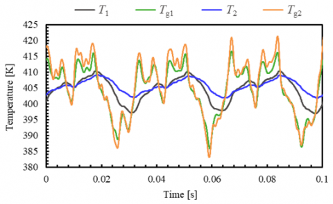
By integrating Eqs. (9) and (10) over time using the obtained time constants τ1 and τ2, the final fluid temperatures Tg1 and Tg2 can be obtained. In this study, the time constants τ1 and τ2 for the 13 and 25 µm thermocouples were 9.6 and 22.4 ms, respectively. It should be noted that Tg is identical to Tg2 for the maximum R. The details of the calculation method are provided in reference (Tagawa et al. [20]). In this method, the gain at high frequencies is extremely large because of the constant time constant, which increases the influence of noise. Therefore, a low-pass filter six times the pulsation frequency (flp=6fp) was applied for the evaluation. Figure 7 shows the results of the temperature measurements at fp=30 Hz. It can be observed that the response time delay of the thermocouple can be compensated, resulting in a larger amplitude after compensation. Because the waveforms of Tg1 and Tg2 were almost the same, Tg2 was used in this study for discussion.
Figure 7. Measurement results of pipe center temperature in pulsating flow (fp=30 Hz)
2.4 Flow field measurement
Figure 8 shows the optical system for PIV measurement to visualize the flow field on the x-z plane. The origin of the x-y coordinates was the center of the pipe. For example, the flow velocity was measured in the x-z plane at -16 mm<x<16 mm, y=0 mm, and 44D-16 mm<z<44D+16 mm, as shown in Figure 8. Oil mist with a small particle size (average particle diameter: 2-3 μm) was used as a tracer particle to ensure fluid flow trackability. A Nd:YAG laser (Continuum, Mesa PIV) was used as the light source, and particle images were acquired at 10000 fps. PIV was performed by creating pairs from these particle images under the same flow conditions as in Table 2; therefore, the time interval for the flow velocity was 5000 Hz. The x and z components of the flow velocity were calculated using the direct cross-correlation method. The PIV conditions are listed in Table 5. The inspection window was 27 pixels × 27 pixels (70% overlap). PIV based on zoomed-in images (zoom-PIV) was also conducted to evaluate the flow field near the wall surface. The conditions are listed in Table 6.
Table 5. PIV conditions
|
Frame Speed: fs [fps] |
Resolution [mm/pixel] |
Time Interval Between Laser Pulses [μs] |
Grid Size [pixel] |
Interrogation Window Size [pixel] |
|
10000 |
0.034 |
10 |
8 |
27×27 |
Table 6. Zoom-PIV conditions
|
Frame Speed: fs [fps] |
Resolution [mm/pixel] |
Time Interval Between Laser Pulses [μs] |
Grid Size [pixel] |
Interrogation Window Size [pixel] |
|
20000 |
0.0117 |
10 |
6 |
23×23 |
The cross-sectional average velocity was calculated using the following equation, where M=32 points:
$w_c(z, t)=\frac{1}{M} \sum_{i=1}^M w\left(x_i, z, t\right)$ (12)
Cross-sectional average velocities were evaluated by ordinary PIV, and the statistics presented hereafter were evaluated by Zoom-PIV. First, as proposed by Reynolds and Hussain [21], the flow characteristics can be decomposed into three terms in the case of turbulent pulsating flows, as shown in the following equation:
$w(x, z, t)=\bar{w}(x, z)+\hat{w}(x, z, t)+w^{\prime}(x, z, t)$ (13)
where, $\bar{w}(x, z)$ is the time-averaged term, $\widehat{w}(x, z, t)$ is the oscillation term, and $w^{\prime}(x, z, t)$ is the turbulent fluctuation term. The time-averaged term was obtained by taking the ensemble average of 10 cycles. The oscillatory term can be calculated using the phase-averaged process: < >.
$\hat{w}(x, z, t)=\langle w(x, z, t)\rangle-\bar{w}(x, z)$ (14)
The phase average was calculated by taking the ensemble average of 10 times with the same phase for 10 cycles of data. The turbulent fluctuations can be removed using phase averaging, and only pulsation components can be extracted from the total instantaneous profile. Eqs. (13) and (14) are used to calculate the fluctuation components $u^{\prime}(x, z, t)$ and $w^{\prime}(x, z, t)$ of the turbulence, respectively. The root mean square (RMS) value was calculated using Eq. (15) to evaluate the intensity of the turbulent fluctuations, where N is the number of data points for 10 cycles, expressed as 10×fs/2×fp.
$w_{r m s}^{\prime}(x, z)=\sqrt{\frac{1}{N} \sum_{i=1}^N w^{\prime}\left(x, z, t_i\right)^2}$ (15)
The instantaneous RMS value is calculated using the following Eq. (16) to evaluate the magnitude of w' at each pulsation phase:
$w_{r m s, p}^{\prime}(x, z, t)=\frac{1}{10} \sqrt{\left\langle w^{\prime}(x, z, t)^2\right\rangle}$ (16)
The friction velocity is calculated using the following Eq. (17) to compare the results with those of existing studies:
$w^*=\sqrt{\frac{\tau_w}{\rho}}=\sqrt{v \frac{\partial \bar{w}}{\partial x}}$ (17)
The velocity gradient normal to the wall surface in Eq. (17) is obtained by fitting a quadratic function to three points near the wall surface in the zoom-PIV results for steady flow. The value of the friction velocity w*=2.12 is obtained. To validate the value w*, the friction coefficient and wall shear stress were estimated using Eqs. (18) and (19) for turbulent flow, respectively [22]. The friction velocity obtained by Eqs. (17) to (19) was 2.03, which was in agreement with 2.12 in this study with around 4.4% difference. Therefore, the validity of the time-averaged velocity distribution measurement using PIV is confirmed.
$f=\left(1.8 \log _{10} R e-1.5\right)^{-2}$ (18)
$\tau_w=\frac{1}{8} f \rho \bar{w}_c^2$ (19)
Figure 8. Experimental apparatus for the PIV
3.1 Circumferential temperature fields in the cross-sections
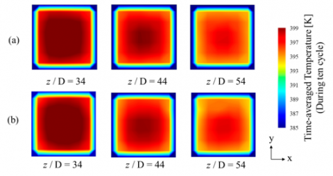
The heat transfer asymmetry was evaluated using time-averaged temperature distributions in x-y cross-section at each z. The temperature distribution was obtained from 36 temperature measurements at each cross-section, as shown in Figure 2(b). The outer wall temperature was based on the results of the thermography measurements. The color contours of the experimental temperatures were obtained using MATLAB (MathWorks, Inc., Portola Valley, CA, USA). The time-averaged temperature distribution during a 1.0 s steady flow is shown in Figure 9(a). The temperature distribution hardly deviated in all three cross-sections, and the overall temperature decreased downstream. The time-averaged temperature distribution in the pulsating flow over ten cycles at fp=30 Hz is shown in Figure 9(b). It can be suggested that symmetry is still maintained as the steady flow in Figure 9(a). These results indicate that the deviation in the y-direction that could result from buoyancy, as well as the deviation in the inlet velocity distribution that could result from the pulsation generator, can be ignored. The Richardson number is calculated as the difference between the internal fluid temperature and the wall temperature using the following equation:
$R i=\frac{g \beta_{i, z}\left(T_{f b, z}-T_{i w, z}\,\,\right) h_{i, z}}{\bar{w}^2}$ (20)
where, βi,z is the coefficient of the thermal expansion of air, which is the internal fluid in the pipe. The Richardson number varied slightly depending on the pulsation frequency and measurement location, but the maximum was approximately 0.01. This is sufficiently small to consider the forced convection to be dominant. Thus, the effect of buoyancy, which could cause the airflow velocity distribution to deviate in the pipe, is negligible.
Figure 9. Temperature distribution in tube. (a) Steady flow and (b) pulsating flow (fp = 30 Hz)
It can also be observed in the external temperature measurement results in Figure 6 that the wall surface temperature is nearly symmetrical. Therefore, the effect of heat transfer can be evaluated by the wall temperature and the representative temperature, Tfb,z.
3.2 Nusselt number evaluation
The prediction of the heat transfer coefficient in a pulsating flow is extremely difficult because heat transfer occurs with unsteady fluctuations in the flow field. This section describes the quasi-steady-state theory, which is one of the few theories on heat transfer in transient flows. In pulsating flows, a quasi-steady flow assumes that the flow behaves as if it were steady at an instantaneous rate at any time in a cycle. The most common approach to heat transfer in pulsating flows is to directly apply the quasi-steady assumption to the heat transfer correlation by substituting the absolute value of the instantaneous velocity and integrating it over one cycle. This method was first introduced by Martinelli et al. [23] and has since been used by other researchers (Hanby [2]; Ishino et al. [4]). For the Dittus-Boelter empirical correlation (Dittus and Boelter, [24]) was proposed, various correlations for steady-state heat transfer have been proposed under various conditions. Gnielinski’s equation of Eqs. (21) and (22) is adopted because of the range of Reynolds numbers (Gnielinski [25, 26]) in the present paper.
$\begin{aligned} N u_G= & \frac{(f / 8)(R e-1000) P r}{1.07+12.7 \sqrt{f / 8}\left(\operatorname{Pr}^{2 / 3}-1\right)} \\ & \text { for } 10^4<\operatorname{Re}<5 \times 10^6\end{aligned}$ (21)
$\begin{aligned} N u_G= & \frac{(f / 8) \operatorname{Re} \operatorname{Pr}}{1.07+12.7 \sqrt{f / 8}\left(\operatorname{Pr}^{2 / 3}-1\right)} \\ & \text { for } \operatorname{Re}<10^4\end{aligned}$ (22)
When Gnielinski’s equation is applied to quasi-steady turbulent heat transfer, the following equation for the Nusselt number is obtained:
$N u=\int_0^1 N u_G(R e) d \tau$ (23)
where, the Reynolds number is expressed by the following equation:
$R e=R e_m\left(1+R e_p / R e_m \cos 2 \pi \tau\right)$ (24)
where, Pr=0.72, Rem and Rep are the Prandtl number and mean flow and pulsation Reynolds numbers, respectively, as presented in Table 2, and τ is the time normalized by one cycle. The authors confirmed that the power spectrum of the velocity was maximum at each pulsation frequency in the experiment for all pulsation conditions. Therefore, the calculation of Eqs. (23) and (24) are performed, assuming that the turbulent fluctuations are sinusoidal. We have compared Eq. (23) using the experimental values.
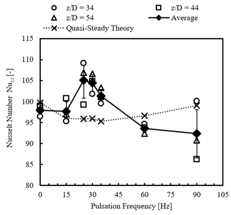
Figure 10. Nusselt number with respect to frequency
Figure 10 shows the dependence of the pulsation frequency on Nusselt numbers calculated using Eq. (8) for the present experiments at measurement positions z=34D, 44D, and 54D and their respective spatially averaged values. The quasi-steady-state theory Eq. (24) prediction is also depicted in Figure 10. The experimental result of steady flow at 0 Hz approximately agrees with the theoretical values defined in Eq. (21). Therefore, a general turbulent flow is considered to be formed in the pipe. The Nusselt number differs slightly depending on the measurement position, but this is suggested to be because of different pulsation amplitudes and temperature measurement errors. In contrast to the steady condition, the experimental results under pulsation conditions differ from the theoretical values. The result is consistent with the previous studies by Ishino et al. [4] that quasi-steady theory cannot evaluate Nusselt number very well when pulsation amplitudes are small. In addition, the evaluation of the frequency response shows that the Nusselt number has a peak at approximately 25-35 Hz. The unsteady flow field and temperature fluctuations must be evaluated to determine the cause of enhanced heat transfer at 25-35 Hz. Therefore, we measured the temperature fluctuations near the wall surface using two-thermocouple probes. Velocity fluctuations near the wall were also evaluated using zoom-PIV.
3.3 Temperature and velocity fluctuation near the wall
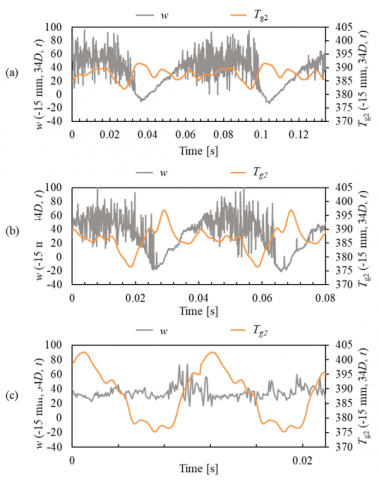
The temperature and velocity fluctuations near the wall surface were evaluated to assess unsteady thermal flow characteristics. Figure 11 shows the velocity fluctuations at 1 mm from the wall surface, as measured by PIV. The results for 15 and 25 Hz show that the velocity fluctuation increases when the velocity is high and decreases when the velocity is low. This is assumed to be due to the dominance of inertial forces over viscous forces as velocity increases. A comparison between the acceleration and deceleration phases across the maximum speed showed that the velocity fluctuation was more significant during deceleration. This could be attributed to the re-laminarization that has been confirmed in previous studies (Ishino et al. [4]) when the flow velocity is small. When re-laminarization occurs, turbulence intensity is reduced within a time delay before the flow is accelerated from laminar state to turbulent state. On the other hand, the high velocity turbulence remained during deceleration in a time delay from turbulent state to re-laminarization. The phenomena result in larger velocity fluctuations during deceleration than acceleration. Evaluation of the frequency response shows that a small velocity fluctuation is still left just before the flow velocity reaches a minimum at 25 Hz, because high turbulence remained during deceleration in the shorter time at 25 Hz than 15 Hz. The results at 90 Hz also show that velocity fluctuation increases when the velocity is high. However, the differences in the acceleration and deceleration phases, as observed at lower frequencies, could not be identified because of the small pulsation amplitude.
Figure 11 also shows the measurement results of the temperature fluctuations after correction using Eq. (10). First, the results for 15 Hz and 25 Hz show that the temperature increases when the speed is low. This can be attributed to the conversion of kinetic energy into pressure and temperature as velocity decreases. This relationship resulted in higher fluid temperatures at lower-than-average velocities. Because the wall temperature was almost constant at 383 K, a higher fluid temperature resulted in a larger difference between the wall and fluid temperatures, resulting in greater heat transfer. However, during acceleration, the intensity of turbulence was smaller owing to the rectification effect; therefore, the stirring effect was small, and the heat transfer was not very large. During deceleration, diffusion effect by turbulence and fluid temperature are high. Therefore, heat transfer enhancement is expected to occur during deceleration. At 25 Hz, the turbulence remained even at low flow velocities, resulting in a significant increase in heat transfer. This is consistent with the Nusselt number results shown in Figure 10. At 90 Hz, the temperature fluctuations were substantial; however, the intensity of turbulence was small; therefore, the heat transfer enhancement was not particularly significant. The larger temperature fluctuations at higher pulsation frequencies were assumed to be due to the faster pressure change and thus closer to adiabatic change. Therefore, the frequency characteristics of the Nusselt number shown in Figure 10 are most likely caused by turbulence and temperature changes during deceleration. The statistical process was conducted in the next section to demonstrate this correlation.
Figure 11. Time series waveforms of velocity and temperature near the wall: (a) fp=15 Hz (b) fp=25 Hz (c) fp=90 Hz
3.4 The correlation between the pulsating flow structure and wall heat transfer
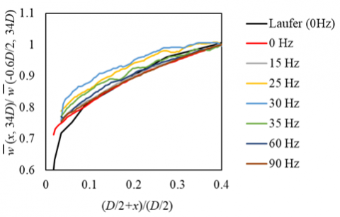
The velocity field was measured using zoom-PIV to investigate the flow structure of the pulsating flow near the wall surface. Figure 12 shows the time-averaged z-direction velocity component, which is normalized by the velocity at (D/2+x)/(D/2)=0.4, z/D=34. The horizontal axis represents the x-coordinate normalized by the length of the side of the pipe, where x = 0 is the position of the wall surface. Figure 12 shows that the velocity profiles are similar to each other, and they change sharply near the wall for all frequencies, indicating that the flow in the pipe is well-developed. An existing study (Laufer [27]) that evaluated the turbulent structure in a steady flow in a circular pipe with Rem = 50000, which is almost the same as that in the present study, is also displayed in Figure 12. It was found that a steady flow of 0 Hz agrees with Laufer, and the velocity profiles of pulsating flows are approximately the same as the steady flow.
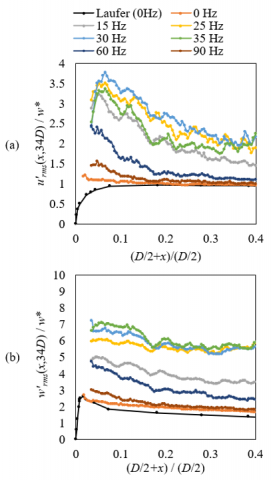
The RMS values of the turbulent fluctuations u'rms and w'rms are calculated using Eq. (15) to evaluate the effect of pulsation on the turbulence structure: The results of u'rms and w'rms are shown in Figure 13(a) and (b), respectively. We also compared the 0 Hz results of this study with those of existing studies for steady flow. It is confirmed that the RMS value of w' is almost the same as that of Laufer, and the present measurements are validated. The RMS value of u'rms is slightly different from that of Laufer, except near the wall surface, where (D/2+x)/(D/2) is less than 0.04. Although this deviation may be because of the difference between rectangular and circular pipes, the present result of u'rms is also considered to be consistent with Laufer overall. Figure 13 also shows that the RMS values differ significantly depending on the pulsation frequency. Both RMS u'rms and w'rms are large at low frequencies where the pulsation amplitude is large. The results indicate that turbulence is increased by pulsation.
Furthermore, it is found that u'rms has a peak on the x-axis between (D/2+x)/(D/2)=0 to 0.1 at 15-35 Hz, where the pulsation amplitude is large, and the value decreases from the peak to the wall surface. This peak is located at x=0.84 to 1.05 mm of actual size from the wall at 15-35 Hz. This value is close to the Stokes boundary layer thickness ($=\sqrt{v / \pi f_p}$), which is 0.7 to 0.45 mm at 15-35 Hz in the present study. Since the effect of the main flow pulsation almost disappears inside the Stokes boundary layer, the increase in turbulence owing to pulsation becomes small near the wall surface, which is suggested to have caused these peaks.
Figure 12. Time-averaged velocity at z = 34D
Figure 13. Magnitude of flow turbulent fluctuation at z=34D: (a) x-direction, (b) z-direction
Figure 14. Magnitude of turbulent fluctuation at 1 mm from the wall at z=34D. (a) x-direction, (b) z-direction
The RMS values at 1.0 mm from the wall are plotted in Figure 14 to examine the frequency response of near-wall turbulence. It can be seen that the turbulence in both x and z directions has a peak at 25-35 Hz. This result is consistent with the frequency response of the Nusselt number, as shown in Figure 10. Comparing u' and w', w' has a more similar frequency response to the Nusselt number, in that the value is smaller at 15 Hz compared at 25-35 Hz. The correlation coefficients between Nusselt number and intensity of turbulence were calculated for u' rms to be 0.47, 0.65 and 0.68 for z/D=34, 44, and 54, respectively; for w' rms, the coefficients were 0.44, 0.71 and 0.78 for z/D=34, 44, and 54, respectively. The results indicate that the Nusselt number positively correlates with both u' rms and w' rms. The larger turbulence: w'rms in the z-direction promote turbulent mixing, which in turn promotes heat transfer. The turbulence u'rms in the x-direction also has a half value of w'rms, and it directly affects the turbulent heat flux: u'T',’ which may also be the reason to enhance heat transfer in the 25-35 Hz range.
Next, the time history of the RMS value of the turbulent fluctuation in each phase is evaluated in Figure 15(a) and (b) using Eq. (16) in order to clarify the causes of increased turbulence at 25-35 Hz. The instantaneous Reynolds number is defined here as Rei=wc D/ν. According to a previous study (Laufer [27]), w'rms/w* and u'rms/w* are approximately constant for different Reynolds numbers. Therefore, we plotted the w'rms/w* and u'rms/w* for each Reynolds number using w* calculated using Eqs. (17) to (19). Figure 15 displays that the instantaneous RMS values in both w'rms/w* and u'rms/w* are larger in the phase with a higher Reynolds number, and the approximate trend is consistent with the results assuming quasi-steady value. However, hysteresis is observed during one pulsation in a pulsating flow, and the turbulence is larger during deceleration than during acceleration. This hysteresis is considered to have caused the Nusselt number to differ from that of the quasi-steady theory because the flow state in the pulsating flow is significantly different from that in the quasi-steady state. The hysteresis in the RMS values of velocity fluctuation is attributed to the small turbulence by re-laminarization during periods of small flow velocity and large turbulence during deceleration phase, especially in the case of large pulsation amplitude, as discussed in Section 3.3. Regarding the effect of pulsation frequency on the magnitude of hysteresis, the hysteresis at 25 Hz is larger than at 15 Hz because re-laminarization occurs in the deceleration phase in long time at 15 Hz, whereas in only near the minimum flow velocity because of rapid deceleration at 25 Hz. At 90 Hz, the hysteresis is very small because the pulsation amplitude is small and no re-laminarization occurs. Therefore, it is likely that turbulence during deceleration increased in the 25-35 Hz range where velocity amplitude and frequency are large, resulting in the large hysteresis in deceleration in Figure 15(a) owing to an increase in the RMS value of turbulent fluctuation. The increase is considered to have enhanced heat transfer.
Figure 15. Relationship between instantaneous Reynolds number and intensity of turbulence at 1mm from the wall. (a) x-direction, (b) z-direction
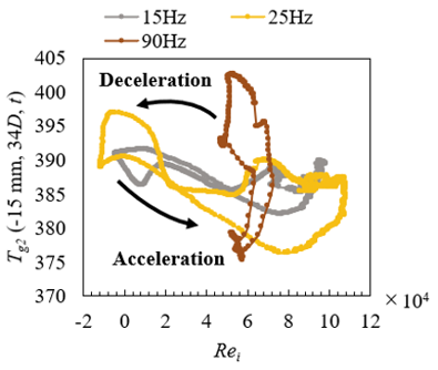
Figure 16. Relationship between instantaneous Reynolds number at pipe center and temperature at 1mm from the wall
On the other hand, focusing on acceleration phase, the flow is accelerated fast from a laminar flow state to a turbulent flow state because of short period when the frequency is high. Such a delay in turbulent transition due to fluid acceleration has been experimentally confirmed by Kurokawa and Takagi [28] and Iguchi [29]. However, the hysteresis during acceleration when the flow changes from laminar state is by far smaller than that during deceleration. Therefore, the hysteresis during acceleration is considered to have little effect on the RMS value of turbulent fluctuation and heat transfer enhancement.
Figure 16 shows that the fluid temperature is high when instantaneous Reynolds number is low except for 90 Hz. This is due to the conversion of kinetic energy into pressure and temperature as velocity decreases, as discussed in Section 3.3. A comparison at the same Reynolds number shows that the fluid temperature is higher during deceleration than acceleration. The difference between the fluid temperature and the wall temperature also increases during deceleration, and the difference is considered to have promoted heat transfer, combined with the increase in turbulence intensity mentioned above. The mechanism is considered to be another factor in promoting heat transfer by pulsation. Although the temperature difference between the fluid and the wall during deceleration is the highest at 90 Hz, heat transfer is not enhanced because the pulsation amplitude is the smallest in Figure 4 and instantaneous Reynolds number does not change very much, thus the turbulence intensity is low in this study.
As described above, the in-plane temperature distribution and wall temperature measurements showed that the heat transfer enhancement due to pulsation occurs at 25-35 Hz under engine exhaust flow conditions. Evaluation of the heat transfer characteristics under high-speed pulsating airflow conditions has been insufficient because both turbulence and temperature fluctuations have not been sufficiently measured using conventional methods. However, each of the approproiate methods such as time-resolved PIV and two-probe thermocouples to measure velocity and temperature, made it possible to find out the mechanism and characteristics of heat transfer near engine exhaust flow conditions in this study.
In this study, the frequency characteristics of convective heat transfer in a pulsating flow under engine exhaust flow conditions (Rem=56000, 15 Hz≤fp≤90 Hz) were investigated experimentally. To investigate the effect of the pulsation frequency on the heat transfer, the fluid and wall temperatures were also measured using thermocouples and infrared thermography, respectively, to evaluate the Nusselt number. Fluid temperature fluctuations near the inner wall were measured by two-thermocouple probes to evaluate unsteady-state characteristics. The flow field was measured using time-resolved PIV to elucidate the heat transfer mechanism, and the RMS value of the turbulent fluctuation was calculated. The conclusions are as follows:
This study provided the frequency characteristics of heat transfer under real engine exhaust flow conditions, where experimental data was lacking. The results deviate from the quasi-steady-state theory as in the results of Dec and Keller [3] and Ishino et al. [4], supporting the difficulty of prediction and the importance of experimental evaluation in flows with small pulsation amplitude. The heat transfer enhancement due to the pulsation in this study was not caused by resonance phenomena such as bursting [8, 10], resonance with structures [17], or gas column resonance [16], but by hysteresis of turbulence due to re-laminar flow and temperature increase during deceleration. The results in this study can help us to elucidate the mechanism of heat transfer enhancement for the design of heat transfer equipment in which resonances do not occur. The results are also expected to be used to study measures against heat loss during starting and idling of automobile engines, and to validate numerical simulations of heat transfer in pulsating flows of real automobile engines.
Editage provided editorial assistance, including English editing based on detailed instructions from the authors and organizing the references.
[1] Host, R., Moilanen, P., Fried, M., Bogi, B. (2017). Exhaust system thermal management: A process to optimize exhaust enthalpy for cold start emissions reduction. SAE Technical Paper, 1: 0141. https://doi.org/10.4271/2017-01-0141
[2] Hanby, V.I. (1969). Convective heat transfer in a gas-fired pulsating combustor. ASME Journal of Engineering for Gas Turbines and Power, 91(1): 48-52. https://doi.org/10.1115/1.3574675
[3] Dec, J.E., Keller, J.O. (1989). Pulse combustor tail-pipe heat-transfer dependence on frequency, amplitude, and mean flow rate. Combustion and Flame, 77(3-4): 359-374. https://doi.org/10.1016/0010-2180(89)90141-7
[4] Ishino, Y., Suzuki, M., Abe, T., Ohiwa, N., Yamaguchi, S. (1996). Flow and heat transfer characteristics in pulsating pipe flows (effects of pulsation on internal heat transfer in a circular pipe flow). Heat Transfer‐Japanese Research: Co-sponsored by the Society of Chemical Engineers of Japan and the Heat Transfer Division of ASME, 25(5): 323-341. https://doi.org/10.1002/(SICI)1520-6556(1996)25:5%3C323::AID-HTJ5%3E3.0.CO;2-Z
[5] Guo, Z., Sung, H.J. (1997). Analysis of the Nusselt number in pulsating pipe flow. International Journal of Heat and Mass Transfer, 40(10): 2486-2489. https://doi.org/10.1016/S0017-9310%2896%2900317-1
[6] Wang, X., Zhang, N. (2005). Numerical analysis of heat transfer in pulsating turbulent flow in a pipe. International Journal of Heat and Mass Transfer, 48(19-20): 3957-3970. https://doi.org/10.1016/j.ijheatmasstransfer.2005.04.011
[7] Zohir, A.E., Habib, M.A., Attya, A.M., Eid, A.I. (2006). An experimental investigation of heat transfer to pulsating pipe air flow with different amplitudes. Heat and Mass Transfer, 42: 625-635. https://doi.org/10.1007/s00231-005-0036-z
[8] Elshafei, E.A., Mohamed, M.S., Mansour, H., Sakr, M. (2008). Experimental study of heat transfer in pulsating turbulent flow in a pipe. International Journal of Heat and Fluid Flow, 29(4): 1029-1038. https://doi.org/10.1016/j.ijheatfluidflow.2008.03.018
[9] Elshafei, E.A.M., Mohamed, M.S., Mansour, H., Sakr, M. (2007). Numerical study of heat transfer in pulsating turbulent air flow. In 2007 International Conference on Thermal Issues in Emerging Technologies: Theory and Application Cairo, Egypt, pp. 63-70. https://doi.org/10.1109/THETA.2007.363411
[10] Habib, M.A., Attya, A.M., Said, S.A.M., Eid, A.I., Aly, A.Z. (2004). Heat transfer characteristics and Nusselt number correlation of turbulent pulsating pipe air flows. Heat and Mass Transfer, 40: 307-318. https://doi.org/10.1007/s00231-003-0456-6
[11] Habib, M.A., Attya, A.M., Eid, A.I., Aly, A.Z. (2002). Convective heat transfer characteristics of laminar pulsating pipe air flow. Heat and Mass Transfer, 38(3): 221-232. https://doi.org/10.1007/s002310100206
[12] Habib, M.A., Said, S.A.M., Al-Farayedhi, A.A., Al-Dini, S.A., Asghar, A., Gbadebo, S.A. (1999). Heat transfer characteristics of pulsated turbulent pipe flow. Heat and Mass Transfer, 34(5): 413-421. https://doi.org/10.1007/s002310050277
[13] Gbadebo, S.A., Said, S.A.M., Habib, M.A. (1999). Average Nusselt number correlation in the thermal entrance region of steady and pulsating turbulent pipe flows. Heat and Mass Transfer, 35(5): 377-381. https://doi.org/10.1007/s002310050339
[14] Patel, J.T., Attal, M.H. (2016). An experimental investigation of heat transfer characteristics of pulsating flow in pipe. International Journal of Current Engineering and Technology, 6(5): 1515-1521.
[15] Shiibara, N., Nakamura, H., Yamada, S. (2017). Unsteady characteristics of turbulent heat transfer in a circular pipe upon sudden acceleration and deceleration of flow. International Journal of Heat and Mass Transfer, 113: 490-501. https://doi.org/10.3390/en14133953
[16] Simonetti, M., Caillol, C., Higelin, P., Dumand, C., Revol, E. (2020). Experimental investigation and 1D analytical approach on convective heat transfers in engine exhaust-type turbulent pulsating flows. Applied Thermal Engineering, 165: 114548. https://doi.org/10.1016/j.applthermaleng.2019.114548
[17] Sorin, A., Bouloc, F., Bourouga, B., Anthoine, P. (2008). Experimental study of periodic heat transfer coefficient in the entrance zone of an exhaust pipe. International Journal of Thermal Sciences, 47(12): 1665-1675. https://doi.org/10.1016/j.ijthermalsci.2008.01.006
[18] Guo, G., Kamigaki, M., Inoue, Y., Nishida, K., Hongou, H., Koutoku, M., Yamamoto, R., Yokohata, H., Sumi, S., and Ogata, Y. (2021). Experimental study and conjugate heat transfer simulation of pulsating flow in straight and 90 curved square pipes. Energies, 14(13): 3953. https://doi.org/10.3390/en14133953
[19] Olczyk, A. (2008). Problems of unsteady temperature measurements in a pulsating flow of gas. Measurement Science and Technology, 19(5): 055402. https://doi.org/10.1088/0957-0233/19/5/055402
[20] Tagawa, M., Shimoji, T., Ohta, Y. (1998). A two-thermocouple probe technique for estimating thermocouple time constants in flows with combustion: In situ parameter identification of a first-order lag system. Review of Scientific Instruments, 69(9): 3370-3378. https://doi.org/10.1063/1.1149103
[21] Reynolds, W.C., Hussain, A.K.M.F. (1972). The mechanics of an organized wave in turbulent shear flow. Part 3. Theoretical models and comparisons with experiments. Journal of Fluid Mechanics, 54(2): 263-288. https://doi.org/10.1017/S0022112072000679
[22] Idel'chik, I.E. (1954). Hydraulic resistance. Mashinostroenie, Moscow, 1(4): 40-44.
[23] Martinelli, R.C., Boelter, L.M.K., Weinberg, E.B., Yakahi, S. (1943). Heat transfer to a fluid flowing periodically at low frequencies in a vertical tube. Transactions of the American Society of Mechanical Engineers, 65(7): 789-796. https://doi.org/10.1115/1.4018927
[24] Dittus, F.W., Boelter, L.M.K. (1985). Heat transfer in automobile radiators of the tubular type. International Communications in Heat and Mass Transfer, 12(1): 3-22. https://doi.org/10.1016/0735-1933(85)90003-X
[25] Gnielinski, V. (1976). New equations for heat and mass transfer in turbulent pipe and channel flow. International Chemical Engineering, 16(2): 359-367.
[26] Gnielinski, V. (2013). On heat transfer in tubes. International Journal of Heat and Mass Transfer, 63: 134-140. https://doi.org/10.1016/j.ijheatmasstransfer.2013.04.015
[27] Laufer, J. (1954). The Structure of Turbulence on Fully Developed Pipe Flow. US Government Printing Office. No. NACA-TR-1174.
[28] Kurokawa, J.I., Takagi, A. (1988). Accelerated and decelerated flows in a circular pipe (2nd report, transition of an accelerated flow. Transactions of the Japan Society of Mechanical Engineers B, 54(498): 302-307. https://doi.org/10.1299/kikaib.54.302
[29] Iguchi, M., Nishihara, K., Nakahata, Y., Knisely, C. W. (2010). Effect of initial constant acceleration on the transition to turbulence in transient circular pipe flow. Journal of Fluids Engineering, 132(11): 111203. https://doi.org/10.1115/1.4002519