ABSTRACT

The objective of this study was to demonstrate live weight estimation based on age by using Newton Interpolation method for male and female quails for seven weeks of fattening. A total of 138-day-old quail chicks were used in the study. The study demonstrated a 6th-degree polynomial interpolation for the function values obtained at seven equal intervals from 7 to 49 days. Live weight increase prediction was calculated for male and female quails between the 7th and 49th days using Newton Interpolation. Daily live weight increase for male and female quails based on observed live weights was determined. Female quails displayed more live weight increase after the 19th day compared with males. Average live weight increase in male quails was 3.81 g, and 4.63 g for females until the 49th day. The highest live weight increase was observed during the fourth week for all quails. Sum of squared errors and coefficient of determination (R²⁾ for fit of the model were calculated and the F test was performed. F, sum of squared errors, and R² obtained by Newton Interpolation for male quails and female quail were very large: 0 (approximately zero) and 0.999, respectively. The interpolation method is suitable for breeding studies.

Key Words:
error calculation; Newton interpolation; quail

Introduction

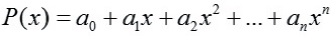
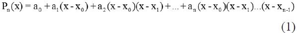
Interpolation, also known as intermediate value, is a scientific term that could be defined as arriving at an unknown intermediate value or values of a function by using known values. Interpolation is implemented within the range covered by data (Tapramaz, 2002Tapramaz, R. 2002. Sayısal analiz. Literatür Yayıncılık No: 76, İstanbul.). Different types of interpolation methods are: rational interpolation, polynomial interpolation, spline interpolation, and trigonometric interpolation (Stoer and Bulirsch, 1993Stoer, J. and Bulirsch, R. 1993. Introduction to numerical analysis. Springer-Verlag, Berlin.). The solution of several problems encountered in the field cannot be reached analytically. Generally, a given function is approximated by a class of simpler functions (Akın, 1998Akın, O. 1998. Nümerik analiz. Ankara Üniversitesi Fen Fakültesi Ders Kitapları Yayın No: 149. Ankara, Turkey (in Turkish).). A general approach for interpolation is to approximate with a polynomial of n-th degree. This polynomial is defined as follows (Xue, 2006Xue, Yi. 2006. Numerical analysis and experiment [M], publishing company of Beijing Industrial University. ):

All interpolation methods could be applied in several fields as well as to agricultural and livestock farming data. Foltyn (1991)Foltyn, J. 1991. Experience with the use of absorption reflection fensitometry on silica-gel in the analysis of Phenmedipham and Pesmedipham. Chemiche Listy 85:79-82. confirmed the method by using it for analytical definitions of desmedipham and phenmedipham in pesticide agents. It has been stated that second- and third-degree polynomial functions, y = e(a0).x(a1).x(a2(lnx)) and Lagrange interpolation methods were used on experimental data resulting in similar outcomes. Korkmaz (2009)Korkmaz, M. 2009. Deneysel verilere bazi interpolasyon yaklaşimlari üzerine bir çalişma. Doktora Tezi. Kahramanmaraş Sütçü İmam Üniversitesi, Turkey. applied Lagrange and Newton Interpolations to different data sets (cotton farming in different row spacing and intra-row distances; the effect of nitrogen dose on crop cotton plant for single stem yield; cotton plant water consumption effect; lactation milk yields in dairy cattle farming; the growth of broiler and quail; ruminant feeding; levels of protein glycosylation in human erythrocytes subjected to high glucose concentrations of capsaicin and cinnamon in vitro; and effects of fermentation length and hybrid varieties on the quality of corn silage). Interval values could be figured out by using the methods of the interpolation. Besides this statistical analysis of experimental data, additional information can be obtained by the interpolation method.

Interpolation methods can be applied in various fields. Eğecioğlu et al. (1990)Eğecioğlu, Ö.; Gallopoulos, E. and Koç, Ç. K. 1990. A parallel method for fast and practical high-order Newton interpolation. Part II Numerical Mathematics 30:268-288. examined parallel algorithms by using parallel prefix techniques to calculate divided differences in the Newton representation of the interpolating polynomial. For n +1 given input pairs, the proposed interpolation algorithm requires only 2 [log(n +1)]+2 parallel arithmetic steps, reducing the best known circuit size for parallel interpolation by a factor of logn .Sauer and Xu (1995)Sauer, T. and Xu, Y. 1995. On multivariate Lagrange interpolation. Mathematics of Computation 64:1147-1170. studied Lagrange interpolation of n-th degree of a function f, which is a sum of integrals of certain (n + l)st directional derivatives of f multiplied by simplex spline functions. Kogan and Tassa (2006)Kogan, N. and Tassa, T. 2006. Improved efficiency for revocation schemes via Newton interpolation. Journal ACM Transactions on Information and System Security (TISSEC) 9:461-486. showed that using Newton rather than Lagrange interpolants allows a significantly more efficient transmission of the new revocation message and shorter response time for each round. In a study by Zhang and Xiao (2011)Zhang, M. and Xiao, W. 2011. Construct and realization of Newton interpolation polynomial based on Matlab7. Procedia Engineering 15:3831-3835., when solution of ln(x) function, the error of quadratic polynomial of the Newton is smaller than that of linear interpolation polynomials; in this way, the interpolation error was analyzed, and the interpolation function was contrasted with the original function. Babolian et al. (2012)Babolian, E.; Hosseini, S. M. and Heydari, M. 2012. Improving homotopy perturbation method with optimal Lagrange interpolation polynomials. Ain Shams Engineering Journal 3:305-311. investigated the homotopy perturbation method (HPM) by using optimal Lagrange interpolation polynomials: HPM was successful in solving many application problems. However, difficulties could arise in dealing with determining the ui components. For that reason, modified HPM was proposed using optimal Lagrange interpolation polynomials and was applied for solving nonlinear ordinary differential equations to overcome some difficulties. Mahalik and Mohapatra (2015) Mahalik, M. K. and Mohapatra, J. 2015. A robust numerical method for singularly perturbed third order boundary value problem with layer behaviour. Procedia Engineering 127:258-262. stated that third-order singularly perturbed boundary value problem was discretized by Newton's divided difference interpolation polynomial of n-th degree on an appropriate non-uniform partition.

The objective of this study was to predict the live weight and daily live weight increase of male and female quail up to seven weeks based on age by using the interpolation method.

Material and Methods

The animal material used in this study was 138 (53 males and 85 females) Japanese quail (Coturnix coturnix japonica) provided by the poultry breeding unit of Bingol University, Faculty of Agriculture, Department of Animal Science. Birds were divided into three groups randomly, with three replicates each. Quail were identified for sex on the third week of age. During the experimental period, quail were kept in the brooder for the first week and then transferred to the multi-deck cages. The study lasted seven weeks.

Diets were designed to meet approximate needs of the quail, consisting of dry matter, energy, and other nutrients; birds were fed ad libitum with 23% crude protein and 3,100 kcal/kg metabolizable energy (ME) during the first week; 20% crude protein and 3,250 kcal/kg ME for the rest of the trial period. During the trial, the live weights of the birds were measured individually and weekly with 0.01 g precision. The diets were in pellet form and precautions were taken for the animals to have access to fresh water at all times.

A function could be considered analytical when it is a numerical function given to solve problems that could not be solved analytically but by approximating the values outside the table with the help of points given on a table numerically, or by solving the function at such points. This is achieved via function approximation and interpolation methods (Akın, 1998Akın, O. 1998. Nümerik analiz. Ankara Üniversitesi Fen Fakültesi Ders Kitapları Yayın No: 149. Ankara, Turkey (in Turkish).). The interpolation method replaces y(x) with an easily calculated function, usually a polynomial and a simple straight line. y₀, y₁,..., y_n values could be used in any polynomial formula. It has been shown that it is meaningful to use data from both sides of x interpolation point, resulting in shorter calculations (Scheid, 1988Scheid, F. 1988. Numerical analysis. McGraw-Hill Inc, New York.).

Newton Interpolation is a P(x) polynomial defined in n different points of x₀, x₁,..., x_n (Prasad, 2006Prasad, D. 2006. An introduction to numerical analysis. Norasa Publishing House, New Delhi, India.). Newton Interpolation is a polynomial of n-th degree as follows, when function values are given at (n+1) equal intervals:

Here a₀, a,..., a_n coefficients are:

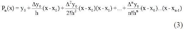
In general, at (n+1) points like x₀, x₁ = x₀ + h, x₂ = x₀ + 2h,..., x_n = x₀ + nh, the following interpolation polynomial is obtained (Turker and Can, 1997Turker, E. S. and Can, E. 1997. Bilgisayar Uygulamalı Sayısal Analiz Yöntemleri. Değişim Yayınları, Adapazarı. ):

The residue for value x (x₀ ≤ c ≤ x_n) in a interval of (x₀, x_n) the interpolation polynomial is:

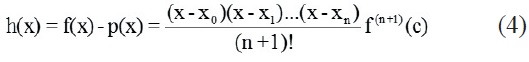
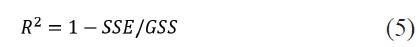
Where (x₀, x_n) = age (day) interval; c = the value (day) between x₀ and x_n; h(x) = error calculation; and f(x) = function. The goodness of a model is controlled by the goodness of fit. For this, first the sum of general squares and then the sum of error square are calculated.

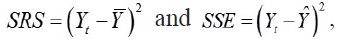
where Y_t = observation value (weight); ^_Y¯ = mean of observation (weight); and Ŷ = predicted value calculated by interpolation.

Regression sum of squares (SRS), SRS = GSS - SSE shaped. The coefficient of determination is given in equation 5:

and regression via F test was given in equation 6:

where k = parameter number; n = observation number; SSE = sum of squared errors; and GSS = general sum of squares.

Results and Discussion

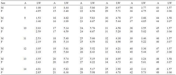
From the 7th to 49th days, quail age is the variable X in equal intervals. Corresponding live weight averages to age is the variable Y. Points have equal intervals of 7.

Live weight of male and female quail increased two-fold in the second week as compared with the first and in the third week as compared with the second (Table 1). During the first three weeks, live weight values approximated a geometric series. As of the fourth week, geometric series property disappeared. In general, female quail had a higher live weight than the male.

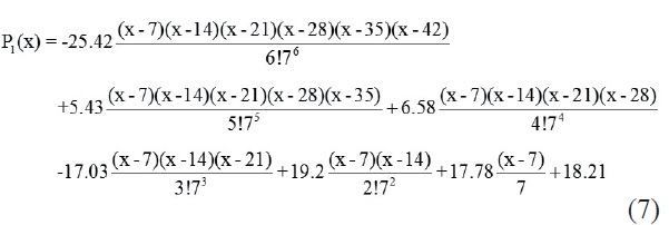
Newton Interpolation constructed to predict live weight of male quail based on age was given in equation 7:

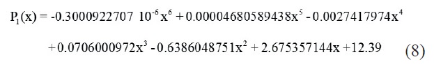
When the interpolation was regularized, the following 6-th degree polynomial was achieved (Equation 8):

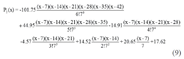
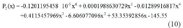
Similarly, the following Newton Interpolation was constructed to predict live weight of female quail based on age (Equation 9):

And when it was regularized, the following 6-th degree polynomial was achieved (Equation 10):

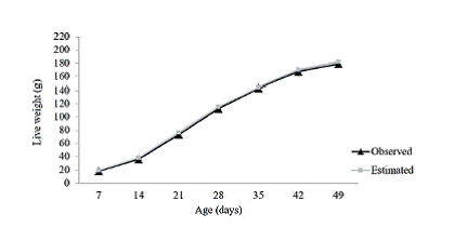
Since y values are obtained by assigning various x values in interpolation polynomials, x values of 7 to 49 days were assigned in the devised interpolations to predict live weight values (y). Graphs (Figures 1 and 2) were plotted for the determined interpolation polynomial.

Daily live weight increase in quail was determined based on the daily live weight predictions from Table 2 between days 7 and 49. Daily live weight for male quail increased by 4 kg or over after the 14th day and reached 4.01-5.86 g between days 14 and 34 (Table 2). From day 35, daily live weight increase was 1.57-3.90 g until day 49. In the 7th week (days 43-49), daily live weight increase was predicted as 1.57 and 1.58 g. The predicted daily live weight increase was 4 g or over after day 17 for female quail and determined as 4.59-6.67 g between days 17 and 42 (Table 2). In the 7th week (days 43-49), daily live weight increase was 3.06 and 3.07 g. Between days 11 and 18, live weight increase in male quail was higher than in females; after the 19th day, live weight increase was higher in females. The highest daily live weight increase was on day 22 for males (5.86 g); and on days 23 and 24 for females (6.67 g). Thus, for both for male and female quails, the highest daily weight increase was observed in the fourth week of age. Average live weight increases until the 49th day were 3.81 g for male and 4.63 for female quail. A study by Tufan et al. (2014)Tufan, T.; Arslan, C. and Sarı, M. 2014. Japon bıldırcını rasyonlarına farklı oranlarda klinoptilolit ilavesinin besi performansı, karkas verim özellikleri ve bazı kan parametrelerine etkisi. Lalahan Hayvansal Araştırma Enstitüsü Dergisi 54:1-27. reported daily average live weight increase in quale as 3.18 g between days 1 and 21; 5.01 g between days 22 and 42; and 4.10 g between days 1 and 42.

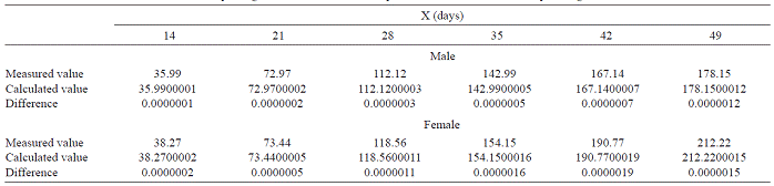
Here, "X" variable in equation was determined as an age of quails for 6^th degree Newton Interpolation (Table 3).

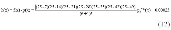
In addition to this calculation, the obtained interpolation polynomials for male and female quails at 49 days of age were P₁(x) and P₂(x) in equations 8 and 10, respectively. From these data, 6^th-degree Newton's forward-difference interpolation polynomials were achieved. According to this polynomial, real live weight of male and female quails at 14, 21, 28, 35, 42 and 49 days of age, the value of live weight calculated with P₁(x) and P₂(x) polynomial in equations 8 and 10, and differences (errors) between real measurement and calculated one were given in Table 3.

The errors with equation 4 for male quails were found as

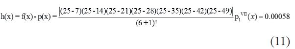
In here, p₁^VII(x) expression is the (6+1)-th differentiation of the 6th degree of interpolation polynomial. Similarly to this, error calculation for female quails is

Obtaining very low values for the differences between calculated and measured live weight indicates that the generated interpolation polynomials were suitable. If very low differences by 7-digit sensivity and a 6th-degree equation are estimated for quail live weight, it would be understood that the interpolation equation obtained with calculated errors is accurate. After obtaining these results, general sum of squares was calculated for the fit of the model (R²⁾, and the F test was performed. General sum of squares, sum of squared errors, and R² obtained by Newton Interpolation for male quails were 15444.869, 0.00000000000228831, and 0.999, respectively. The F value was found to be 6749465325939230. Significant (P<0.001) regression was very important. On the other hand, general sum of squares, sum of squared errors, and R² obtained by Newton Interpolation for female quails were 22771.493, 0.00000000000972796, and 0.999, and again, the F value was 2340829218.047770000.

According to these results, the values obtained from Newton Interpolation and the observed one were the same. Finding R² = 0.999 and a sum of squared errors = 0 (approximately zero) show the success of prediction by Newton Interpolation.

In this study, seven-week-old male quail weighed 178.15 g, and female quail, 212.22 g. Toelle et al. (1991)Toelle, V. D.; Havenstein, G. B.; Nestor, K. E. and Harvey, W. R. 1991. Genetic and phenotypic relationship in Japanese quail. Poultry Science 70:1679-1688. and Sari et al. (2010)Sari, M.; Saatci, M. and Tilki, M., 2010. Japon bıldırcınlarında (Coturnix coturnix japonica) canlı ağırlığa ait özelliklerin genetik parametrelerinin REML metodu ile hesaplanması. Kafkas Üniversitesi Veteriner Fakültesi Dergisi 16:729-733. reported by the quail at five weeks of age were found in live weight of 170 g and 176 g, respectively. Silva et al. (2013)Silva, L. P.; Ribeiro, J. C.; Crispim, A. C.; Silva, F. G.; Bonafe, C. M.; Silva, F. F. and Torres, R. A. 2013. Genetic parameters of body weight and egg traits in meat-type quail. Livestock Science 153:27-32. reported average live weight of 274.29 g in the sixth week of meat-type quail. Narinç and Aksoy (2014)Narinç, D. and Aksoy, T. 2014. Et tipi ana hatti japon bildircin sürüsünde çok özellikli seleksiyonun fenotipik ve genetik ilerlemelere etkisi. Kafkas Üniversitesi Veteriner Fakültesi Dergisi 20:231-238. indicated that the average live weight was between 174.40-178.30 g at five weeks in Japanese quail in several generations. Average live weight increases until the 49th day were 3.81 g for male and 4.63 g for female quail. A study by Tufan et al. (2014)Tufan, T.; Arslan, C. and Sarı, M. 2014. Japon bıldırcını rasyonlarına farklı oranlarda klinoptilolit ilavesinin besi performansı, karkas verim özellikleri ve bazı kan parametrelerine etkisi. Lalahan Hayvansal Araştırma Enstitüsü Dergisi 54:1-27. reported daily average live weight increase in quail as 3.18 g between days 1 and 21; 5.01 g between days 22 and 42; and 4.10 g between days 1 and 42.

Conclusions

The interpolation method is useful in animal data in terms of live weight.

References

Publication Dates

History