Abstract
The article presents a statistical physics-based model for the growth of the solid electrolyte interphase (SEI) in the negative electrode of lithium ion batteries. During battery operation, the SEI thickness grows by the reaction between lithium ions, electrons and solvent species on the surface of active particles at the negative electrode. The growth of the SEI layer causes a loss of lithium ions that induces capacity fade. In addition, it increases the ion transport resistance and decreases the total porosity. Our model employs a population balance formalism based on the Fokker-Planck Equation to describe the propagation of the particle density distribution function in the electrode. Structure-transforming processes at the level of individual particles are accounted for by using a set of kinetic and transport equations. These processes alter the particle density distribution function, and cause changes in battery performance. A parametric study of the model singles out the first moment of the initial SEI thickness distribution as the determining factor in predicting the capacity fade. The model-based treatment of experimental data allows analyzing processes that control SEI growth and extracting their controlling parameters.
Export citation and abstract BibTeX RIS

This is an open access article distributed under the terms of the Creative Commons Attribution 4.0 License (CC BY, http://creativecommons.org/licenses/by/4.0/), which permits unrestricted reuse of the work in any medium, provided the original work is properly cited.
Lithium ion batteries (LIBs) are highly touted energy storage devices for portable electronics and electric vehicles.1 The LIB system consists of a negative electrode, a positive electrode, a separator, an electrolyte, and two current collectors. The most commonly used electrolytes are comprised of lithium salts, such as LiPF6 in a solution of ethylene carbonate (EC) and dimethyl carbonate (DMC).1 The electrodes consist of randomly distributed and interconnected particles of active material, which store and release the lithium ions.
Aging and degradation of LIBs have become major concerns for the operation of electric vehicles (EVs), which must fulfill exacting requirements in terms of durability, cyclability and overall lifetime.2 Battery aging is linked to the (electro-)chemical and mechanical degradation of the electrodes and the electrolyte.2 Three main degradation mechanisms prevail at the particle level during the cycling of LIBs: (1) growth of the solid electrolyte interphase (SEI) at the negative electrode,2,3 (2) formation of cracks in the SEI layer at the negative electrode,4 and (3) dissolution and isolation of nanocrystalline particles at the positive electrode.5 These processes lead to capacity fade and power loss.
At the beginning of the battery life, particularly during the first cycle, the electrolyte undergoes reduction at the electrode/electrolyte interface, because the negative electrode operates at potentials that are outside of the electrochemical stability window of electrolyte components. This reduction is accompanied by the irreversible consumption of lithium ions.6 This process forms a passivating surface layer known as the solid electrolyte interphase. The SEI layer grows further during charging, thereby reducing the amount of active lithium ions. Moreover, this layer penetrates into the electrode pores, reducing the overall porosity and decreasing ion access to the active surface area of the electrode.2
Understanding the mechanism of SEI thickness growth and the resulting composition of the layer is a vital topic of LIB research, because of its great practical significance and the intricate interplay of underlying processes.2,6–14 The growth of the SEI involves a complex reaction network15,16 that is sensitive to operating conditions as well as the battery cycling protocol. A mechanistic understanding of the processes involved in SEI formation and growth is vital for designing LIB systems with high performance and long cycle life. The topic therefore garners significant interest in the experimental and theoretical research community.
Recent efforts in modeling of the electrochemical processes during cycling of LIBs include particle level models17,18 and porous electrode theory.16 In 1976, Bennion developed the first model of the SEI for lithium metal electrodes.19 Peled further derived a parabolic growth law for the SEI considering the electron transfer as the rate-determining step in the growth of the SEI layer.20 Ploehn et al. developed a model for SEI growth, in which the diffusion of solvent through the SEI is the rate-determining step.21 Interestingly, this assumption also leads to a parabolic growth law. Newman et al. developed a model to predict the SEI growth based on porous electrode theory, including the detailed chemistry of SEI formation.16 This model was the first attempt to link chemical reactions leading to SEI formation to irreversible capacity loss. However, it comprises a large number of model parameters. Xie et al. expanded Newman's model to incorporate thermal effects.22 They found the battery skin temperature to significantly affect the growth of the SEI. Several subsequent works are based on Newman's model. Their common feature is that they couple a one dimensional model of charge and mass transport through the electrode to a one dimensional model of spherical diffusion inside active particles, resulting in a pseudo two-dimensional porous electrode (P2D) model.23–26
Under low to moderate working conditions, the P2D model can be reduced to a single particle (SP) model.27,28 In this approach, the electrode is represented by identical spherical particles, whose accumulated surface area is equivalent to the total active area of the solid phase in the porous electrode. This model assumes that the mass and charge transport resistances in solution can be neglected. Moreover, the faradaic current across the porous electrode exhibits a linear profile, which is valid in the limit of small applied currents in thin and highly conductive electrodes.18
The modeling work presented in this article strives to establish relations among structural properties and electrochemical performance of the battery in order to rationalize the influence of SEI growth upon them. The central component of the statistical physics-based modeling framework is the Fokker-Planck Equation (FPE). The porous battery electrode is treated as a statistical distribution of interconnected particles. The FPE governs the temporal evolution of this distribution. The developed formalism allows leading causes of structural degradation, driven by (electro-)chemical and mechanical stressors, to be incorporated. Capacity and power fade as well as the battery cycle life can be analyzed in dependence of the initial structure, the external conditions and the cycling protocol applied, to predict the propagation of the particle density distribution function due to SEI growth.
Eikerling and coworkers introduced a statistical modeling framework to study the degradation of platinum nanoparticles in the cathode catalyst layer of a polymer electrolyte fuel cell.29–32 In the area of LIB research, Dreyer et al. employed a population balance approach to study the phase-change behavior of randomly dispersed interconnected particles during lithium storage.33 Röder et al. used a similar approach to study the influence of the particle size distribution on LIB performance.34
The present work aims to investigate the evolution of the SEI thickness distribution during cycling of the battery under different aging conditions. The following section introduces the statistical electrode model and it describes how the SP model for SEI growth is incorporated. Details of the numerical solution and the fitting strategy for the treatment of experimental data are given; a discussion of possible discretization schemes is provided in the Appendix. The section Results and Discussion rationalizes the dependence of capacity fade on the average SEI thickness as well as the width and tail of the SEI thickness distribution. The capabilities of the model are demonstrated by comparison to experimental data for capacity fade at varying temperature and charging rate.
Model Development
In our model, the electrodes are assumed to consist of random distributions of active particles. Particles at both electrodes are connected by inert binders. Further assumptions are that (1) the concentrations of solvent and Li ions in the solution phase are uniform, (2) the solution phase potential is uniform, (3) the electric potential in the solid phase of active particles is uniform; and (4) the faradaic current is distributed uniformly on the particle surfaces. Given these assumptions, particles charge and discharge uniformly throughout the electrode at all C-rates. The possibility of non-uniform current distribution or a particle-by-particle charging mechanism as discussed by Li et al.35 will be considered in a forthcoming work.
The transport of solvent molecules inside the SEI layer proceeds via diffusion, as shown in Fig. 1. The material balance for the solvent concentration inside of the SEI layer is
![Equation ([1])](https://content.cld.iop.org/journals/1945-7111/164/6/A1307/revision1/d0001.gif)
The boundary conditions for this equation are
![Equation ([2])](https://content.cld.iop.org/journals/1945-7111/164/6/A1307/revision1/d0002.gif)
and
![Equation ([3])](https://content.cld.iop.org/journals/1945-7111/164/6/A1307/revision1/d0003.gif)
where Ds is the diffusion coefficient for solvent molecules in the SEI layer and Cs, b is the solvent bulk concentration.
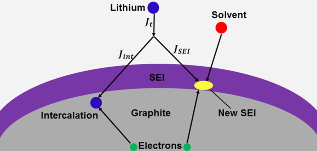
Figure 1. Parallel pathways for the transport and intercalation of Li ions into an active particle and the growth of the SEI layer through the reaction of solvent molecules with Li ions.
The diffusion of lithium ions in an active solid particle is governed by Fick's second law in spherical coordinates,
![Equation ([4])](https://content.cld.iop.org/journals/1945-7111/164/6/A1307/revision1/d0004.gif)
where C denotes the concentration of lithium ions in the particle, Di is the diffusion coefficient of Li ions in the solid and r is the radial coordinate. The boundary conditions are
![Equation ([5])](https://content.cld.iop.org/journals/1945-7111/164/6/A1307/revision1/d0005.gif)
![Equation ([6])](https://content.cld.iop.org/journals/1945-7111/164/6/A1307/revision1/d0006.gif)
For the sake of simplicity, we assume that the SEI layer grows in a reaction between Li ions, electrons and solvent molecules,
![Equation ([7])](https://content.cld.iop.org/journals/1945-7111/164/6/A1307/revision1/d0007.gif)
where Solv represents a solvent molecule such as ethylene carbonate, dimethyl carbonate, or diethyl carbonate and P stands for the reaction product.
The evolution of the SEI thickness is described by the Faraday law,
![Equation ([8])](https://content.cld.iop.org/journals/1945-7111/164/6/A1307/revision1/d0008.gif)
The SEI growth reaction is assumed to be irreversible and to follow a Tafel kinetics,
![Equation ([9])](https://content.cld.iop.org/journals/1945-7111/164/6/A1307/revision1/d0009.gif)
In this equation, kSEI is the reaction rate constant for SEI growth, Cs is the solvent concentration at the particle surface and α is the electronic charge transfer coefficient. The overpotential of SEI growth is
![Equation ([10])](https://content.cld.iop.org/journals/1945-7111/164/6/A1307/revision1/d0010.gif)
In Eq. 10, φM and φE are the potentials in metal phase and solution phase, respectively, and κSEI is the ionic conductivity of the SEI. UrefSEI is the equilibrium potential for the SEI growth, for which a value of 0.4 V vs. Li electrode has been reported.17 Jt in Eq. 10 is the total current density,
![Equation ([11])](https://content.cld.iop.org/journals/1945-7111/164/6/A1307/revision1/d0011.gif)
The electrochemical reaction for intercalation/deintercalation of Li ions at the solid/solution interface can be written as
![Equation ([12])](https://content.cld.iop.org/journals/1945-7111/164/6/A1307/revision1/d0012.gif)
where θs represents a vacant site on the particle surface.18 The rate of this reaction is given by the Butler-Volmer Equation 16,
![Equation ([13])](https://content.cld.iop.org/journals/1945-7111/164/6/A1307/revision1/d0013.gif)
where  is the intercalation reaction rate constant, Cmax the maximum solid phase concentration, Csurf the Li ion concentration at the surface of active particles and Ce the concentration of Li ions in the electrolyte, which is assumed to be constant. The overpotential for the intercalation reaction at the negative electrode, ηNint, is given by
![Equation ([14])](https://content.cld.iop.org/journals/1945-7111/164/6/A1307/revision1/d0014.gif)
Here, UN is the open circuit voltage of the negative electrode, which was extracted from experimental data of Liu et al.36 by Pinson et al.37
Population Balance Model
In this work, we employ a population balance model (PBM) based on the Fokker-Planck Equation. This approach provides a predictive framework to explore the structural evolution of a statistical distribution of solid particles, droplets, or bubbles.38 Within this framework, a random distribution of objects propagates according to the kinetics of processes that transform the properties of individual objects. The rate of these transformations of objects depends on local conditions inside the medium.39 Examples for systems described successfully by this formalism include catalyst layers of PEM fuel cells, in which the catalyst particle radius distribution changes as a result of degradation,29–32,40 biological cells in biomedical systems, e.g. in cancer research,41 or monomer droplets during suspension polymerization of vinyl chloride.42
In the mathematical formalism, the electrode is represented by a particle density distribution , which is the particle number per unit volume of the electrode in the parameter space spanned by the vector variable
  . The temporal evolution of
  is governed by the FPE,43
![Equation ([15])](https://content.cld.iop.org/journals/1945-7111/164/6/A1307/revision1/d0015.gif)
where  represents a set of quantities that describe the state of individual particles in the distribution, including for instance particle radius, SEI thickness or charging state. The drift term
  accounts for the continuous transformation of these particle properties. Source/sink terms, included in
  , represent processes that delete or add particles from or to the distribution.
The present work specifically focuses on the growth of the SEI layer thickness as the structure transforming process at the single particle level. We therefore replace  by the SEI layer thickness, δ. Moreover, it is assumed that the total number of particles is constant, which implies that source/sink terms are neglected. With these assumptions, we obtain a simplified FPE,
![Equation ([16])](https://content.cld.iop.org/journals/1945-7111/164/6/A1307/revision1/d0016.gif)
where  represents the SEI thickness change. Given an initial function f(δ, 0), Eq. 16 allows the propagation of the SEI thickness and of dependent properties to be computed. The accuracy of the calculation depends on the knowledge of f(δ, 0) and on the inclusion and suitable parameterization of particle-level processes. We consider f(δ, 0) as the distribution of the SEI thickness formed during the production of the battery; this distribution depends on the fabrication approach and conditions as well as the conditioning parameters of the battery. For the present work, we determined the initial distribution using data from SEM image analysis of a LIB negative electrode, reported in Ref. 11. These data were interpolated by an exponentially modified Gaussian (EMG) function, given by
![Equation ([17])](https://content.cld.iop.org/journals/1945-7111/164/6/A1307/revision1/d0017.gif)
with h = 0.9, μ = 32.0, σ = 8.0 and ρ = 7.5 obtained from fitting.
The solution of Eq. 16 allows for the calculation of transiently changing moments of the distribution, viz. average SEI thickness,  , and capacity fade, Qloss, as given by
![Equation ([18])](https://content.cld.iop.org/journals/1945-7111/164/6/A1307/revision1/d0018.gif)
![Equation ([19])](https://content.cld.iop.org/journals/1945-7111/164/6/A1307/revision1/d0019.gif)
![Equation ([20])](https://content.cld.iop.org/journals/1945-7111/164/6/A1307/revision1/d0020.gif)
where MSEI and ρSEI are the molar mass and the density of the SEI film and Q0 is the initial capacity of the battery.
Model Solution and Data Fitting
The system of equations is solved in MATLAB, using a central difference discretization scheme to transform the PDEs into a system of ordinary differential equations (ODEs). All ODEs are solved simultaneously employing the ode15s solver in MATLAB, which is a variable-step, variable-order solver based on the numerical differentiation formulae of order 5. Discretization of the PDEs is explained in the Appendix. Instead of time, we consider the number of cycles, N, as the independent transient variable, considering kinetic model parameters as effective parameters, i.e. average values over a single cycle.
The model was compared to capacity fade data from Wang et al. for varying T and charging rate. We adopted the same method for the capacity fade calculation as Wang et al.,44 i.e., the capacity measured during the first cycle is used as Q0. For the capacity fade simulations at different temperatures, a fitting procedure was implemented in MATLAB to find kSEI and DSolv for one set of operating conditions (15°C and C/2). A charging rate of 1C corresponds to a current of 2 A.44 At the other two temperatures (45°C and 60°C), only kSEI was fitted. For the simulation of capacity fade at different charging rates, the fitting procedure was used to obtain kSEI and Ds at 20°C and 2C. At the other two charging rates (6C, 10C), only kSEI was fitted. The list of parameters used in the simulations is presented in Table I. Parameters are based on the experimental work of Wang et al.44 and they were extracted by Prada et al.48
Table I. Model parameters used in the simulations,
| Parameter | Symbol | Value | Unit | Ref. |
|---|---|---|---|---|
| Faraday Constant | F | 96485.33 | As/mol | |
| Charge transfer coefficient | β | 0.5 | assumed | |
| SEI reaction charge transfer coefficient | α | 0.5 | assumed | |
| Universal gas constant | R | 8.314 | J/(molK) | |
| SEI layer electric conductivity | κSEI | 17.5 × 10− 5 | S/m | 48 |
| SEI layer molar mass | MSEI | 0.162 | kg/mol | 48 |
| SEI layer density | ρSEI | 1690 | kg/m3 | 48 |
| Intercalation reaction rate constant |  |
2 × 10− 6 | mol4 − 3βs− 1m1 − β | 48 |
| Maximum solid phase concentration | Cmax | 30555 | mol/m3 | 48 |
| Electrolyte concentration in solution phase | Ce | 1200 | mol/m3 | 48 |
| Active material volume fraction | εs | 0.56 | 48 | |
| Particle radius | R | 5 × 10− 6 | m | 48 |
| Solvent diffusion coefficient | Ds | 1.80 × 10− 18 | m2/s | fitted |
| SEI growth reaction rate constant | kSEI | 1.37 × 10− 17 | m/s | fitted |
| Solvent bulk concentration | CS, b | 4541 | mol/m3 | 48 |
| Diffusion coefficient of lithium ions | Di | 3 × 10− 15 | m2/s | 48 |
| Electrode surface area | A | 0.18 | m2 | 48 |
| Electrode thickness | l | 3.4 × 10− 5 | m | 48 |
Results and Discussion
Evolution of SEI layer
We first evaluated the impact of the SEI thickness growth on the single particle properties. From the initial SEI distribution (Eq. 17), we chose three sample particles with initial SEI thicknesses of 56 nm, 83 nm and 116 nm to simulate their SEI growth at 15°C and under a C/2 charging rate, as shown in Fig. 2. Initially, the SEI layer grows quickly. At higher cycle numbers, the rate of growth slows down due to the increasing ionic and diffusion resistance of the SEI layer. Since SEI thickness growth is slower for particles with initially thicker SEI layer, the three curves converge.
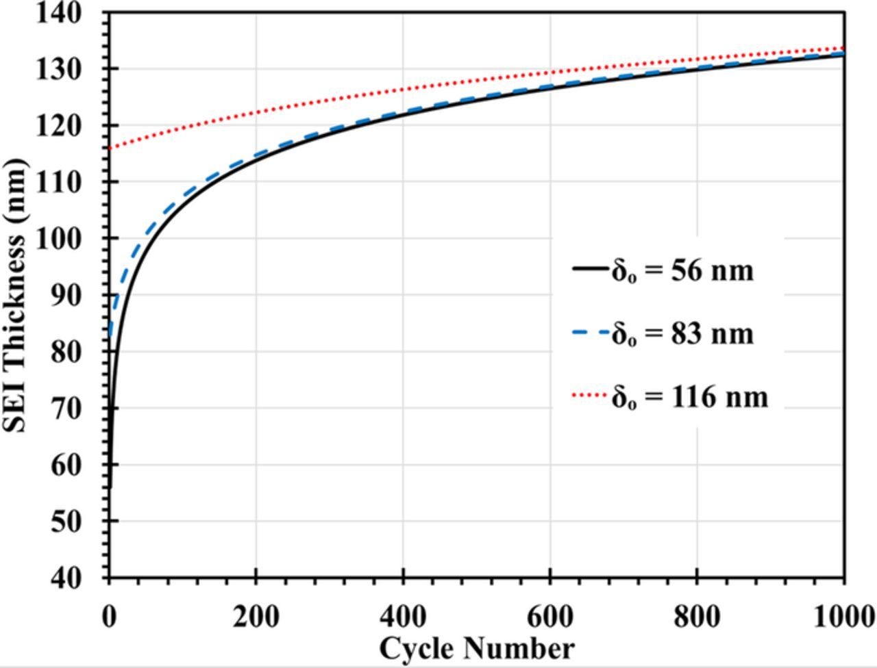
Figure 2. Growth of the SEI layer for a single particle at 15°C and C/2 charging rate.
The evolution of the SEI thickness distribution during LIB cycling is shown in Fig. 3. The overarching trend is a shift of the particle density distribution to larger average SEI thickness. Since the SEI thickness grows faster on particles with smaller initial SEI thickness, the SEI distribution narrows with N, with a corresponding increase of the height of the peak.
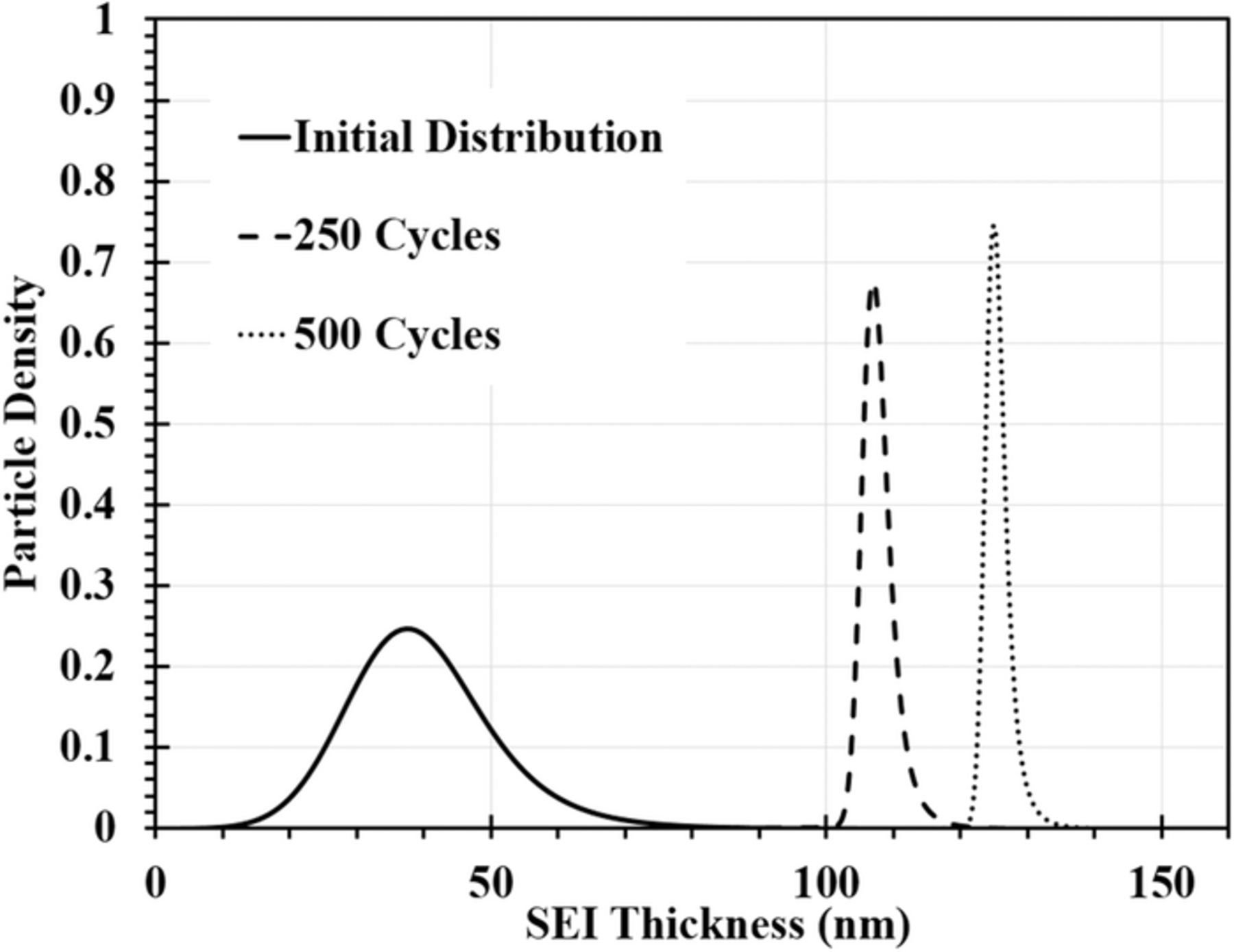
Figure 3. Evolution of the SEI thickness distribution function during cycling at 15°C and C/2 charging rate
Effect of initial SEI distribution
As explained in the modeling section, we use an EMG function (Eq. 17) to describe the initial SEI distribution. Fig. 4 shows the EMG function along with the SEM image analysis data. Three features determine the SEI distribution: (1) the average SEI thickness,  , (2) the width, (3) and the tail of the distribution. These features can be influenced during the manufacturing process and initial conditioning of the battery. We have studied the effect of each factor on the shape of the SEI distribution and on the capacity fade.
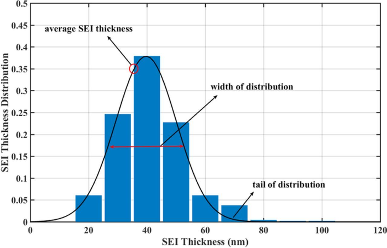
Figure 4. Initial SEI thickness distribution with SEM image analysis data.12
For comparative analyses of the impact of these characteristics, we created four initial SEI distributions, as shown in Fig. 5a: an EMG distribution as a reference case with  = 40 nm; two EMG distributions with larger
  , which were created by increasing μ from 32 to 42 and 52; an EMG distribution with the same
  as the reference case but different values of σ and ρ. The capacity fade incurred by the SEI formation that occurs during the first charge-discharge cycle of the freshly made battery and during SEI growth over 1000 subsequent cycles was simulated at 15°C and under a C/2 charging rate. The results are shown in Fig. 5b.
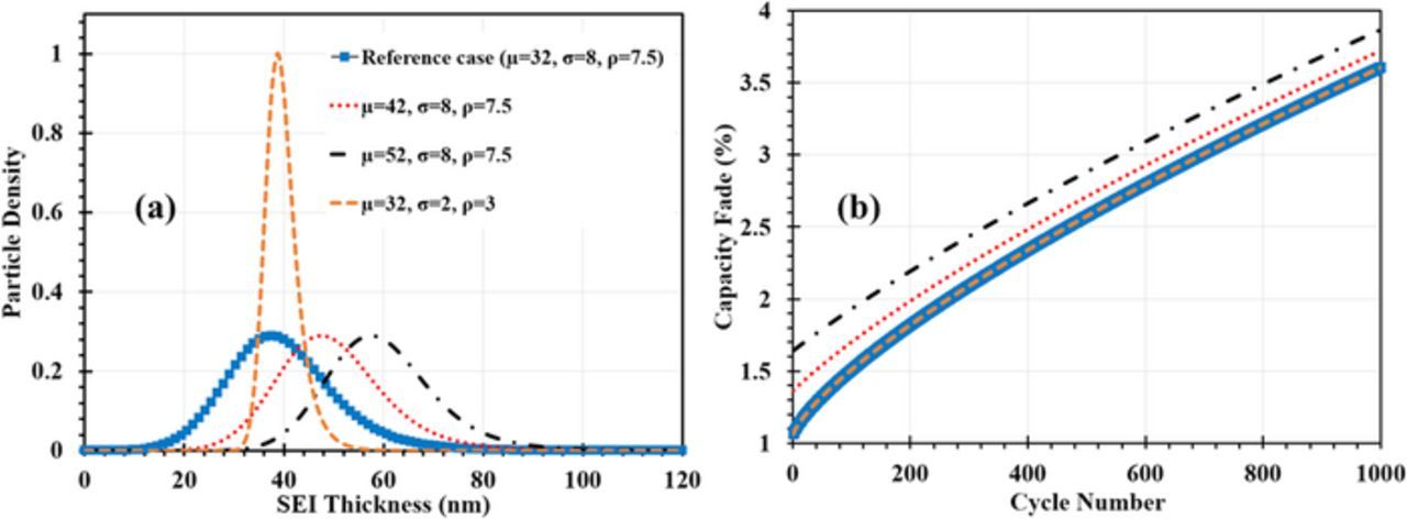
Figure 5. (a) SEI thickness distribution and (b) corresponding capacity fade including the formation stage and the cycling process.
We found that  exerts the most significant impact on Qloss, whereas the width and the tail of the particle distribution did not exert any discernible effect. This can be seen in Fig. 5b. The curves of Qloss for the two EMG distributions with
  = 40 nm but different σ and ρ lie on top of each other.
Effect of temperature on SEI thickness growth
Fig. 6 shows the result of fitting the model to experimental data for Qloss of Wang et al.44 at T = 15°C, 45°C, and 60°C in Fig. 6a and at charging rates of 2C, 6C and 10C in Fig. 6b. The fitted curves were obtained by variation of kSEI and Ds. Only the capacity fade caused by SEI growth was included for the comparison with experimental data. Higher T accelerates SEI growth due to the enhanced electrochemical reaction rate. The obtained model fits are in very good agreement with experimental data. From the Arrhenius plot in Fig. 7a and Fig. 7b we calculated an activation energy of 0.45 eV for the SEI growth reaction and 0.02 eV for solvent diffusion through the SEI layer. The activation energy of the SEI growth reaction in Eq. 7 is highly dependent on the surface properties of the negative electrode material and more importantly on the solvent properties.45 Different values have been reported in the literature, ranging from 0.34 eV to 1.5 eV.45–47 The scatter of activation energy values can be attributed to variations in cycling conditions as well as differences in materials structure and composition. For instance, we do not know what type of solvent was used by Wang et al.44
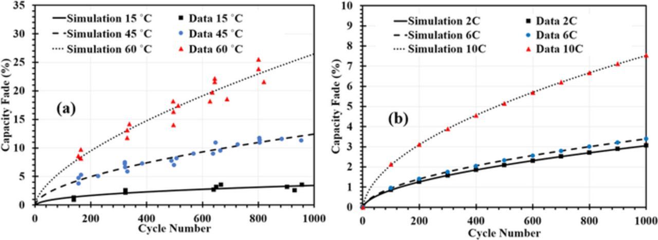
Figure 6. Capacity fade during the cycling process under (a) three different temperatures at C/2 charging rate and (b) three different charging rates at 20°C. Comparison of model with experimental data of Wang et al.44
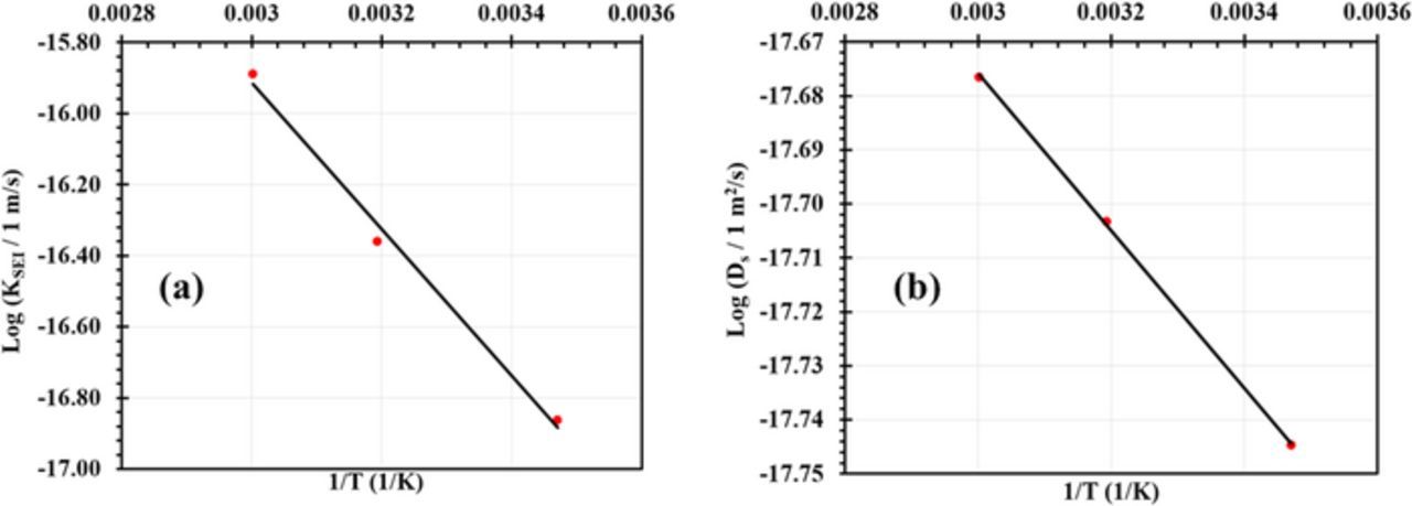
Figure 7. Arrhenius plot of (a) the SEI growth rate constant and (b) the solvent species diffusion coefficient.
Fig. 8a shows the change in the SEI thickness distribution after 100 cycles for the three curves in Fig. 6a. When T increases, the distribution shifts to higher  and the distributions becomes narrower.
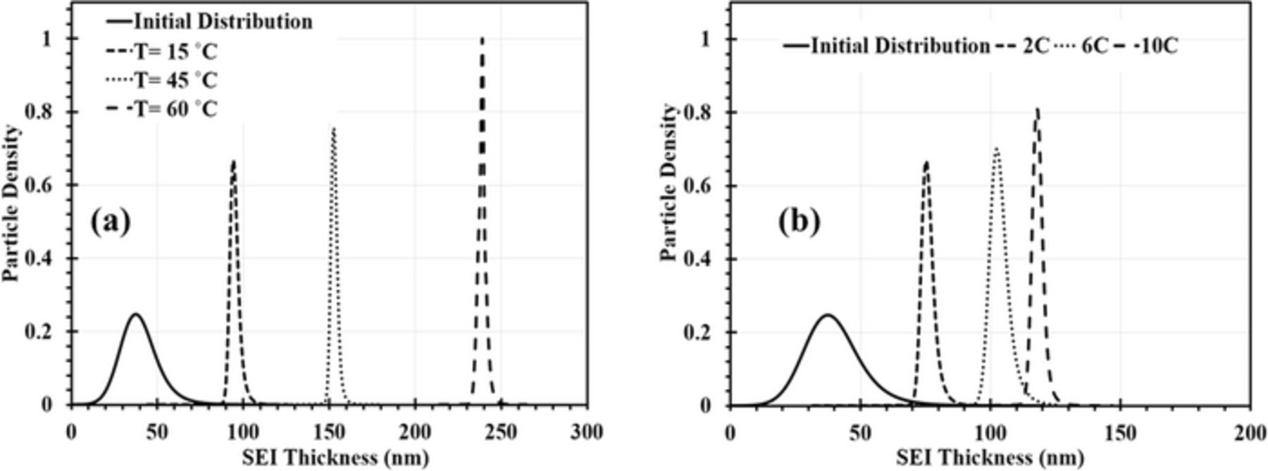
Figure 8. Evolution of the SEI thickness distribution during cycling of a LIB system at (a) three different temperatures at C/2 charging rate and (b) three different charging rates at 20°C over 100 cycles, calculated for the corresponding capacity fade curves in Fig. 6.
Effect of charging rate on SEI thickness growth
Fig. 6b reveals excellent agreement of the model fits with experimental data of Wang et al.44 for Qloss at the different C-rates. The obtained values for kSEI are 1.18 × 10− 17 m/s at 2C, 1.47 × 10− 17 m/s at 6C, and 3.59 × 10− 17 m/s at 10C. The effect of the charging rate on the change in the SEI thickness distribution after 100 cycles at 15°C is shown in Fig. 8b. By increasing the C-rate, the SEI distribution is shifted to larger  and the narrowing of the distribution, described above, becomes more pronounced.
Conclusions
This article presented a statistical physics-based model to study the impact of SEI growth on the structure and performance of the negative electrode of lithium ion batteries. The two-scale approach employs a formalism based on the Fokker-Planck Equation to relate the SEI thickness growth at the single particle level to the changes in structural properties at the electrode level. The model allows exploring the correlations of structural changes that occur during charge-discharge cycling and electrode performance.
A parametric analysis of the model reveals that the first moment of the initial SEI distribution, i.e., the average SEI thickness, is the determining factor in predicting the capacity fade. The shape and width of the initial SEI distribution do not exert any discernible impact on capacity fade. During battery cycling, the SEI thickness distribution of particle-based electrodes converges toward a narrowly shaped distribution with uniform SEI thickness.
Comparison of the model to experimental data showed convincing agreement and it allows for the rate of SEI growth and the solvent diffusion coefficient to be obtained. Further analysis using Arrhenius plots provides the activation energies of these processes. Given a set of initial structural and kinetic parameters for a specific battery electrode, the model will be able to predict the evolution of electrode structure and performance upon exposure of the battery to varying life cycle protocols. The versatile modeling framework will allow incorporating further structure-transforming processes in order to systematically improve the accuracy of that prediction.
Acknowledgments
This research was conducted as part of the project entitled "Lithium ion batteries for auxiliary power units in transportation systems: from physical modeling to optimal operation", with Cool-It HiWay Services Inc. The project is supported by the Collaborative Research and Development Grants program of the Natural Sciences and Engineering Research Council of Canada (NSERC) under file No. CRDPJ 481280 – 15. The authors wish to acknowledge discussions with Dr. Kourosh Malek, Peter Johnson and Saaed Zaeri.
: Appendix
In order to solve the Fokker-Planck equation numerically, Eq. 16 needs to be discretized. In the following, two discretization methods are discussed: constant bin sizes and growing bin sizes. With constant bin sizes, the parameter space is discretized into finite volume elements ("bins") of constant size. When the SEI on a particle grows, this particle moves from one bin into the next. In the simplest case, all elements have the same size Δδ. With this equidistant discretization and using a central difference scheme, Eq. 16 becomes
![Equation ([A1])](https://content.cld.iop.org/journals/1945-7111/164/6/A1307/revision1/d0021.gif)
where i is the index of the element. The size of each bin is given by
![Equation ([A2])](https://content.cld.iop.org/journals/1945-7111/164/6/A1307/revision1/d0022.gif)
where δmax and δmin are the largest and the smallest SEI thickness and m is the number of elements. Rinaldo et al.32 used this discretization scheme of the Fokker-Planck Equation to calculate the evolution of the Pt nanoparticle radius distribution in PEFCs. In the current model, this method is computationally more efficient for a very fine discretization of the SEI thickness distribution, e.g., when analyzing analytical distribution functions. Since the bin sizes are constant, the evolution of the solvent and Li concentration profiles during one cycle, Eqs. 1 and 4, only need to be calculated once for each bin. The SEI growth can then be assumed to happen in discrete steps after each cycle by moving the particle from one bin to the next. This way, only the Fokker-Planck Equation needs to be solved in subsequent cycles, which reduces the simulation time. A disadvantage of this method is that in order to solve the FPE accurately, a fine discretization of the SEI thickness distribution is necessary. This is often not available from experimental data, since it would require measuring a large amount of particles to get statistically meaningful results. A second problem is that only a finite parameter space from δmin to δmax is simulated. Particles leaving this parameter space are lost. Therefore, it is necessary to have a sufficient number of empty bins in stock, into which particles can move. However, it is possible to estimate an upper bound for δmax from the total amount of Li in the battery.
In the second discretization method, first the initial SEI thickness distribution is discretized. Then, the SEI growth is simulated by changing the size of the bin according to the SEI growth law, while the number of particles in each bin is constant and does not need to be calculated. This way, SEI growth is simulated by stretching the initial SEI distribution along the parameter axis. With this method, the Fokker-Planck Equation does not need to be solved explicitly, but the solvent and Li concentrations have to be updated at each time step or cycle. The computation is equivalent to solving the single particle model for each bin. This makes the method computationally inexpensive if only a few bins need to be calculated. This is usually the case for experimental data from image analysis. This second method is used in the current work.