Abstract
Micro-Raman spectroscopy was used to characterize the rust formed on 1008 carbon steel exposed to marine test sites in Hawaii. Besides lepidocrocite in the outer rust layers and goethite in the inner rust layers, akaganeite was detected on all samples due to the presence of Cl− and increased in quantity in the rust layer with increasing Cl− deposition rate. The presence of Cl− did not affect the corrosion rate of carbon steel when the Cl− deposition rate was lower than a threshold of approximately 75 mg/m2/day, but significantly increased the corrosion rate when the Cl− deposition rate was higher than the threshold. This is likely due to akaganeite being a sink for Cl− by incorporating it into its tunnel structure when salt deposition is below a certain level. Once the akaganeite is saturated with Cl− and the akaganeite cannot take up any more Cl−, free Cl− can be available to accelerate corrosion at anodic sites.
Export citation and abstract BibTeX RIS

This is an open access article distributed under the terms of the Creative Commons Attribution Non-Commercial No Derivatives 4.0 License (CC BY-NC-ND, http://creativecommons.org/licenses/by-nc-nd/4.0/), which permits non-commercial reuse, distribution, and reproduction in any medium, provided the original work is not changed in any way and is properly cited. For permission for commercial reuse, please email: oa@electrochem.org.
Marine atmosphere is one of the most corrosive environments to metallic structures due to its high content of airborne chlorides, mainly NaCl.1–5 The high corrosion rates in marine environments greatly reduce the lifetime of steel structures. Therefore, a better understanding of the corrosion mechanisms of steel is necessary for evaluating the performance and developing corrosion-control strategies.
An important aspect is to identify the various types of iron oxides and hydroxides that form on steel surfaces in various natural environments, which are believed to govern the long-term corrosion behavior. The major constituents of the corrosion products that form during atmospheric corrosion on steel are lepidocrocite (γ-FeOOH), goethite (α-FeOOH), akaganeite (β-FeOOH) and feroxyhite (δ-FeOOH),6,7 among which goethite is the most stable phase.8 Lepidocrocite is believed to form in the initial stages of atmospheric corrosion9–11 and transform to goethite in certain conditions. Akaganeite is formed only in the presence of salinity7 and was widely found in marine environments12,13 and in chloride-rich solutions14–16 and soils.17–20
Raman spectroscopy, as a powerful non-destructive spectroscopic technique, has been successfully used for the identification of pure iron oxides21–24 and steel corrosion products.8–10,12,14–20,24–30 Its ability to distinguish between the various phases of iron oxides and oxyhydroxides, which are normally found in atmospheric corrosion products, is extremely helpful in the identification of corrosion products.
In this study, Raman spectroscopy was used to identify the corrosion products that formed on steel samples which were exposed to three different marine test sites with varying levels of marine salinity ranging from 10.1 to 222.3 mg/m2/day. A layer-by-layer micro-Raman spectroscopic characterization of the rust layers was conducted. Quantitative energy dispersive X-ray analysis (EDXA) was also implemented as a complementary technique to Raman spectroscopy. The effects of the level of marine salinity on the resultant rust formation (especially that of akaganeite) and corrosion rates were elucidated.
Experimental
Sample preparation and exposure
The material used was 1008 carbon steel with chemical composition shown in Table I. The dimensions of the steel plates were 5 × 10 × 0.3 cm. The samples were attached to the exposure racks designed with a 45° angle facing the premium wind directions. The exposure racks were exposed to three locations on Oahu, Hawaii: Coconut Island (CI), Kaka'ako (KA) and Mokuleia (MO), representing various degrees of marine salinity. The corrosive ion (Cl− and SO42−) deposition rates, which were measured using dry chloride candle method,31 are shown in Table II. In each test site, a triplicate of 1008 carbon steel samples was exposed. Samples were retrieved for laboratory study after one year exposure. One sample from each test site, denoted as salinity level 1 (S1) from CI, salinity level 2 (S2) from KA, and salinity level 3 (S3) from MO was used for the present study. However, Raman analysis was conducted on all samples to verify that the results presented herein were representative of all samples.
Table I. Chemical composition (wt.%) of 1008 carbon steel.
| C | S | P | Mn | Si | Fe |
|---|---|---|---|---|---|
| 0.20 | 0.009 | 0.015 | 0.60 | 0.30 | balance |
Table II. Corrosive ion deposition rates in three test sites.
| Deposition rate (mg/m2/day) | Mild marine (CI) | Moderate marine (KA) | Severe marine (MO) |
|---|---|---|---|
| Cl− | 10.1 | 67.6 | 222.3 |
| SO42− | 2.5 | 10.6 | 43.6 |
Sample characterization
A Nicolet Almega XR dispersive Raman Spectrometer (Thermo Scientific Corp.) equipped with multiple Olympus objectives and a Peltier-cold charge-coupled device (CCD) detector was used for the experiments. Objectives with magnifications of 50× and 100×, with estimated spatial resolutions of 1.6 μm and 0.9 μm, respectively, were used. The instrument was operated with a green Nd: YAG laser with ∼532 nm wavelength excitation. The laser power was always kept lower than 1 mW to avoid sample degradation due to heating effects of the laser. The maximum spectra resolution was up to 2.2–2.6 cm−1 using 25 μm pinhole or slit, which requires longer acquisition time and reduces the signal-to-noise ratio. To reduce the collecting time, an aperture of 100 μm pinhole was used, giving an estimated resolution in the range of 8.4–10.2 cm−1. The low resolution spectra were frequently compared with high resolution spectra to prevent missing possible Raman bands. The accumulation time was 1200 seconds.
Band component analysis was realized using OMNIC spectra software (Thermo Scientific Corp.). A general spectral range from ∼200–850 cm−1 was selected for spectra deconvolution. Baseline correction was conducted using a Gaussian + Lorentzian area function before band-fitting. Squared correlation factor was maintained greater than 0.99 for all the fittings. The existence of various rust phases was first identified using the strongest bands, for example, 248, 388, and 722 cm−1 for lepidocrocite, goethite, and akaganeite, respectively. Then all bands for each phase were used for fitting.
The Raman acquisition locations were identified using adhesive copper tape markers with fine tips (D ≈ 20 μm) to facilitate the analysis of the same locations in the scanning electron microscope (SEM). A Hitachi S-3400N SEM equipped with an Oxford Instruments energy dispersive X-ray analyzer (EDXA) was used for surface morphology characterization and chemical composition analysis of the rust layers. Multiple spots were analyzed for each sample with EDXA to make sure that the results were reproducible.
Sample cleaning
After corrosion product characterization, the exposed samples, together with unexposed (virgin) control samples, were cleaned using the procedures and solutions described in ISO 8407:1991(E). Some samples required more cleaning cycles than others depending on the amount of corrosion product to be removed. Samples were considered to be clean once the mass loss between cleaning cycles was equal to, or less than, the average mass loss of virgin samples. After each cleaning cycle, samples were rinsed in deionized water, dried and then weighed in grams to four decimal places using a Mettler AE163 balance.
Results
Thick rust layers formed on all the samples that were retrieved from the three different marine test sites after one year exposure. The thickest rust layers were observed from the sample S3 at the location with the highest chloride deposition rates. The rust layers grown on the samples S1 and S2 did not show much difference in thickness by visual observation but there was a large disparity in the color of the rust. Sample S1 was dark-red on the face-up side and yellow on the face-down side, while sample S2 was dark-red on the face-up side and brown on the face-down side (Table III). Sample S3 was brown on the face-up side and with dark brown and black regions on the face-down side. The rust layers on both sides of S3 were thick. On the face-up side of S3, rust flaked off in the central region leaving the perimeters with a thicker layer of rust.
Table III. The color and composition of the rust found on the corroded samples. (L – Lepidocrocite; A – Akaganeite; G – Goethite; t – trace).
| Face-up side | Face-down side | |||||||||
|---|---|---|---|---|---|---|---|---|---|---|
| Color | Composition | Color | Composition | |||||||
| Surface | Inner | Surface | Inner | Surface | Inner | Surface | Inner | |||
| S1 | Dark-red | Black | L | G, A (t) | Yellow | Black | L | G, A (t) | ||
| S2 | Dark-red | Black | L, A | A, G | Brown | Black | A, L (t) | A, G | ||
| S3 | Brown | Black | L, A, G | A, G (t) | Dark-brown | Black | L, A, G | A, G, L (t) | ||
Raman spectra of pure iron hydroxides
Raman spectra of pure goethite and lepidocrocite from Sigma Aldrich were obtained as references and are shown in Fig. 1. The strongest bands for goethite and lepidocrocite are 387 and 248 cm−1, respectively, and can be used for the identification of these two phases.
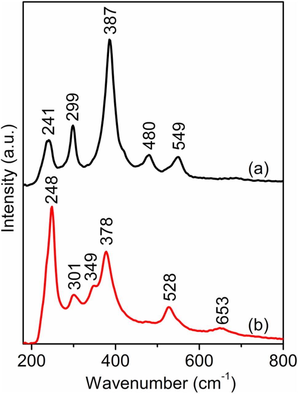
Figure 1. Raman spectra of pure (a) goethite and (b) lepidocrocite (Sigma Aldrich).
Raman spectroscopic characterization of the corrosion products
Raman spectra were obtained from both sides of the corroded steel samples. Since the samples were stored in plastic bags after being removed from the exposure racks, some rust on the sample surfaces fell off during handling, leaving some localized exfoliated regions randomly scattered on the sample surfaces. Fortunately, these exfoliated areas facilitated the acquisition of Raman spectra from the inner rust layers. In addition, surface rust layers were also manually scraped off the samples for Raman acquisition in order to confirm that exfoliated regions were representative of the inner rust layers.
Fig. 2 shows the Raman spectra from one exfoliated region on the face-up side of the sample S1, with Raman collection locations indicated in the inset. For Raman spectra representation, the original data and the fitted results are indicated by the open-circle curves and the superimposed solid lines, respectively. All band components are shown under the original data. The Raman spectrum (Fig. 2a) from the bottom of this exfoliated area shows the presence of mainly goethite since the strongest band appears at 391 cm−1 (Fig. 1a).21 However, the relatively high intensity at 248 cm−1 (compared to the band at 241 cm−1 in Fig. 1a) indicates the presence of lepidocrocite.9,10,21 Band decomposition enabled the separation of contributions from goethite which are at 241, 297, 391, 415 (shoulder (sh)), 478, 546 and 682 cm−1, those from lepidocrocite which are at 248, 335 (sh), 375, 515 and 641 cm−1 and those from akaganeite which are at 311 and 720 cm−1.18–20,28 The Raman spectrum (Fig. 2b) from the intermediate rust layer is similar to that in Fig. 2a but with higher band intensity at 251 cm−1, indicating higher lepidocrocite concentration (251, 311, 348 (sh), 378, 524 and 651 cm−1). Goethite bands are located at 241, 297, 394, 411 (sh), 481, 548 and 692 cm−1. The Raman spectrum (Fig. 2c) from the surface rust layer shows the existence of lepidocrocite with bands at 248, 305, 339 (sh), 377, 521 and 646 cm−1. The weak band at 694 cm−1 is probably due to amorphous phases in the rust layer.
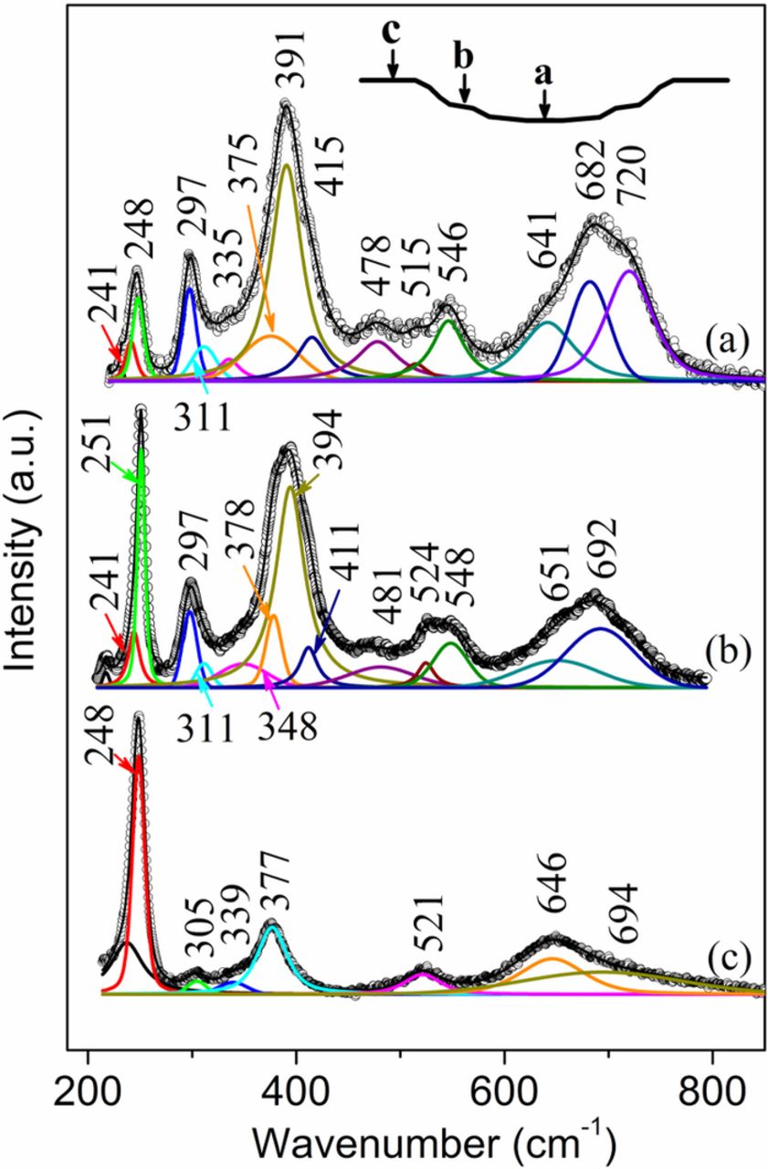
Figure 2. Raman spectra from the face-up side of the sample S1. (a) bottom of an exfoliated region; (b) intermediate rust layer; (c) surface rust layer.
Additional Raman spectra from more exfoliated regions on the face-up side of the sample S1 show similar results as shown in Fig. 2. However, large amount of akaganeite was also detected at the bottom of very few exfoliated regions (Figs. 3a and 3b) because the bands at ∼723 cm−1 are the strongest bands. Unlike the Raman spectrum shown in Fig. 2a, the Raman spectrum in Fig. 3a does not show a prominent band at ∼248 cm−1, thus excluding the presence of lepidocrocite and goethite. Hence, with the exclusion of lepidocrocite and goethite, the spectrum in Fig. 3a could likely be representative of relatively pure akaganeite that was found in all three samples. Similar to a previous study,18 band decomposition revealed 10 akaganeite bands at 268, 304, 331, 382, 419, 493, 539, 603, 688 and 723 cm−1. The Raman spectrum from another exfoliated area (Fig. 3b) shows similar akaganeite bands (302, 338, 388, 421, 466, 534, 684 and 724 cm−1) as shown in Fig. 3a but with a prominent band at 248 cm−1, indicating the presence of either goethite or lepidocrocite or both. The existence of goethite is corroborated by a relatively strong contribution at 388 cm−1. Notice that both akaganeite and goethite have contributed to most of the bands in Fig. 3b, especially those at 302, 388, 421 and 684 cm−1, since they have common Raman band positions (Figs. 1a and 3a).
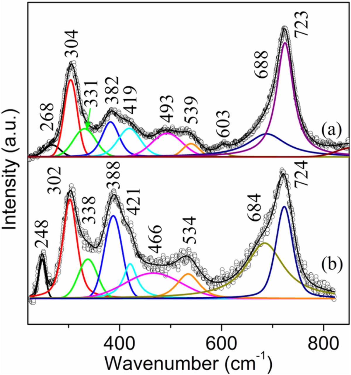
Figure 3. Raman spectra from the bottom of two exfoliated regions on the face-up side of the sample S1.
Raman spectra from the face-down side of the sample S1 showed similar results to those obtained from the face-up side: (1) lepidocrocite was found in the surface rust layer; and (2) goethite and akaganeite (scarce) were detected in the rust layers close to the substrate.
More akaganeite was detected from the sample S2 (especially the brown-colored face-down side) that was exposed to a moderate marine test site. The Raman spectra from the black rust that was revealed after scraping off the surface dark-red rust layer shows the presence of akaganeite (Figs. 4a and 4b). However, the two akaganeite spectra show different band intensity at 381/383 cm−1. The relatively high band intensity at 383 cm−1 in Fig. 4b is probably due to a small amount of goethite that coexisted with akaganeite in the inner rust layer. Another goethite band at ∼248 cm−1 is not present or noticeable because of its lower intensity compared to that of the band at 383 cm−1 (Fig. 1a). Other goethite bands, e.g., bands at 297 and 684 cm−1, are hidden under the more intensive akaganeite bands.
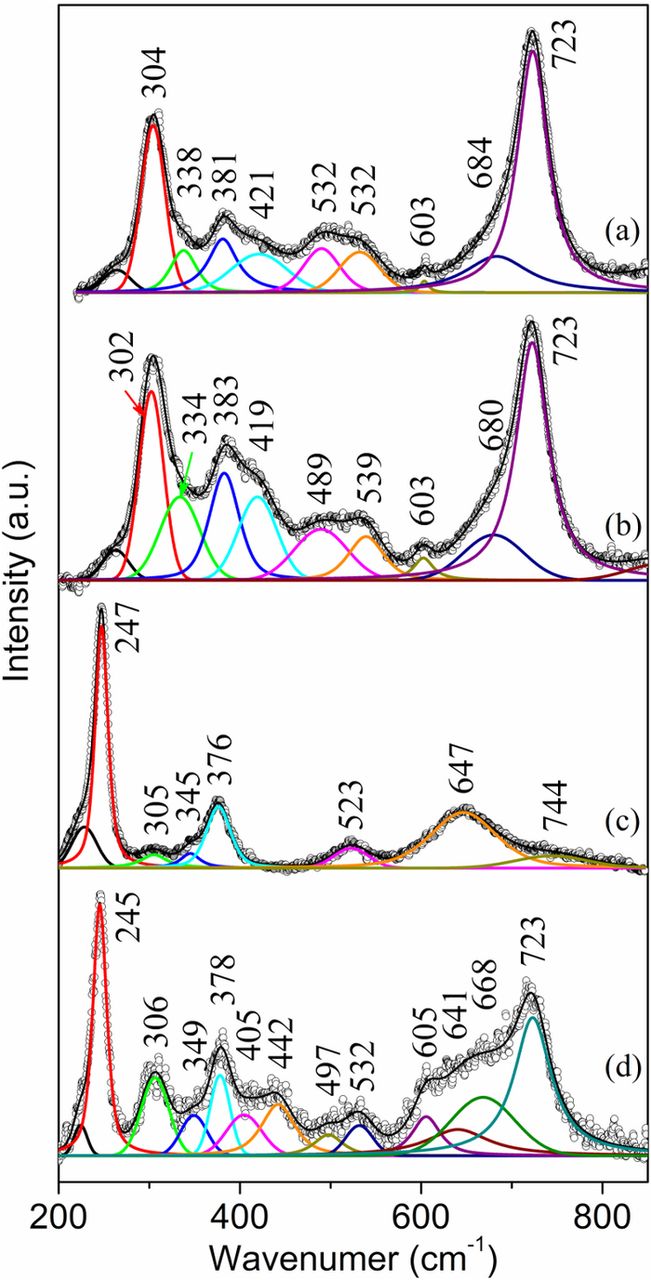
Figure 4. Raman spectra from the face-up side of the sample S2. (a) and (b) bottom of exfoliated regions; (c) surface rust layer; (d) a nodule on the surface.
The Raman spectrum (Fig. 4c) from the red surface rust layer shows the presence of mainly lepidocrocite with Raman bands at 247, 305, 345 (sh), 376, 523 and 647 cm−1. The Raman spectrum (Fig. 4d) from a brown nodule on the surface shows Raman signal of lepidocrocite (245, 349 (sh), 378 and 641 cm−1) and akaganeite (306, 405, 442, 497, 532, 605, 668 and 723 cm−1). Notice that the lepidocrocite bands at ∼306 and ∼525 cm−1 were not separated from those akaganeite bands because of their relatively low intensities.
The Raman spectra from the face-down side of the sample S2 showed the existence of akaganeite over the whole sample area (5 × 10 cm). Extensive Raman analysis was conducted on this sample and akaganeite was found to have formed at every location (over 20 locations studied) on the face-down side of this sample. In the inner rust layer, which was revealed by manually scraping off the surface layer, akaganeite was found mostly in a relatively pure form (Fig. 5a) and sometimes mixed with goethite (Fig. 5b). The Raman spectrum in Fig. 5b shows similar bands as those of pure akaganeite (Fig. 5a), but with different intensities at certain bands, especially those at 302 and 389 cm−1. Again, the relatively higher intensities at 302 and 389 cm−1 had contributions from goethite. The surface brown rust layer (Fig. 5c) also had a high content of akaganeite (304, 335, 388, 421, 494, 535 and 723 cm−1) but mixed with some lepidocrocite (245 and 374 cm−1). The presence of lepidocrocite was substantiated by the relatively strong band at 245 cm−1. Other lepidocrocite bands at ∼305, ∼343, ∼522 and ∼ 646 cm−1 were all hidden under akaganeite bands and were not revealed by band decomposition.
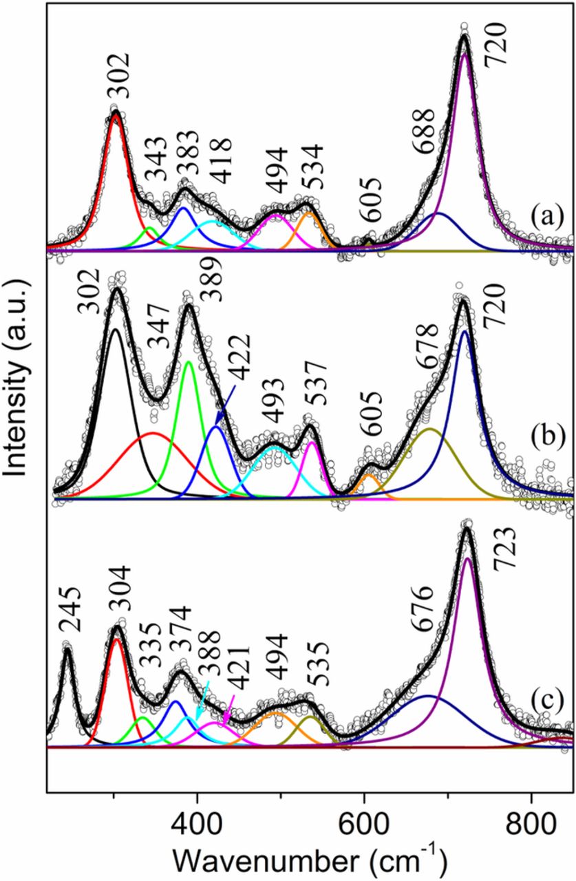
Figure 5. Raman spectra from the face-down side of the sample S2. (a) and (b) bottom of exfoliated regions; (c) a nodule on the surface.
The Raman spectrum (Fig. 6a) from the thick, compact brown rust layer that grew on the edge of the face-up side of the sample S3 shows the presence of mainly akaganeite since the band at 720 cm−1 is the strongest band. The relatively high intensity at 386 cm−1 and the existence of a band at 251 cm−1 indicate the existence of goethite. Notice that akaganeite and goethite must have both contributed to the bands at 301, 386, 410, 486, 538, and 722 cm−1. The band at 251 cm−1 might indicate the presence of a small amount of lepidocrocite since it usually exists in the surface rust layer. The Raman spectra (Figs. 6b and 6c) from the central loose rust layer show the presence of mainly lepidocrocite and akaganeite, but with different relative concentrations. The spectrum in Fig. 6b shows that the major rust component is lepidocrocite (with bands at 251, 375, 525 and 646 cm−1) since the band at 251 cm−1 is the strongest band. The second largest component is akaganeite with major bands at 301, 327, 388, 415, 486, 538, 677 and 720 cm−1. The band at 388 cm−1 being the strongest band among all the akaganeite bands indicates contribution from goethite that coexisted with lepidocrocite and akaganeite. In addition, the relatively higher band ratio of 667/720 cm−1 as compared to that in Fig. 7a may suggest the existence of magnetite (∼665 cm−1),21 which usually forms close to the metal substrate with lower oxygen availability.32,33 Another Raman spectrum (Fig. 6c) from the central loose rust region shows the presence of lepidocrocite (246, 303, 339, 381, 528 and 654 cm−1) and akaganeite (723 cm−1). The much higher band intensity at 246 cm−1 than that at 723 cm−1 suggests the predominance of lepidocrocite in some regions of the brown surface rust layer.
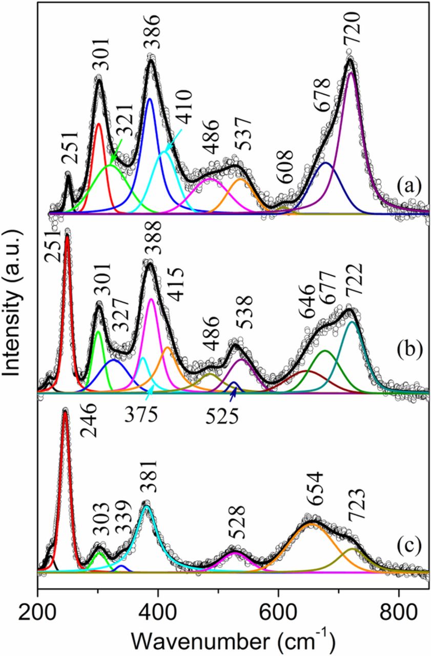
Figure 6. Raman spectra from the face-up side of the sample S3. (a) compact rust layer on the edge; (b) and (c) loose rust in the central region of the sample.
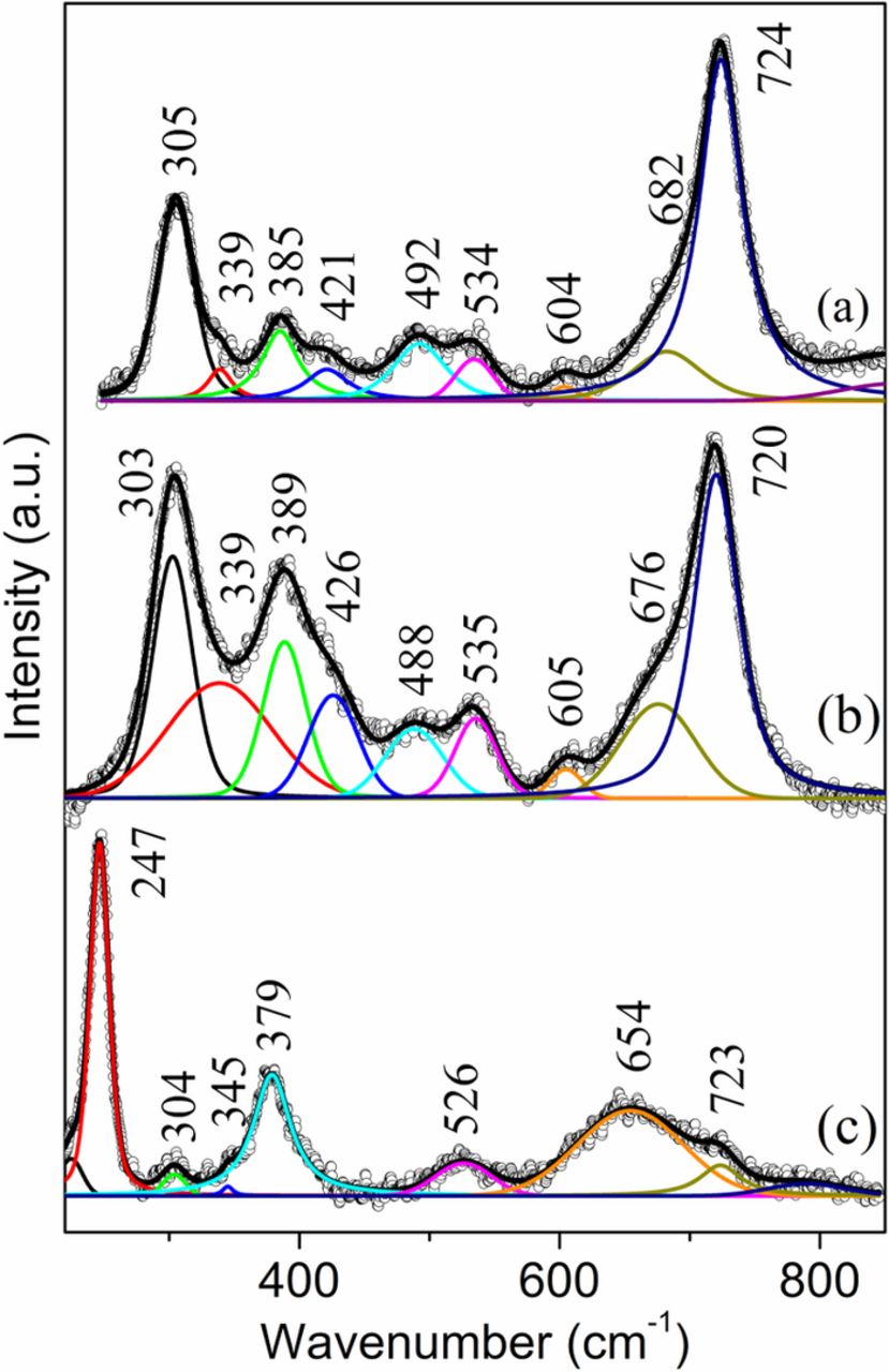
Figure 7. Raman spectra from the inner rust layer on the face-up side of the sample S3 after peeling off the thick rust layer. (a) and (b) black rust; (c) brown rust.
The Raman spectra from the face-down side of the sample S3 showed similar results as those from the face-up side of this sample with the detection of lepidocrocite and akaganeite in most locations and sometimes mixed with goethite and magnetite.
To reveal the rust close to the substrate, the thick surface rust layer was manually scraped off using a steel blade. The black rust that dominated in this inner rust layer showed a Raman signal of akaganeite either in a pure form (Fig. 7a) or mixed with goethite (Fig. 7b). Again, the presence of goethite was indicated by the much stronger band at 389 cm−1 than that (∼385 cm−1) in pure akaganeite. The Raman spectrum (Fig. 7c) from the occasionally found brown rust in the inner layer shows mainly lepidocrocite bands at 247, 304, 345, 379, 526 and 654 cm−1. A relatively weak band at 723 cm−1 is due to the presence of a trace amount of akaganeite.
The color and composition of the rust based on Raman results are summarized in Table III. Notice that the "t" (trace) marked in parenthesis indicates that the rust phase was detected in very few locations or with weak Raman signals.
SEM/EDXA characterization
Elemental quantification using EDXA was conducted at the same locations for Raman spectra acquisition. The results from the face-up side of the sample S1 indicate that the bottom of the exfoliated region had a higher Cl concentration (1.15 at.%, Table IVa), compared to 0.24 at.% (Table IVb) in the intermediate rust layer and none in the surface rust layer (Table IVc). The relatively higher Cl concentration explains the presence of akaganeite in the inner rust layer. Additional quantitative EDXA results from the locations where akaganeite was detected all showed Cl concentration in the range of 2–4 at.%.
Table IV. Elemental compositions (at.%) of rust.
| O | S | Cl | Mn | Fe | |
|---|---|---|---|---|---|
| a | 74.94 | 0.44 | 1.15 | - | 23.47 |
| b | 70.67 | 0.38 | 0.24 | - | 28.72 |
| c | 69.93 | 0.21 | - | - | 29.86 |
| d | 71.66 | 0.18 | 2.13 | - | 26.07 |
| e | 30.44 | - | 45.56 | 0.24 | 23.76 |
| f | 70.30 | 0.50 | 7.54 | - | 21.65 |
The quantitative EDXA results from most locations in the surface rust layer on the face-up side of sample S2 showed a small amount or the absence of Cl, similar as the results from the sample S1. However, in scattered locations with rust nodules (Fig. 8a), a relatively high Cl concentration was detected (2.13 at.%) (Table IVd), which corroborates the existence of akaganeite detected using Raman spectroscopy (Fig. 5c). The akaganeite-containing rust had many cracks (Fig. 8a) but looked compact under high magnification (Fig. 8b).
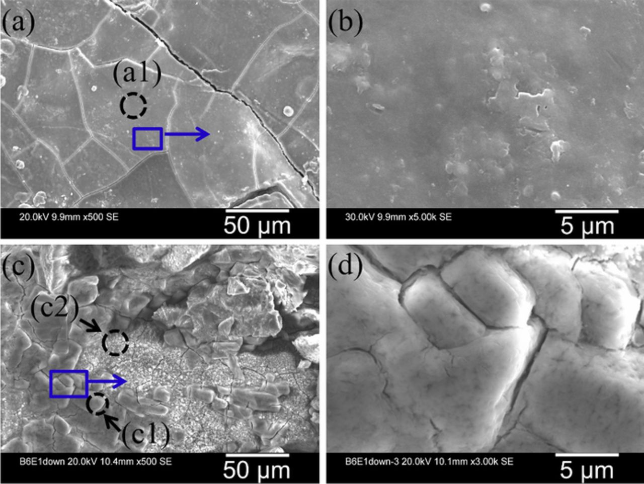
Figure 8. (a) and (b) SEM images from the rust nodules (akaganeite) found in the surface rust layer on the face-up side of the sample S2; (c) and (d) SEM images of the akaganeite found in the inner rust layer on the face-down side of the sample S2.
The EDXA result from one location in an exfoliated region (c1 in Fig. 8c) on the face-down side of the sample S2 shows a very high Cl concentration of 45.56 at.% (Table IVe). Another location in this exfoliated region also showed a high Cl content of 7.54 at.% (c2 in Fig. 8c, Table IVf). Both Cl-concentrated regions were identified as akaganeite, with Raman spectra similar to that shown in Fig. 5a.
The EDXA results from the porous rust layer on the face-up side of the sample S3 showed less amount of Cl (< 1 at.%), similar as those shown in Table IVb. The relatively low concentration of Cl agrees well with the Raman results shown in Figs. 6b and 6c which indicated the presence of mainly lepidocrocite. The rust on the edge of the face-up side of the sample S3 showed a Cl concentration of 2–4 at.% and was identified as mainly akaganeite and goethite (Fig. 6a). The EDXA results from the inner rust layer on the face-up side of the sample S3 showed relatively higher concentration of Cl in the range of 2–10 at.%, with black rust layer (akaganeite) corresponding to higher Cl concentrations, and brown rust (lepidocrocite) corresponding to lower Cl concentrations.
Discussion
The formation of akaganeite in marine environments
There is a general agreement on the predominance of lepidocrocite and goethite in the rust composition for atmospheric corrosion of steel. Among the two rust phases, lepidocrocite is usually the first oxyhydroxide that forms from corrosion.9,10,34,35 As corrosion proceeds inside towards the steel substrate, goethite tends to form from lepidocrocite transformation.32,36,37 Therefore, lepidocrocite is always found on the surface while goethite only exists in the inner rust layer near the steel substrate (Fig. 9).8,27 The findings in the present work corroborate previous results in the literature. Besides lepidocrocite and goethite, akaganeite is another prevalent rust phase found on samples from marine environments.
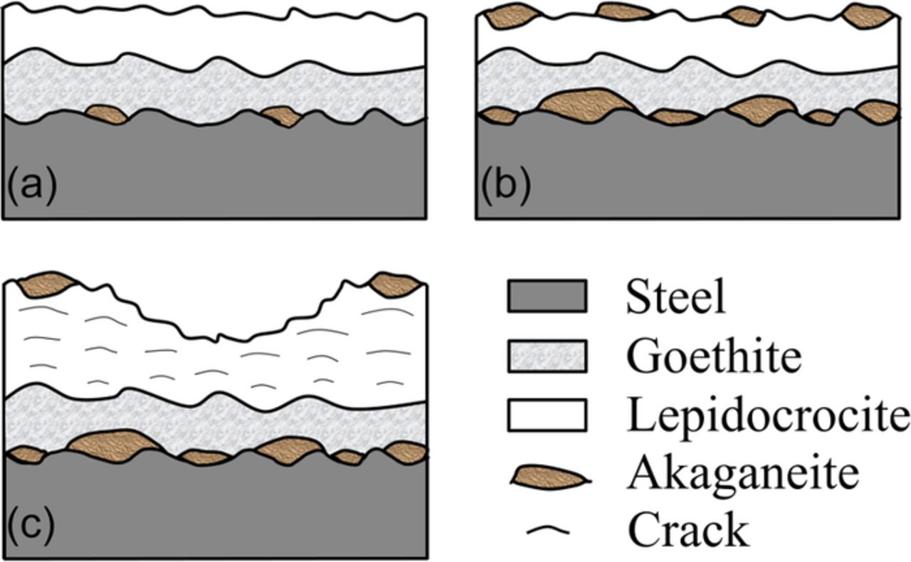
Figure 9. Schematic diagrams showing the approximate distribution of various rust phases in samples (a) S1; (b) S2; and (c) S3.
Akaganeite is known as a typical corrosion product that forms on steel samples exposed to marine environments with high chlorinity because the formation of akaganeite requires halogen ions such as Cl− which stabilize the tunnel structure of akaganeite crystals.38,39 It is believed that akaganeite comes from the oxidation of green rust GR1(Cl),40–42 which is one of the initial rust phases in NaCl-induced marine atmospheric corrosion.9,10 Sea salts that deposit on steel samples first initiate corrosion and then can be incorporated into the corrosion products.43 Sea salt crystals that are not incorporated into the corrosion products can be subsequently rinsed off by rain, depleting Cl− from the sample surface. With continued out-door exposure, however, the sample can become replenished with Cl− by newly-deposited sea salt. When the sample surface is wet, corrosion can take place under the rust layer at the steel substrate generating excess positive charge (i.e., Fe2+ and H+ from hydrated Fe ions). To maintain charge neutrality, anions such as Cl− need migrate to the corroding substrate. The migration of Cl− ions is also facilitated by the high permeability of Cl− in the rust layer,34,44 and the enrichment of Cl− into the rust/substrate interface is a direct result of this migration to maintain charge neutrality.45,46 The Cl− ions can also migrate more easily towards the steel substrate if there are cracks in the rust layer.47 The high concentration of Cl− in the inner rust layer will facilitate the formation of akaganeite.40
The distribution of akaganeite
On the sample S1 from the mild marine environment (Cl− deposition ≈10.1 mg/m2/day), akaganeite was sporadically detected primarily in the inner rust layer (Fig. 9a), and coexisting with lepidocrocite (Fig. 4d) in trace amounts on the surface. The relatively low chloride deposition rate (Table II) at the mild marine environment would have limited the amount of chloride that could have been incorporated in the rust products. Therefore, only a small amount of akaganeite was detected in the inner rust layer. More akaganeite was found on the sample S2 (Cl− deposition ≈67.6 mg/m2/day). On the face-up side, akaganeite (Figs. 4a and 4b) was detected mostly near the steel substrate due to the accumulation of Cl− ions (Table IVe and IVf) by migration to the rust/substrate interface from the surface-deposited sea salts. A considerable amount of akaganeite also formed on the surface in forms of rust nodules (Fig. 9b), as reported in the literature.45,46 The existence of akaganeite on the sample surface is related to the relatively high chloride deposition rate of 67.6 mg/m2/day (Table II), which resulted in a large amount of sea salts deposited on the sample surface. More akaganeite formed on the face-down side (as compared to the face-up side) of the sample S2 due to higher amounts of salt accumulation (Table IVe and IVf), which was likely the result of minimal salt wash off caused by rain. On the face-up side of the sample S3 (Cl− deposition ≈222.3 mg/m2/day) from the severe marine test site, more akaganeite was detected in the inner rust layer due to a higher Cl− deposition rate as compared to that for the sample S2. However, less akaganeite was detected on the outer layers of the face-up side of the sample S3 as compared to that on the sample S2, which was likely due to rust spallation of the outer layers on the heavily corroded S3 sample (Fig. 9c). Notice that relatively a large amount of akaganeite exists on the edge of the face-up side of the sample S3 where not much rust spalled off this sample (Fig. 9c). Compared to the akaganeite layer on sample S2, a similar akaganeite layer should have formed on sample S3 much earlier than on S2 due to the significantly higher chloride deposition rate at the severe marine (S3) test site compared to the moderate marine (S2) site (Table II). It is believed, therefore, that significant amounts of akaganeite had initially formed on the S3-sample surface during exposure, but much was lost by spallation of corrosion products from the outer layers and with the possible transformation to other oxides due to weathering.
Once a relatively pure akaganeite layer formed, excess Cl− cannot be incorporated into the structure and no more akaganeite can form. However, if rain leaches Cl− from the akaganeite, it can be transformed back into other forms of iron oxides. Progressive washing can remove Cl− from akaganeite,18,39,48 but the extent of removal has not been fully resolved. Some studies have suggested that washing removes Cl− ions adsorbed on the surface of akaganeite particles instead of the Cl− ions from the tunnels of akaganeite.49,50 Reguer et al.51 found that Cl− adsorbed on the akaganeite surface can be easily removed by rinsing in pure water, and that less than 1% of Cl− can be leached from the tunnel structure by extensive rinsing (with repetitive steps, 72-hr per step). Other studies have estimated that most of the Cl− ions released by washing are from tunnel sites and only 13% are from surface sites.52 It has also been reported that it is extremely difficult to completely remove Cl− ions from akaganeite, and that extensive washing could result in structural Cl− deficient in akaganeite.53–55 It is also widely believed that a minimum content of Cl− is required to stabilize the akaganeite structure, and the removal of the Cl− ions from akaganeite will induce the transformation of akaganeite to other iron oxide/oxyhydroxide phases, such as goethite or hematite depending on the pH.56 In this study, since only lepidocrocite was detected on the central surface of the sample S3 (face-up side), it is believed that akaganeite or any transformed phases (e.g., goethite) had spalled from the central surface of the sample S3. The disappearance of akaganeite after long periods of outdoor exposure was also reported.57
The Cl content in akaganeite
The Cl content in akaganeite, both synthetic and naturally formed on steel, have been determined experimentally but varied significantly depending on the formation conditions. A list of the akaganeite samples from literature is given in Table V. The synthetic akaganeite powders, made from the hydrolysis of ferric chloride solution, contain up to 12.0 wt.% of Cl.18,51 Akaganeite samples with less Cl (4.5–10 wt.%) were obtained by successive washing the synthetic powders in pure water to leach some of the Cl. The akaganeite sample on archeological iron were found to contain up to 8.0 wt.% Cl,18–20 less than the maximum Cl content in synthetic akaganeite which is 12.0 wt.%, possibly due to the relatively low Cl concentration in the soils to which the samples were exposed. However, the akaganeite formed on carbon steel exposed to a tropical marine environment contained Cl in concentrations as high as 33 wt.%.44 Similarly, in the present study, we found akaganeite with extremely high Cl contents (45.6 at.% or 46.9 wt.%) on carbon steel exposed to Hawaii's tropical marine environments. Theoretically, the Cl content in akaganeite is only approximately 6.24 wt.% according to Ståhl et al.50 Assuming that the 6.24 wt.% of Cl is embedded in the structure channels of akaganeite, the excessive Cl that was detected in the cases discussed above is believed to be adsorbed on particle surfaces and can be removed by washing. The amount of Cl that can be adsorbed on akaganeite particles is still open to investigation.
Table V. The Cl contents in various akaganeite samples from literature.
| Types of sample | Cl contents | References |
|---|---|---|
| Synthetic | 2.3–6.4 wt.% | 59 |
| 4.5–12.0 wt.% | 51 | |
| 4.5–12.0 wt.% | 18 | |
| Archaeological iron | 1.0–4.0 wt.% | 20 |
| 5.0–8.0 wt.% | 19 | |
| 8.0 wt.% | 18 | |
| Road de-icing salt environment | 1.5 wt.% | 60 |
| Marine atmospheric environment | 33.33 wt.% | 44 |
The effect of akaganeite on the corrosion of carbon steel
The corrosion rates of 1008 carbon steel in the three marine test sites are compared in Fig. 10. In addition to the three samples in the present study, additional data points from other Hawaii sites are presented in Fig. 10.58 The hockey-stick shape curve (Fig. 10) indicated that the corrosion rates were not significantly affected by Cl− deposition rates lower than approximately 75 mg/m2/day at the Hawaii sites; whereas, the formation of akaganeite was dependent on Cl− deposition rates. As discussed in above sections, significantly more akaganeite formed on the sample exposed in the moderate marine test (Cl− deposition ≈ 67.6 mg/m2/day) compared to the mild marine test site (Cl− deposition ≈ 10.1 mg/m2/day) (Fig. 9). This indicated that the formation of akaganeite did not increase the corrosion rate of carbon steel (from S1 to S2), and, therefore, akaganeite itself does not pose a threat to steel, as espoused earlier by Ståhl et al.50 who concluded that "akaganeite is itself not a problem, but rather a symptom of a problem".
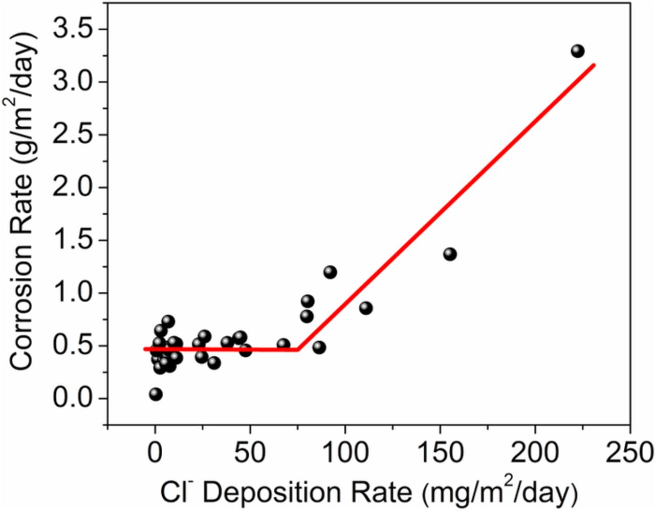
Figure 10. The corrosion rates of the 1008 carbon steels samples for one-year exposure at various Hawaii test sites.58
The above observations indicate when salt deposition is below a certain level (depending on the environmental conditions) akaganeite acts as a sink for Cl− by incorporating it into its tunnel structure. This may reduce the accumulation of Cl− directly on the steel surface and attenuate the dependency of the corrosion rate on the Cl− deposition rate. The Cl− bound in the akaganeite tunnel structure is likely difficult to remove. Once a significant amount of corrosion products at the steel interface is converted to akaganeite, free Cl− can become available in those regions after the akaganeite cannot take up any more Cl− in its tunnel structure. When the Cl− concentration is high, excess Cl− can adsorb and desorb on the akaganeite surface. Hence, when the Cl− deposition rate is above the threshold, free Cl− can be available to accelerate corrosion at anodic sites. The high levels of Cl− may also induced cracking in the rust layer through volume expansion, allowing more free Cl− ions to migrate to anodic sites and induce corrosion. As a result, it is likely that the dependency of corrosion rate on Cl− deposition rates will become evident at sites only when Cl− deposition is above the threshold, as observed at test sites in Hawaii (Fig. 10).
Conclusions
Micro-Raman spectroscopy and SEM/EDXA were useful in characterizing the morphology and composition of the rust that formed on 1008 carbon steel samples exposed to three different marine test sites in Hawaii. The role of Cl in the corrosion products also lead to a hypothesis on the chloride-deposition threshold for chloride-dependent atmospheric corrosion in Hawaii environments:
- (1)In addition to lepidocrocite and goethite, a small amount of akaganeite was mostly detected in the inner rust layer on both sides of the sample S1 from the mild marine test site.
- (2)More akaganeite was found on the face-up side of the sample S2 from the moderate marine test site compared to both sides of S1, in both the surface and inner rust layers. Akaganeite crystals showing extremely high Cl content, namely 45.56 at.%, was discovered near the steel substrate. The face-down side of this sample showed a ubiquitous presence of akaganeite (with trace goethite) due to high airborne chlorinity and less effective leaching of sea salts by rain.
- (3)The brown-colored rust in the surface layers on both the face-up and face-down sides of the sample S3 from a severe marine test site was composed of mainly lepidocrocite and akaganeite with small amounts of goethite and magnetite. The inner rust layers on both sides of this sample primarily showed the dominant black-colored akaganeite.
- (4)The high content of Cl (up to 45.6 at.%) in the akaganeite formed on samples after marine atmospheric corrosion is not only embedded in the tunnels of akaganeite but also adsorbed on the particle surfaces.
- (5)After one year exposure, when the Cl− deposition rate is below approximately 75 mg/m2/day, the corrosion rates of carbon steel was relatively independent on the Cl− deposition rate, likely due to the formation of akaganeite without free Cl− ions to accelerate corrosion. However, corrosion rates became dependent on Cl− deposition rates when levels exceeded 75 mg/m2/day which resulted in a large amount of free Cl− ions adsorbed in the inner rust layer and caused corrosion in wet conditions.
Acknowledgments
The authors are grateful for the support of the US Army RDECOM-ARDEC for a project entitled "Pacific Rim Environmental Degradation of Materials Research Program" (Contract #: W15QKN-07-C-0002), and the Office of the Under Secretary of Defense for the project entitled "Atmospheric Corrosion Research in Hawaii Microclimates" (Mandaree Enterprise Corporation, FA8501-HAW-001). The authors are particularly grateful to program manager Mr. Bob Zanowicz, and Mr. Daniel Dunmire.