
Abstract
Anion exchange membranes (AEMs) are being developed for potential use in fuel cell systems which include portable power applications. In a fuel cell, these membranes transport hydroxide ions from the cathode to the anode. If carbon dioxide is present, carbonate and bicarbonate ions can form, displacing the hydroxide ions. Among the challenges this presents, the carbonate and bicarbonate are less mobile than the hydroxide and therefore the ionic conductivity of the membrane suffers. A procedure is outlined to take data from a permeation based water flux experiment and determine diffusion coefficients and the ionic conductivity of the membrane. The water-membrane diffusion coefficients can be measured from a water flux experiment. Using principles from kinetic theory, the water-membrane diffusion coefficient can be converted to an appropriate ion-membrane diffusion coefficient. Finally, an equation derived from the dusty fluid model can be used to calculate the ionic conductivity of the membrane in different counter ion forms. The calculated ionic conductivities have been shown to agree well with reported values for proton and anion exchange membranes.
Export citation and abstract BibTeX RIS
Anion exchange membrane fuel cells (AEMFCs) have received increased attention in recent years. The AEMFC typically operates at low temperatures, below 80°C, and can utilize alcohol fuels; making it of possible appeal for portable power applications. Operating in a high pH environment allows for favorable alcohol oxidation kinetics and the ability to use non-platinum oxygen reduction catalysts.1,2 Despite recent improvements, there are still several challenges confronting the technology. The low hydroxide ionic conductivity of the AEM and the formation of carbonate and bicarbonate species which further reduce the membrane's ionic conductivity are two such challenges that are examined in this study.3,4
Current AEMs often use a polymer hydrocarbon backbone with benzyl-trimethylammonium fixed side chain groups. This cation is a strong base (pKb ≈ 1) which allows for reasonable dissolution of the hydroxide ions (OH−) from the membrane and easy transport through the membrane.5 The polymer backbone can range from several polymers including poly(ethylene-co-tetrafluoroethylene) (ETFE), poly(tetrafluoroethylene-co-hexafluoropropylene) (FEP), polypropylene, and polysulphone.6–10 In one study, a fully hydrated AEM with an ETFE backbone was reported to have an ionic conductivity of roughly 30 mS/cm at 30°C. When comparing this to Nafion 115 proton exchange membrane (PEM), which has a similar IEC, the PEM has a much higher ionic conductivity around 90 mS/cm.7
If carbon dioxide (CO2) is present, then the formation of carbonate (CO3−2) and bicarbonate (HCO3−) ions can affect the membrane in several ways. One effect is the decrease in pH, which might actually work to increase the stability of the membrane.6 However, the same ion exchange process also reduces the ionic conductivity of the membrane. This happens because the carbonate species displace the hydroxide ions which can transport more easily through the membrane than the carbonate species.11 Fortunately, the carbonate species can be removed from the system using a self-purging mechanism.12–14 Also, operating the fuel cell in a CO2 free environment allows for the hydroxide ions to replace the carbonate species.12 The presence of carbonate and bicarbonate can also influence the AEMFC's electrochemical kinetics; the effects on kinetics are not examined in this study.
The ionic conductivity of the membrane is a strong function of the local water content.7 The amount of water present directly influences the size and connectivity of the pores, as well as the excess solvent available to facilitate the transport of the ionic species. By understanding water diffusion in the AEM, an effective hydroxide-membrane diffusion coefficient can be found as a function of local water content. Several types of experiments have been used to understand water transport in membranes including nuclear magnetic resonance (NMR),15–17 absorption,18–20 and water permeation methods.21,22 Using a water permeation approach, a water-membrane diffusion coefficient can be determined based on water flux measurements. Applying principles from kinetic theory, the water-membrane diffusion coefficient can be scaled to calculate an ion-membrane diffusion coefficient. Finally, by using the dusty fluid model and the calculated diffusion coefficients, the ionic conductivity of the membrane in different ionic forms can be determined as a function of the hydration.
Experimental
Ion transport in AEMs is strongly dependent on the water content. Although water transport can occur through several mechanisms, it is important to understand water diffusion in the membrane. To help isolate diffusion, membranes that were studied are thicker than those typically used in a fuel cell. Several studies have shown that membrane thickness affects water transport in Nafion.18,19,21 For this study, a water flux experiment was used in combination with a numerical model for a single membrane thickness. A study on the effect of membrane thickness will be performed in a future study. This combination provides a basis for experimentally backing out diffusion coefficients and calculating the local water content found in the membrane. Using this information, the dusty fluid model (DFM) can be used with Ohm's law to derive an expression that relates the diffusion coefficient of an ion in the membrane to the ionic conductivity in the membrane. With this approach validated for hydroxide ion transport, the effective diffusion coefficient in the membrane for hydroxide can be converted to a carbonate or bicarbonate form based on relationships found in kinetic theory.
Water flux measurements
To understand water transport in an AEM, a water permeation experiment was built as shown in Figure 1. For these experiments the water permeation method was chosen for several reasons including its relative simplicity and similarity to an operating fuel cell.
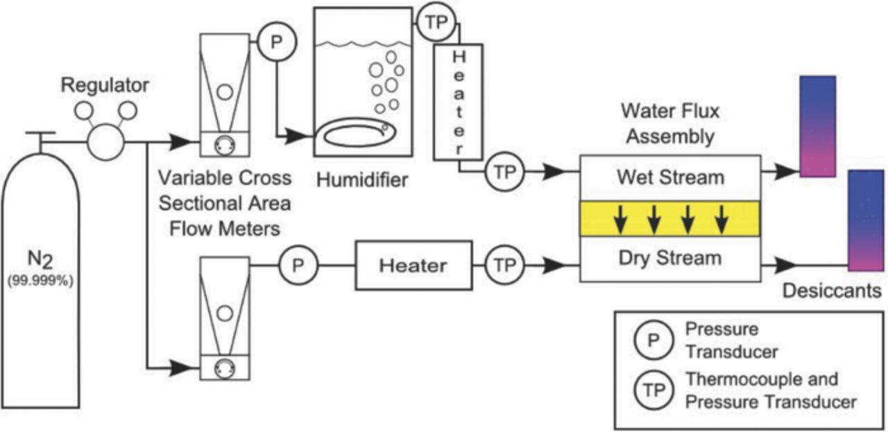
Figure 1. A schematic representation of the experimental setup. The water is able to transport across the membrane from the wet stream to the dry stream before being captured in the desiccants.
A SnowPure Excellion I-200 AEM was used for the experiments conducted for this study. This AEM has a polypropylene backbone. An ion exchange process was performed by following the process used by Vega et al. to convert the membrane from the chloride to hydroxide form.6 The membrane was soaked in 10−4 M potassium hydroxide (KOH) solution for 24 hours. Using higher concentrations KOH solution has shown significant degradation of the membrane within a few days.6 After soaking in KOH, the membrane was rinsed and soaked in deionized water to remove KOH from the membrane. This step was done twice over a 24 hour period. The fully hydrated membrane was then installed in the water flux experiment assembly.
The experiments performed for this work measure the mass of the water transported through the membrane along the length of a serpentine flow channel. Nitrogen (Airgas, Ultra High Purity) was used as an inert carrier gas to create a concentration gradient of water across the membrane. The nitrogen is split into two gas streams, labeled "Wet" and "Dry". The two streams are regulated to the same flow rate and heated to the operating temperature of the cell to minimize any effects arising from temperature gradients; however, such effects may be considered in future works. The dry stream goes directly into the cell whereas the wet stream is humidified to create a water concentration gradient across the membrane. This is completed with a bubble humidifier (Scribner), which adds deionized water to the gas stream based on the temperature of the water bath. The gas stream leaves the humidifier fully saturated at the water bath temperature. Based on the operating temperature of the assembly and the desired relative humidity, saturation tables for water are used to find the necessary partial pressure and bath temperature of the water.
The AEM was installed between two graphite plates with parallel serpentine flow channels. Only the membrane was used for the measurements. This removed any effects that could be seen from a gas diffusion layer or catalyst layer; isolating water transport in the AEM. The graphite plates were held together with two stainless steel end plates and a series of 8 bolts. These bolts were tightened to 5.65 N-m (50 in-lb) to ensure a proper seal. A cartridge heater was inserted into each of the endplates to maintain the operating temperature of the assembly. The heaters were controlled using temperature controllers and a K-type thermocouple (Omega) which was inserted into one of the endplates for feedback.
The two gas streams enter the cell with a water concentration gradient across the membrane. This causes water to diffuse across the membrane from the wet stream to the dry stream. This process occurs along the length of the flow channel. Once reaching the end of the cell, the gas streams exit the cell and travel through a desiccant (Drierite). The desiccant is capable of capturing most of the water, leaving nitrogen with a dew point of −70°C. Knowing the initial and final weight of the dry side desiccant tube, an average weight flux across the membrane can be computed.
All of the trials were conducted such that the membrane had time to equilibrate and the local hydration and water flux remained constant with time. The assembly was operated at 50 and 60°C and the flow rate of the gas entering the cell was varied between 25 and 700 sccm. To reduce any water permeation resulting from total pressure gradients across membrane, and therefore isolate diffusion, the flow rate was first set on the dry side of the membrane. The flow rate on the wet side of the membrane was then set to match the back pressure of the dry side. Less than 10% differences in flow rate between the wet and dry streams were recorded with this method. The humidifier was set such that the wet gas stream was entering the cell at 95% relative humidity. The experiment was first validated using DuPont Nafion 117 PEM before switching to the SnowPure Excellion I-200 AEM.
Theory
Water-membrane diffusion coefficient
To calculate the water-membrane diffusion coefficient, a numerical model was used to simulate the water flux experiment. This model entails a marching scheme along the length of the flow channel to solve for the water distribution in the gas stream and in the membrane.23 The initial water concentration going into the cell is known and is used as an initial condition. Performing a mass balance on smaller control volumes allows for distribution of water concentrations in the two gas streams and water content in the membrane to be solved along the length of the channel. The water content in the membrane is correlated to the water concentration in the gas stream based on absorption curves. Using Fick's law, the flux through the membrane in a given control volume can be calculated. The water concentration in the gas channel can then be updated for the next control volume until the end of the flow channel is reached. Using the experimental data with the numerical model, the diffusion coefficient in the model can be calculated to best match the water flux results. The diffusion coefficient was calculated as a second order polynomial function of water activity, which is iterated to find the coefficients to the polynomial such that agreement exists with the experimental data. This procedure was validated with Nafion 117 PEM and then applied to the Excellion I-200 AEM.23
Ionic conductivity model
With the water-membrane diffusion coefficient determined, a method is needed to relate the water-membrane diffusion coefficient to the ionic conductivity in the membrane. This can be accomplished using the dusty fluid model (DFM) and Ohm's law. Starting with the generalized Stefan-Maxwell diffusion equations, the DFM can be derived where, the membrane is treated as a separate species that interacts with the diffusing media but is fixed in space.24 The membrane, or "dust," particles are uniformly distributed and can represent the side chain groups of the membrane. Using the DFM, the flux of each species can be solved for. Assuming the side chains are uniformly distributed, a concentration gradient of mobile ions cannot exist according to the condition of electroneutrality. In this analysis, the interaction between the mobile ion species is assumed negligible. The total ionic conductivity of the membrane is then calculated as the summation of the individual conductivities in the system. The individual conductivities can then be calculated considering only two mobile species: water and the conducting ion (hydroxide, carbonate, or bicarbonate). Considering a closed electrochemical impedance spectroscopy cell, then it can be assumed that the two species have equal and opposite molar fluxes and are in pseudo-equilibrium.24,25 Manipulating the DFM and Ohm's law with these assumptions allows for the ionic conductivity to be solved in the membrane as seen in Eq. 1. Considering comparable assumptions, a similar equation can be derived starting with the Nernst-Planck equation.
![Equation ([1])](https://content.cld.iop.org/journals/1945-7111/160/9/F994/revision1/jes_160_9_F994eqn1.jpg)
Using Eq. 1, the ionic conductivity of the membrane can now be calculated based on several important variables. The first term is a constant which is comprised of Faraday's constant, F, valence of the ion, zi, the universal gas constant, R, and the temperature of the system, T. The diffusion coefficient in the pore is estimated by multiplying the infinite dilution diffusion coefficient in water, D0i, by a Bruggemann term which is a function of pore volume fraction, (ε − ε0)q. The denominator of that term contains a parameter, δi, which is the effective ratio of the infinite dilution diffusion coefficient to the ion-membrane diffusion coefficient. The final variables represent the concentration of ions in the pore of the membrane. The total concentration of ion i in the membrane is multiplied by a dissociation constant, αi, to yield the number of ions available for transport in the pore, Ci. Equilibrium constants are used in Eq. 2 to solve for concentrations of free ions, Ci, free fixed ions from the membrane, CM, and the number of ions attached to membrane, Ci · M. The dissociation constant for a species i is defined as the fraction of free (dissociated) ions available in the pore compared to the total number of that species in the membrane.
![Equation ([2])](https://content.cld.iop.org/journals/1945-7111/160/9/F994/revision1/jes_160_9_F994eqn2.jpg)
Ion-membrane diffusion coefficients
Using the experimental and numerical tools outlined above, a water-membrane diffusion coefficient is found. This diffusion coefficient needs to be corrected to be in an ion-membrane form to be useful in the ionic conductivity equation. In order to accomplish this, principles from kinetic theory are used which can convert from the water-membrane diffusion coefficient to an ion-membrane diffusion coefficient.
Kinetic theory, which was originally developed for low density monatomic gases where transport properties can be predicted based on collisions for non-interacting rigid spheres, is able to predict diffusion coefficients for most gas mixtures within a reasonable uncertainty. This is enabled by the relatively small interaction between molecules and serves as an approximation in this work. More rigorous derivations of the theory include interactions between molecules and more accurately predict transport properties for dense gases and liquids. For these conditions, the specific details of the nature of forces between both individual and groups of neighboring molecules are more significant and should be considered for the most accurate prediction. For a system in the membrane, the forces between molecules can be significant given that it is in liquid phase and contains ions. The ions in this system can, in the presence of water, form a solvation shell which reduces the charge effects from the ion. Considering this solvation shell, a hydrated ion can be assumed to transport through the membrane with similar inter-molecular forces to a single water molecule. These forces are captured in the water-membrane diffusion coefficient which was measured experimentally. Therefore, the water-membrane diffusion coefficient which was measured can be scaled using predictions from kinetic theory to arrive at a diffusion coefficient of the ion in the membrane.
Kinetic theory states that a diffusion coefficient between two species is going to be related to the speed of the particles and the mean free path.26 The average speed of the particles can be found based on a reduced mass of the two diffusing species, μij. If the particles are assumed to be rigid spheres, the average distance traveled between each collision for the particles is found using the collision radii of the particles, rij, as well as the total number density of the system, Nij. Knowing these properties, the diffusion coefficient between two species, i and j, can be found using Eq. 3.
![Equation ([3])](https://content.cld.iop.org/journals/1945-7111/160/9/F994/revision1/jes_160_9_F994eqn3.jpg)
The diffusion coefficient of water in the membrane is found experimentally. Starting with an identity relationship (Eq. 4a), the terms can be rearranged to solve for an ion-membrane diffusion coefficient by scaling the water-membrane diffusion coefficient (Eq. 4b).
![Equation ([4a])](https://content.cld.iop.org/journals/1945-7111/160/9/F994/revision1/jes_160_9_F994eqn4.jpg)
![Equation ([4b])](https://content.cld.iop.org/journals/1945-7111/160/9/F994/revision1/jes_160_9_F994eqn5.jpg)
Equation 3 can now be substituted into Eq. 4b to arrive at an expression for an ion-membrane diffusion coefficient as seen in Eq. 5. The diffusion coefficient which is calculated here is strictly a collision based diffusion coefficient and would not include other mechanisms for ion transport such as structural diffusion. This equation only depends on the water-membrane diffusion coefficient, reduced masses, collision radii and number densities of the diffusing species. These properties can all be calculated based on values found in Table I and reported in the literature.
![Equation ([5])](https://content.cld.iop.org/journals/1945-7111/160/9/F994/revision1/jes_160_9_F994eqn6.jpg)
Results and Discussion
The methodology for calculating the diffusion coefficient from the water flux experiment was validated by using the Nafion 117 PEM. This membrane was chosen for validation because of the volume of data and literature published on water-membrane diffusion coefficients and ionic conductivities. The water flux results from the experiment agreed with data from the published literature given the operating conditions. This validated both the experiment as well as the numerical water flux model.
The water flux across the Nafion 117 PEM increased with the operating temperature of the assembly. Raising the temperature typically increases the value of diffusion coefficients and given this trend, would cause greater water flux across the membrane. Also, maintaining the relative humidity of the incoming wet gas stream at 95% relative humidity yields more water per unit volume entering the assembly at 60°C than at 50°C. This would create a higher concentration gradient to drive diffusion. With Nafion 117, the water flux continued to increase with increasing flow rate. As the flow rate increases, the concentration on either side of the membrane is more likely to remain constant and therefore maintain a more uniform flux along the length of the channel.
When the experiment was repeated using SnowPure Excellion I-200 AEM, the water flux across the membrane was significantly lower than that of Nafion 117. This agrees with ionic conductivity data and would suggest that lower transport rates in the Excellion I-200 AEM. The decrease in water flux can also be explained by the increase in the thickness of the membrane. The Excellion I-200 AEM has a dry thickness of about 350 μm, while the Nafion 117 PEM has a dry thickness around 178 μm. The experimental data for Nafion 117 shows an increase in water flux with flow rate; however this trend was not true with the Excellion I-200. This is most likely attributed to a small water-membrane diffusion coefficient value. It can be seen in Figure 2 that there is a slight decrease in the water flux as flow rate increases for the Excellion I-200 AEM.
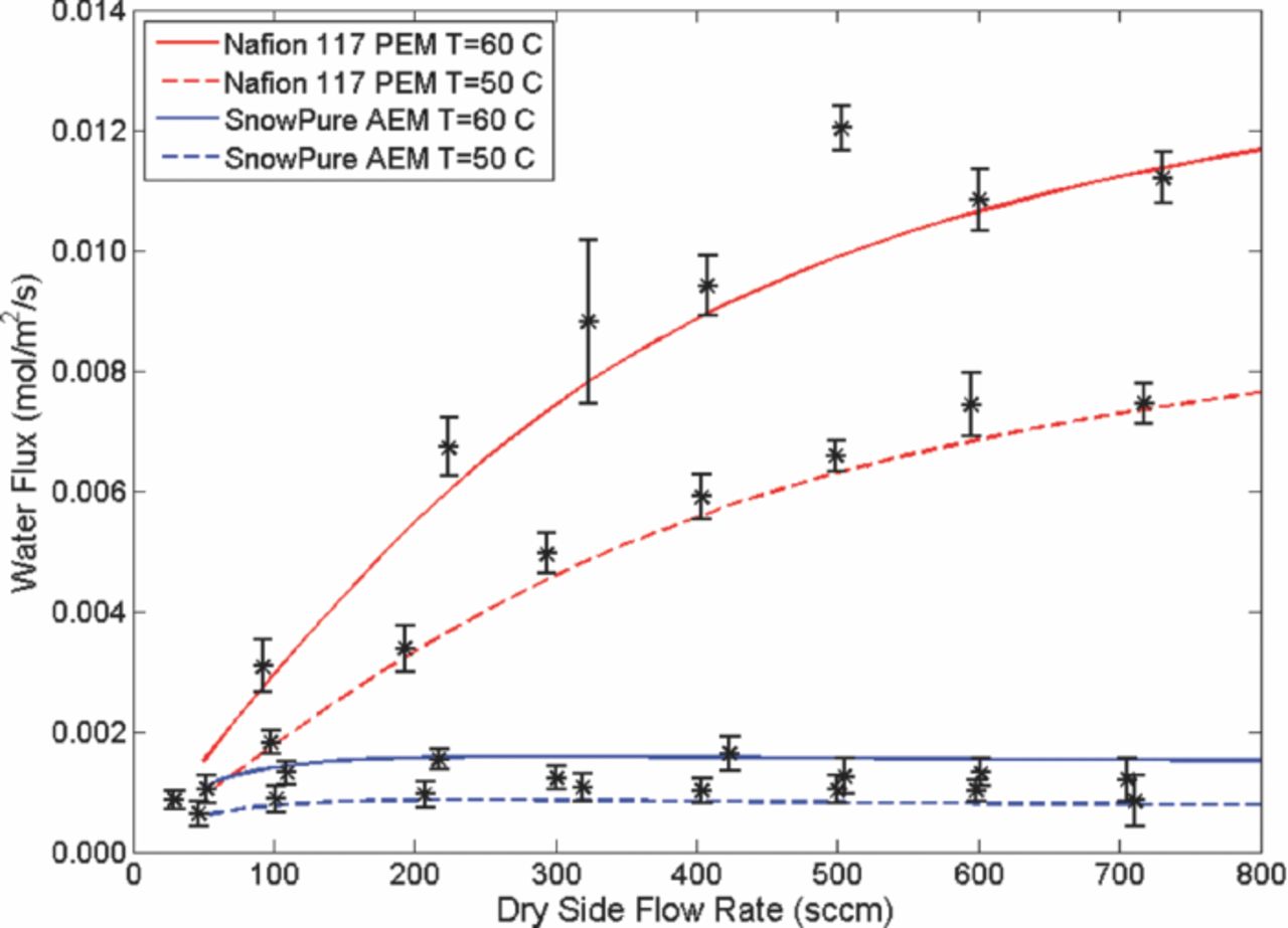
Figure 2. Water flux measurements for the two membranes. The experimental points are shown as symbols and the numerical model predictions are shown as lines.
With the water flux experiment and model validated using Nafion 117 PEM, a water-membrane diffusion coefficient could be found for Excellion I-200 AEM. This diffusion coefficient includes effects from the structure of the membrane, such as the tortuosity, as well as sorption effects.18,19,22,23 Currently the model does not include sorption effects, and agrees with reported diffusion coefficients for Nafion 117 PEM, suggesting that sorption effects have little effect in these experimental results.23 In an AEM system, the water flux through the membrane is significantly lower and therefore any sorption effects should be less significant than in a PEM system. The water-membrane diffusion coefficient for the Excellion I-200 AEM is about an order of magnitude less than that of Nafion 117 PEM. This is in agreement with the water flux measurements that show significantly less water diffusing through the AEM than the PEM.
To convert the water-membrane diffusion coefficient to an ionic form such as the hydroxide form, Eq. 5 can be used. Given that the species is transporting in the presence of water, hydrated values are used such that the primary solvation shell is considered. This accounts for several water molecules solvating an ion, increasing the mass and radius. The number of water molecules present in the solvation shell depends on the ion and ranges from 4 around hydroxide,27 to 6.9 around bicarbonate,28 and 8.7 to 9.1 around carbonate.28,29 Hydrated radius values were used based on Nightingale30 who correlated the Stokes radius to the hydrated ionic radius. The mass of the ion is simply a combination of the ion mass and the mass of the water molecules in the solvation shell. The hydroxide ion has the smallest hydrated radius and mass while the carbonate ion has the largest radius and mass. The number density of the carbonate species present in the membrane will be different than that of the bicarbonate and hydroxide ions. This is because of the −2 valence of the carbonate ion versus the −1 valence of the other species.
The diffusion coefficients for the SnowPure AEM are plotted in Figure 3 and all increase with increasing hydration in the membrane. The curves, especially for H2O, show a percolation limit at low hydrations where transport rates become inappreciable. The water-membrane diffusion coefficient has the lowest of the diffusion coefficients, when compared with the ion diffusion coefficient at higher hydrations, where the membrane would most likely be operated. With the pore volume fraction increasing with hydration, the ion-membrane diffusion coefficients increase as the species become diluted in the pore volume. The hydroxide ion has the highest diffusion coefficient in the membrane due to its relatively small size and mass. Hydroxide (and protons) are known to be subject to the additional transport mechanism known as Grotthuss transport, which can lead to their larger diffusion coefficients. Ions such as carbonate and bicarbonate are not subject to Grotthuss. The carbonate diffusion coefficient is the next largest despite having a larger mass and collision radius than the bicarbonate ion. This happens because the number density of the carbonate species is lower in order to maintain electroneutrality.
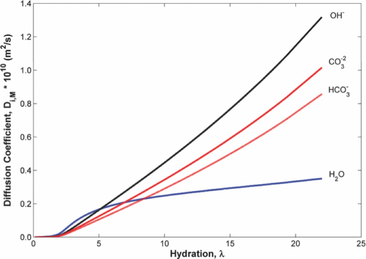
Figure 3. Ion-Membrane diffusion coefficients in SnowPure Excellion I-200 AEM. The hydroxide ion can transport across the membrane more easily than either the carbonate or bicarbonate ions.
With the diffusion coefficients for different ionic species, the ionic conductivity of the membrane can be calculated as a function of hydration. Using Eq. 1, the diffusion coefficients for the different species are substituted into the equation to yield the ionic conductivity. Results are shown in Fig. 4a for three membranes: Nafion 117 PEM, ETFE AEM, and SnowPure AEM. Experimental results provided by Vega et al. can validate the numerical predictions from the model.6 In order to best match the experimental value, the equilibrium constant used in Eq. 2 for the side groups and hydroxide is fitted within values reported in the literature.5,31 The trimethylammonium (TMA) hydroxide group is a strong base and the corresponding equilibrium constant (i.e., base constant) which was found is KTMA · OH = 0.37. Even with this equilibrium constant value, only a fraction of the hydroxide ions that are available for transport in the membrane are free and dissociated from the membrane. At fully hydrated conditions, roughly 32% of the hydroxide ions (counter ions) are dissociated from the side chain groups. To determine the dissociation, the fraction of free ions can be found using the concentrations of species calculated using Eq. 2. The dissociation is calculated by dividing the free concentration of hydroxide by the total concentration of hydroxide in the membrane. This approach was used by Thampan et al.25 for calculating the dissociation of protons in Nafion PEM. As the dissociation increases, more ions will be available for transport and the ionic conductivity will increase.

Figure 4. a) Ionic conductivities of several membranes as a function of hydration. Lines represent numerical predictions. Experimental points for the different membranes are shown as symbols: Nafion 117 PEM (□) Sone et al.33 and (△) Zawodzinski et al.,15 ETFE AEM (○) Varcoe,7 and SnowPure I-200 AEM, (*) Vega et al.6 b) For the SnowPure I-200 AEM, the hydroxide and combined carbonate and bicarbonate form is shown. In the carbonate and bicarbonate form, the ionic conductivity of the individual species as well as the combined ionic conductivity is shown. The ionic conductivities agree well with the reported values from Vega et al.6 shown as symbols.
With the approach outlined above, the water-membrane diffusion coefficient was experimentally measured for Nafion 117 PEM and SnowPure Excellion I-200 AEM. Knowing the water-membrane diffusion coefficient allows for the direct calculation of the δ parameter in Eq. 1. Unfortunately, an ETFE membrane was unavailable for testing and is discussed here as a comparison for the SnowPure Excellion I-200 AEM to another AEM. Previous studies for PEMs and AEMs have used δ as a fitting parameter because a water-membrane diffusion coefficient was unknown.24,25 In these works, δ was treated as a constant and was able to achieve reasonable agreement to experimental conductivity results. A least squares fit algorithm can be applied to experimental hydroxide conductivity results for ETFE AEM to arrive at values for δ and a percolation limit. A value of 1.65 can be found for δ and a percolation limit at λ = 3.16 was found for the AEM. These values are reasonable when compared to reported values by Grew and Chiu with δ = 1.90 and a percolation limit at λ = 2.50 for the ETFE AEM.24 It is difficult to compare the ionic conductivities of the ETFE AEM and SnowPure AEM since they have several differences including backbone polymer and ion exchange capacity. It can be noted that the ETFE AEM has a hydroxide ionic conductivity that is noticeably greater than the SnowPure AEM. However it is still roughly an order of magnitude less than the proton conductivity of the Nafion 117 PEM.
A further decrease in ionic conductivity was seen after ion exchange of the membrane into a carbonate and bicarbonate form. For the carbonate and bicarbonate results, Vega et al. treated the membrane in a solution of 0.5 M Na2CO3 and 0.5 M NaHCO3. Knowing this treatment, the ion concentrations in the external solution can be solved and used to predict ion concentrations in the membrane.5 This was done assuming an ideal membrane which has no preference to specific counter ions. Taking into account the ion concentration in the external solution and the valence of each ion, the membrane was found to be primarily in a carbonate ion form. Even though the membrane was assumed to have no preference to counter ion, the −2 valence of the carbonate ion makes it more preferable for the membrane.5 The mole fraction of the ions in the membrane was 60.75%, 38.62%, and 0.64% for carbonate, bicarbonate, and hydroxide respectively.
Knowing the ion concentrations in the membrane, the total ionic conductivity is assumed to be the addition of the ionic conductivity from each ion. With only a single experimental data point at fully hydrated conditions, it is difficult to separate the individual effects from the two mobile ions present in the membrane. In order to predict the dissociation of individual ions in the membrane, ions of the same valence are assumed to have equal equilibrium constants. Using this approach, the bicarbonate and hydroxide will use the same equilibrium constant and the carbonate equilibrium constant can be obtained using values from ions of the same valence in the literature.31 Using this approach, a value of  = 0.08 can be used for carbonate. This equilibrium constant is much lower than that of hydroxide in the membrane which means a smaller dissociation constant for carbonate ions. The individual contributions to the ionic conductivity are shown in Figure 4b. Carbonate contributes most given it has the highest concentration in the membrane and carries more charge with a −2 valence.
With the membrane being put in the carbonate/bicarbonate form, a decrease in performance is seen by both the model and the experimental results. This decrease in ionic conductivity agrees with the trend for the values calculated for the ion-membrane diffusion coefficients. If the ion has a lower diffusion coefficient, then it would be expected that the ionic conductivity would be lower for that ion as well. This model is able to successfully predict the performance for the membrane in the hydroxide form and match the experimental results. However, with the mixed ion form, the model over predicts the conductivity of the membrane. The model predicts total ionic conductivity of the membrane in the carbonate form to be 2.49 mS/cm where the experimental results show 2.25 mS/cm. This exceeds the experimental value by roughly 10%. This increase can be from several factors including over predicting ion-membrane diffusion coefficients or neglecting effects between the counter ions.
Using this model, the dissociation effects in the membrane can also be investigated. With Nafion PEM, there is almost complete dissociation between the fixed sulfonic acid groups and the protons.25 This helps contribute to the high ionic conductivity of Nafion PEM. Even with highly basic ionic groups, the ion dissociation in AEMs is much lower than in their acidic counterparts.32 For the SnowPure AEM with hydroxide counter ions at fully hydrated conditions, only 32% of the ions are free for transport in the pores. When the membrane is exchanged into the mixed carbonate/bicarbonate form, three ions are present and the total dissociation can be looked at for each ion as well as the total free charge in the pores. The hydroxide and bicarbonate are roughly 40% dissociated while the carbonate is only 20% dissociated at fully hydrated conditions. Another way to analyze these numbers is to consider the total charge of the free ions and compare that to the total charge available from the membrane. By considering the fraction of free charge, a direct comparison can be made between different scenarios with single or multiple counter ions. For this calculation, each free ion concentration is multiplied by its valence. The summation of the absolute values is then divided by the charge available in the membrane, the membrane concentration multiplied by its valence, to find the fraction of charge available for transport. For the hydroxide counter ion case, the fraction of charge available for transport in the membrane is the same as the dissociation of hydroxide in the pores. However, considering the total amount of charge free in the pores for the mixed ion form described above, only 25% of the charge is free in the pores. The mixed ion form has been shown experimentally and numerically to have a smaller ionic conductivity than the hydroxide form. This is explained by a decrease in charge available for transport, as well as lower ionic diffusion coefficients in the membrane.
Conclusions
In this study, a water flux experiment was built to measure total water flux through fuel cell membranes. In order to extract more information, a numerical model was developed to calculate the local hydration and water flux along the length of the flow channel. Using this model, the water-membrane diffusion coefficient was iterated until the total water flux in the numerical model matched the experimental results. This technique was validated using Nafion 117 PEM and then extended to solve for the water-membrane diffusion coefficient in SnowPure I-200 AEM. The water-membrane diffusion coefficient was then converted to an ion-membrane diffusion coefficient using principles from kinetic theory. This method scales the measured water-membrane diffusion coefficient by ratios of known parameters such as reduced mass, collision radius and number density. Finally, using a conductivity equation derived from the dusty fluid model, the ionic conductivity of the membrane is obtained using the calculated ion-membrane diffusion coefficients. The results have been validated to ionic conductivity results found in the literature for the ETFE AEM and the SnowPure I-200 AEM.
Acknowledgments
Financial support from the Army Research Office (award number W911NF-12-1-0148) is gratefully acknowledged. KNG gratefully acknowledges support from the U.S. Department of the Army and U.S. Army Materiel Command.