Relativistic magnetohydrodynamics winds from rotating neutron stars

Abstract

1 INTRODUCTION

Magnetically dominated winds from stars and accretion discs are central to the angular momentum evolution of these objects. Because they can efficiently extract rotational energy – transforming stored gravitational binding energy into asymptotic wind kinetic energy – magnetic outflows are ubiquitous in powering a wide variety of astrophysical systems. Schatzman (1962) first introduced the key idea that a magnetic field anchored in a rotating star with a wind can enforce plasma corotation out to radii large compared to the stellar radius, thus greatly increasing the angular momentum lost per unit mass.

Ideas of Schatzman (1962) were formalized in the steady non-relativistic flow model of Weber & Davis (1967), who assumed a pure monopole field geometry, and then by Mestel (1968a,b) who assumed a more realistic dipole magnetic field configuration. For strong dipole fields, a closed zone forms at low latitudes and the mass-loss is concentrated at high latitudes in regions where the field lines can be opened. If the extent and shape of the open field line region is known, then the physics of the magnetic wind is similar to that in the monopole geometry: the flow emerges along the open flux tubes and its character is determined by passing through the slow-magnetosonic (SM), Alfvén (AL) and fast-magnetosonic (FM) surfaces. If the thermal sound speed is small, the flow is driven primarily by magnetocentrifugal forces and the asymptotic outflow velocity is approximately v_A(R_A) ≈R_Aω, where R refers to the cylindrical radius, ω is the stellar angular velocity, and R_A is the AL radius. Because R_A is the point at which B²(R_A)/4π=ρv²_A(R_A), the outflow kinetic energy is roughly equal to the magnetic energy. This remains true in the asymptotic wind.

The theory of magnetic winds has been greatly extended and applied in its non-relativistic form to a wide variety of problems in stellar astrophysics. Gosling (1996) and Aschwanden, Poland & Rabin (2001) provide reasonably modern reviews in the solar context, where many of the recent developments in non-relativistic wind modelling have occurred. Multidimensional models have been motivated in part by the fact that toroidal magnetic fields can collimate the flow along the rotation axis via hoop stress into jets, a topic of much interest in the modelling of the bipolar outflows observed from protostars (e.g. Smith 1998).

The discovery of rotation-powered pulsars motivated the extension of these ideas to relativistic flows and relativistically strong magnetic fields (B²/4π≫ρc² at the source), in order to account for the observed spindown of pulsars. Michel (1969) and Goldreich & Julian (1970) made the first extensions of the model of Weber & Davis (1967) to relativistic outflows, recovering the same sequence of critical points in the flow. As reviewed in Section 2, these studies yielded estimates of the spindown torque of

1

The dipole moment of the star, μ, was assumed to be related to the monopole moment m appearing in the magnetohydrodynamics (MHD) theory via m=μ/R_L, a relation equivalent to assuming that the AL radius R_A was equal to the radius of the Light Cylinder R_L=c/ω. Since these monopole models only treated the flow in the rotational equator, the numerical coefficient k∼ 1 in equation (1) could not be determined accurately.

These simplified theoretical models revealed important differences between relativistic and non-relativistic winds. First, instead of reaching approximate energy equipartition between flow kinetic energy and magnetic energy, the asymptotic flow remains strongly magnetized. The asymptotic Lorentz factor is given by γ_∞≈σ^1/3₀, where ⁠, Φ is the magnetic flux, and is the mass-loss rate. Thus, γ_∞≪σ₀. For a highly relativistic outflow (σ₀≫ 1) the asymptotic magnetization σ_∞=σ₀/γ_∞≈σ^2/3₀≫ 1. A second important difference is that in relativistic magnetized flows the electric force cannot be neglected.1 Although it is absent by symmetry in the Michel and Goldreich & Julian models, the electric force almost exactly cancels the focusing hoop stress in multidimensional monopole models, thus undermining the usefulness of these flows for the understanding of relativistic collimated jets. This is a problem generic to all relativistic outflows (Lyubarsky & Eichler 2001) not focused by some external medium (e.g. a disc or external channel).

Much effort has gone into relaxing the simplifications of these early models, and in particular, on understanding what is required for an ideal MHD flow to have γ_∞→σ₀. Observations and models of pulsar wind nebulae suggest that at the termination shock of the outflows of young rotation-powered pulsars, the magnetic energy has been almost completely converted into flow kinetic energy (the ‘σ problem’) and the flow 4-velocity has reached γ≈σ₀ (the ‘γ problem’), in contradiction with the predictions of the 1D monopole treatments. If the magnetic surfaces retain an almost monopolar shape the acceleration of the flow is only logarithmic (Begelman & Li 1994). However, various asymptotic solutions (Begelman & Li 1994; Heyvaerts & Norman 2003 and references therein) and similarity solutions (Vlahakis & Königl 2003; Vlahakis 2004) of parts of the full axisymmetric flow problem suggest that if the poloidal magnetic field is sufficiently non-monopolar beyond the FM point, the largely radial current that supports the toroidal magnetic field, might cross field lines toward the equator, causing a transfer of electromagnetic energy to flow kinetic energy. However, both a numerical solution in axisymmetric non-relativistic MHD (Sakurai 1985) and a perturbative calculation of relativistically magnetized MHD flow from the exact force-free solution (Beskin, Kuznetsova & Rafikov 1998) yield a poloidal magnetic field which hews closely to the exact monopolar form. Thus, the monopole puzzle of asymptotic winds with magnetic energy that is never converted to flow kinetic energy persists, suggesting that ideal MHD expansion of the wind contradicts the observations.

The monopole geometry for the poloidal field has long been recognized as a singular case. A dipole magnetic field aligned with the stellar rotation axis presents the simplest realistic alternative field geometry. Because the open field, where outflow occurs, has a nozzle shape that expands faster than r² at distances comparable to the radius of the last closed field line (r_Y), there is a possibility of faster acceleration and larger conversion of magnetic energy into kinetic energy than occurs in the monopole geometry. However, complete solutions in axisymmetric steady flow have only been possible for the monopole; the change of topology between closed and open field lines required in the dipole case has so far escaped solution of the Grad–Shafranov equation that describes the magnetic structure in MHD flows with inertia and pressure included.

The location of the AL radius in the outflow, and its relation to the maximum equatorial radius of the last closed field line r_Y, where typically a Y-type neutral point occurs in the magnetic field, is a problem of equal significance. As outlined in Section 2, if r_Y < R_L, and if r_Y/R_L is an appropriate function of ω, one might be able to account for the observed fact that in rotation-powered pulsars T_∥∝ωⁿ, with n < 3. The strong inferred magnetization of pulsars has always suggested that the outflow structure should be treated as a problem in force-free relativistic MHD, with inertial and pressure forces completely neglected (Goldreich & Julian 1969). The force-free Grad–Shafranov equation for the case of an aligned dipole (Michel 1973; Scharlemann & Wagoner 1973) resisted solution until recently (Contopoulos, Kazanas & Fendt 1999; Gruzinov 2005 assumed strictly force-free conditions everywhere, whereas Goodwin et al. 2004 included pressure effects near the Y-point). Gruzinov found that the torque is indeed given by equation (1), with k= 1 ± 0.1, while Contopoulos et al. (1999) found k= 1.85. All of these authors assumedr_Y=R_L, as is physically plausible.

However, subsequent work by Timokhin (2005) has found that force-free MHD allows a family of solutions with r_Y of the last field line within R_L, contrary to naive expectations. He found that k≈ 0.47 (R_L/r_Y)², which, when r_Y=R_L, is close to the force-free monopole result of Michel (1969). Importantly, these solutions indicate that beyond a few Light Cylinder radii, the poloidal magnetic field assumes a monopolar form, which suggests that acceleration in the asymptotic wind never reaches equipartition energies (the σ problem). However, since inertial forces are important beyond the FM surface (r≈σ^1/3₀R_L) the force-free approximation breaks down (Beskin et al. 1998; Arons 2004) and no strong conclusions may be drawn.

The ambiguities of the steady force-free models, and the difficulty of solving the magnetospheric structure in MHD with inertia and pressure included, suggest that an evolutionary approach to the problem would be useful. A time-dependent solution can then be sought for specified boundary conditions at the stellar surface (such as pressure or injection velocity). The system can then relax to a self-consistent steady state (if one exists) and this approach allows one to find the last closed flux surface unambiguously, for specified injection conditions. Furthermore, such a treatment allows for the possibility of intrinsic time dependence (including either limit cycle or chaotic behaviour) of the magnetosphere. The time dependence of individual radio pulses from rotation-powered pulsars, showing systematic drifting through the pulse window for many objects near the pulsar death line, and chaotic rotation phase over wider regions of the diagram (Rankin 1986; Deshpandhe & Rankin 1999) have time-scales consistent with global magnetospheric variability causing changes in the polar current system underlying pulsar emission (Arons 1981; Wright 2001). Indeed, the torque noise exhibited by many pulsars (Cordes & Helfand 1980) may also owe its origin to instabilities of the magnetospheric current system (Arons 1981; Cheng 1987a,b).

In this paper, we carry out time-dependent relativistic MHD (RMHD) modelling of both highly magnetized Poynting-flux-dominated winds (σ₀≫ 1) in which R_A≈R_L, as well as magnetized neutron star winds in which R_A is significantly less than R_L(σ₀≪ 1).

Large σ₀ MHD models draw their motivation from studies of rotation-powered pulsars and of magnetars (soft gamma ray repeaters and anomalous X-ray pulsars). More broadly, analogous problems appear in Poynting-flux-dominated models of jets from black holes and neutron stars. Low-σ₀ (but still magnetized) neutron star winds are of interest primarily in understanding the physics of very young neutron stars. In the seconds after collapse and explosion, the neutron star is hot (surface temperatures of ∼2–5 MeV) and extended. This proto-neutron star cools and contracts on its Kelvin–Helmholtz time-scale (τ_KH∼ 10–100 s), radiating its gravitational binding energy (∼10⁵³ erg) in neutrinos of all species (Burrows & Lattimer 1986; Pons et al. 1999). The cooling epoch is accompanied by a thermal wind, driven by neutrino energy deposition (primarily ν_en→pe⁻ and ⁠), which emerges into the post-supernova-shock ejecta (e.g. Duncan, Shapiro & Wasserman 1986; Qian & Woosley 1996; Thompson, Burrows & Meyer 2001).

A second or two after birth, the thermal pressure at the edge of the proto-neutron star surface, where the exponential atmosphere joins the wind (r_ν), is of order ∼10²⁸ erg cm⁻³ and decreases sharply as the neutrino luminosity (L_ν) decreases on a time-scale τ_KH, as the star cools and deleptonizes. The thermal pressure at the stellar surface is set by L_ν. If the proto-neutron star has a surface magnetic field of strength B₀, then at some point during the cooling epoch the magnetic energy density will exceed the thermal pressure. For fixed B₀, the wind region becomes increasingly magnetically dominated as L_ν decreases. For larger B₀ the magnetic field dominates at earlier times. For magnetar-strength surface fields (B₀∼ 10¹⁴–10¹⁵ G) the magnetic field dominates the wind dynamics from just a few seconds after the supernova (Thompson 2003).

Magnetars are thought to be born with millisecond rotation periods (Duncan & Thompson 1992; Thompson & Duncan 1993), in which case the combination of rapid rotation and strong magnetic fields makes the proto-neutron star wind magnetocentrifugally driven. Because the rotational energy of a millisecond magnetar is very large (∼2 × 10⁵² erg) relative to the energy of the supernova explosion (∼10⁵¹ erg) and because the spindown time-scale (where r_NS is the neutron star radius) can be short for large r_A, these proto-magnetar winds have been considered as a mechanism for producing hyperenergetic supernovae (Thompson, Chang & Quataert 2004). Because the wind becomes increasingly magnetically dominated and the flow eventually becomes Poynting-flux-dominated as the neutrino luminosity abates, the outflow must become relativistic. For this reason, proto-magnetar winds have also been considered as a possible central engine for long-duration gamma ray bursts (GRBs) (Usov 1992; Thompson 1994; Wheeler et al. 2000; Thompson et al. 2004). They may also be the source of ultrahigh energy cosmic rays (Blasi, Epstein & Olinto 2000; Arons 2003). The time dependent RMHD models of neutron star winds calculated in this paper provide a significantly improved understanding of proto-magnetar winds, and their possible role in hyperenergetic supernovae and GRBs.

1.1 This paper

With these goals in mind, in Section 2 we first outline some order-of-magnitude estimates for the spindown of neutron stars in both the low- and high-σ₀ limits. In Sections 3 and 4, we describe the details of our numerical model. In Section 5, we present our numerical results for the 1D monopole (Section 5.1), the 2D monopole (Section 5.2) and the aligned dipole (Section 5.3). In each case, we present a set of models for both low- and high-σ₀ winds. Finally, in Section 6 we present a discussion of our results and speculate on their implications for the spindown of rotation-powered pulsars and very young, rapidly rotating magnetars.

2 PHYSICAL MODEL

As a guide to the numerical models, we describe here several simple order-of-magnitude estimates of the properties of both high- and low-σ₀ winds from neutron stars.

2.1 Poynting-flux-dominated spindown

Consider a star with a magnetic dipole moment μ. For simplicity, assume μ∥ω. Suppose there is an outflow of plasma along open field lines which connect to the star in a polar cap, with the magnetic flux of the open field lines being Φ_o. The expected poloidal magnetic structure is shown in Fig. 1. In the closed zone, plasma corotates, and the toroidal currents, composed of corotating charge density and pressure and inertial drifts across the magnetic field, cause the distortions from the ‘vacuum dipole’ field, which are of importance at radii comparable to r_Y. Assume the AL radius R_A is comparable to r_Y. The Poynting flux is S= (c/4π) E×B, whose radial component is, with the poloidal electric field E=−(ω×r) ×B_p, S_r=−(ωrsin θ/c)B_p. With B_p(r_A) ≈B_dipole(r_A) and B_φ(r_A sin θ) ≈−B_p(R_A), S_r(R_A) ∼ (ωR_A/4π) μ²/R⁶_A, where subscripts p and φ denote the poloidal and toroidal components, respectively. Then the EM spindown torque is approximately

2

the evaluation of the constant k in equation (1) to be equal to 2/3 is the exact result for the EM torque on the force-free monopole (Michel 1973), which has no closed zone or Y-point. Since the open magnetic flux is Φ_o≈ (μω/c) (R_L/r_Y), the torque can also be written as T_∥≈ (2/3) (Φ²_oω/c) (r_y/R_L)².

Figure 1

Open in new tabDownload slide

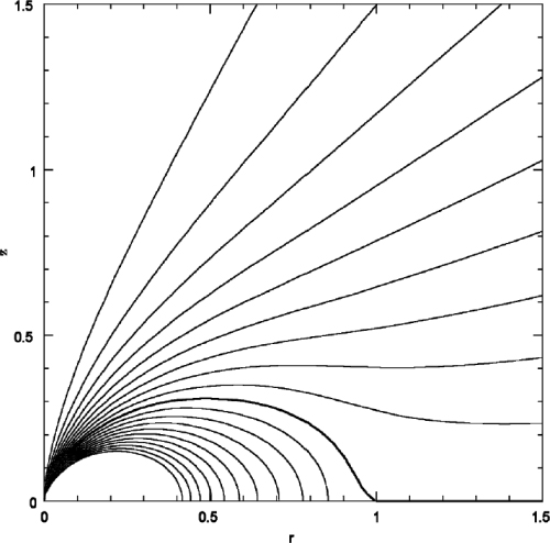
Force-free poloidal magnetic field lines from a magnetized star with dipole axis aligned with the rotation axis. The distances are scaled in units of the radius of the Light Cylinder, R_LC. From Gruzinov (2005).

If mass loading (inertial forces) and pressure are negligible, the long-standing expectation has been r_Y=R_A=R_L=c/ω (Goldreich & Julian 1969), and MHD spindown torques then should have braking index ⁠, if μ and the stellar moment of inertia are constant. Two numerical solutions for steady flow from the force-free aligned dipole rotator have found k= 1.85 (Contopoulos et al. 1999) and, at higher resolution, k= 1 ± 0.1 (Gruzinov 2005), rather than 2/3. The equality r_Y=R_L=R_A was assumed in both of these calculations.

A long-standing empirical puzzle has been that in the four observations of braking indices not requiring major corrections for glitches in the timing, the braking index lies between 2.5 and 2.9 (Lyne, Pritchard & Graham-Smith 1993; Kaspi et al. 1994; Deeter, Nagase & Boynton 1999; Camilo et al. 2000; Livingstone et al. 2005). This reduction of the braking index for fixed μ and ω, in comparison to our simple estimate, is tantamount to r_Y < R_L. That is, the closed zone ends within the Light Cylinder, 2and, as the star ages (ω decreases), r_Y/R_A also decreases – the magnetosphere becomes more open with decreasing spindown power. One way to state this is to simply assert that R_A=r_Y < R_L and that r_Y/R_L∝ω^α (e.g. r_Y/R_L= (ωr_NS/c)^α; Arons 1983). This implies a change in the polar cap size from r_NS(r_NS/R_L)^1/2 to the larger value (larger Φ_o) of r_NS(r_NS/R_L)^(1−α)/2. Using this expression, the braking index data require 1/6 ≥α≥ 1/30, with the largest value for the Crab pulsar and the smallest for the 407-ms pulsar J1119−6157.

Assuming α > 0 is equivalent to the last closed field line of the dipole having equatorial radius r_Y less than R_A≈R_L. According to our estimate (2), the electromagnetic torque depends on the field strength at R_A, which is noticeably larger than that estimated by using a pure dipole filed, since the poloidal field becomes progressively more monopolar for r > r_Y. Thus, one obtains a better estimate of the torque by using a simplified model of the poloidal magnetic field which has the correct asymptotic form shown by the force-free aligned rotator models – dipolar at r≪r_Y and monopolar at r≫r_Y. Our RMHD results have the same asymptotic behaviour. Thus, with B_p= (μ/r³) +κ(μ/r_Yr²), the same order-of-magnitude argument that led to (2) yields

3

4

Assuming the magnetic moment and the stellar moment of inertia (and i=∠ (ω, μ) are constant, and that R_A=R_L, a correspondence assumed in most force-free models and also found in the RMHD results we report below, one readily finds

5

Thus, a braking index less than 3 requires R_A/r_Y to depend on ω (more generally, to depend on time). If the time dependence of r_Y/R_A enters solely through dependence on ω, n < 3 requires R_A/r_Y=R_L/r_Y to increase as the star spins down – the magnetosphere becomes more open with time, and the magnetic field at the Light Cylinder to remain larger, than is expected in the traditional model. Such behaviour requires transformation of closed field lines to open, which can occur if magnetic dissipation at and near the Y-point allows reconnection to enable this transformation.

Our RMHD numerical results presented in Section 5.3 show that although R_A→R_L as soon as σ₀ exceeds unity, r_Y/R_L remains substantially less than unity for σ₀ as large as ∼20. We also find that, for σ₀ of order a few, the ratio r_Y/R_L decreases as ω decreases – the braking index in our models is less than 3. This suggests that seemingly small inertial and pressure forces can have a large effect on the magnetospheric structure and, in turn, the magnitude of the spindown torque and the braking index.

The work of Mestel & Spruit (1987) may provide an explanation for our numerical results. In their isothermal, non-relativistic analysis of the magnetohydrostatic equilibrium of the closed zone, they find that R_Y/r_NS depends crucially on the ratios V²_e/2c²_T and ω²r²_Y/V²_e, where V_e is the escape velocity from the stellar surface (see their Section 2 and equation 8). For r_Y a few times r_NS one finds an approximate implicit equation for r_Y:

6

One sees that for fixed isothermal sound speed c_T, if (ωr_Y/V_e) is greater than unity, then it becomes exponentially harder to increase R_Y/r_NS by increasing B²₀/ρ_NS.

However, since electromagnetic stresses alone can lead to Y-point formation, as is clear from the solutions of the force-free Grad–Shafranov equation, one should treat these estimates of R_Y as a function of plasma stress alone with caution, when applied to the magnetically dominated regime. Simplified models along the lines pioneered by Goodwin et al. (2004) may be helpful, but at present, the best results are the simulations themselves (Section 5.3). We defer a relativistic generalization of Mestel & Spruit (1987) with a polytropic (p∝ρ^Γ) equation of state (more appropriate to our simulations) to a future paper.

2.2 Spindown by magnetized mass-loaded winds

Stresses due to mass loading become significant in the thermally driven winds of newly born neutron stars. These stars may have strongly mass-loaded winds which have r_A large in comparison to r_NS, but significantly smaller than R_L (Thompson et al. 2004). Conditions for such winds in the presence of thermally driven mass-loss generally obtain when the isothermal sound speed c_T is smaller than, or of order, the AL speed, v_A.3

The torque on the star by the magnetized wind is easily estimated for a strictly monopolar field geometry (B_p∝r⁻²). At r_A we expect the poloidal magnetic energy density to be of order the radial kinetic energy density, B²_p/8π≃ρv²_r/2, and if c_T is much smaller than v_A, then we further expect that v_r(r_A) should be of order v_φ(r_A). A simple estimate for v_φ(r_A), which again requires that v_A≫c_T, is v_φ∼r_Aω. We combine the above ingredients to obtain an expression for the AL point:

7

where we have assumed that and B₀ is the magnetic field strength at the stellar surface. The time evolution of the spin period of the star is then governed by the equation

8

The rotational energy-loss rate is ⁠. In this limit (v_A≫c_T) the sonic point is approximately

9

where we have scaled the spin period P to 1 ms and r_Sch is the Schwarzschild radius. In the c_T≪v_A limit, the radial velocity reaches its asymptotic value of v_∞≈ (3/2)v_A at the FM point (e.g. Belcher & MacGregor 1976).

In the regime we are interested in this paper we always have a supersonic outflows at the AL surface. In this case, according to the standard parameterization of MHD winds (Sakurai 1985; Daigne & Drenkhahn 2002), all solution should be considered centrifugally or marginally centrifugally driven.

A similar set of estimates for a dipole magnetic field is considerably more complicated, particularly since, as in Section 2.1, the position of the Y-point is not known a priori. In addition, since the areal function along open flux tubes adjacent to the closed zone deviates significantly from radial, a full numerical solution is required to address spindown in this context (Section 5.3). However, as a rough guide in understanding the expected differences between monopole and dipole spindown it is sufficient to imagine the scalings for the dipole as essentially those for the monopole, but with the surface magnetic field strength normalized to just the open magnetic flux.

2.3 Parametrization

These estimates and those of Section 2.1 reveal the parameters which specify the physical regimes of relevance to our models of rotating magnetospheres. Mass-loss is thermally and centrifugally driven in these models, depending upon the ratio of pressure and centrifugal forces to the gravitational force, parametrized at the injection surface (r_in) by (c²_T/V²_e)$r=rin$ and by (Ωr_in/V_e)²$r=rin$. All of the models considered in this paper have the first of these parameters between 0.01 and 0.1, while the second is between 0.05 and 0.3. The values adopted can be derived from the parameter shown in Tables 1 (Section 4.1). For all of the 2D monopole and dipole models, magnetic pressure dominates gas pressure, as expressed by B²/4πc²_s > 1. This is true for most of the 1D monopole models also. Again, these parameters are listed in Table 1. In all cases, the thermal energy density is smaller than the rest-mass density (p < ρc²). Thus, pressure forces do not lead to relativistic motion. The values of the ratios between the characteristic speeds at the base of the wind, for all our simulations, are provided in Appendix A.

The distinction between pressure-driven and centrifugally driven wind, can be also done based on the conditions at the AL surface. In Daigne & Drenkhahn (2002) (following Sakurai (1985)) the distinction is based on the value of the ratio Γp/ρ(Ωr)² at the AL surfaces (Γ is the adiabatic coefficient). In all our cases this ratio is less than 0.1.

The most significant parameter is Michel's magnetization parameter, σ₀, defined just after expression (1). When the magnetic energy density exceeds the rest-mass density (σ₀ > 1), magnetic pressure can accelerate the flow to relativistic velocities. This parameter is listed for all the models, as our major goal is to span the regimes from highly mass loaded, pressure-driven, non-relativistic outflow (σ₀≪ 1) to lightly mass loaded, magnetically driven relativistic outflow (σ₀≫ 1) in both monopole and dipole geometry. The values of σ₀ for the various models are given in the tables in Sections 5.1–5.3.

We do not consider outflows driven by relativistically high temperature (p > ρc²), a regime more relevant to fireball models of GRBs.

3 MATHEMATICAL FORMULATION

The laws of mass and momentum–energy conservation, together with Maxwell equations in general relativity, are (Landau & Lifshitz 1971; Weinberg 1972; Misner, Thorne & Wheeler 1973; Anile 1989)

10

11

12

13

where ρ is the proper rest-mass density, u^ν and J^ν are the 4-velocity and the 4-current density, and F^μν is the Faraday tensor of the electromagnetic field. The momentum–energy tensor is given by

14

where g^μν is the metric, p is the gas pressure, and we have chosen a system of units in which c= 1. In the case of Γ-law equation of state for a perfect gas the specific enthalpy is h= 1 +Γ/(Γ− 1)p/ρ. In order to close the system, the current density J^ν must be specified in terms of the other known quantities, through an additional equation, Ohm's law. In the MHD approximation, Ohm's law becomes the condition that the net electric field in the fluid frame must vanish, which in covariant form reads

15

With this approximation, equations (10)–(13) can be rewritten in term of proper density, pressure, 4-velocity and magnetic field, reducing to a system of eight equations for eight variables, plus the solenoidal condition on the magnetic field, ∇·B= 0.

Although we consider winds from neutron stars with centrifugal forces large enough to affect the mass-loss, we only consider rotation rates slow enough to allow us to neglect rotational modifications of the metric. Therefore, we employ the Schwarzschild instead of the Kerr metric. The use of a diagonal metric allows one to simplify the equations and to implement them easily in any code for special relativistic MHD, as shown by Koide, Shibata & Kudoh (1999).

In Boyer–Lindquist coordinates (t, r, θ, φ) the diagonal elements of the metric are

16

where M is the mass of the central object (1.44 M_⊙).

In axisymmetry and steady state, equations (10)–(13) admit six integrals of motion along stream lines (flux tubes) (Camenzind 1986a, b, 1987; Daigne & Drenkhahn 2002):

17

18

19

20

21

22

where subscript p and φ indicate poloidal and azimuthal components, respectively, γ is the Lorentz factor, A is the area of the flux tube (A=r² in the case of radial outflow), and R=r sin θ the cylindrical radius. Again note that we have chosen units in which c= 1.

If the value of the six integrals is known on a stream line, then equations (17)–(22) can be solved for the value of primitive quantities like density, velocity and pressure. In general, quantities like and Φ are assumed to be known and given by the physical conditions at the surface of the central object, while the values of the remaining integrals are derived by requiring the solution to pass smoothly the SM, AL and FM points. In 2D, one also requires an additional equation for the area of the flux tube, and this is provided by requiring equilibrium across streamlines.

4 NUMERICAL METHOD

Equations (10)–(13) are solved using the shock-capturing code for relativistic MHD developed by Del Zanna, Bucciantini & Londrillo (2003). The code has been modified to solve the equations in the Schwarzschild metric following the recipes by Koide et al. (1999). The scheme is particularly simple and efficient, since solvers based on characteristic waves are avoided in favour of central-type component-wise techniques (Harten–Lax–van Leer solver based only on the FM speed). In the axisymmetric 2D approximation the equation for the evolution of B_φ can be written in conservative form and only one component of the vector potential, A_φ, is used in the evolution of the poloidal magnetic field. Moreover, we replace the energy conservation equation with the constant entropy condition, ⁠. Of course, this condition cannot be satisfied during the evolution when shocks form in the flow. However, if the wind evolves toward steady state, shocks propagate outside the computational domain, and the condition can be satisfied. There are various numerical reasons for our choice of S= constant. Most importantly, enforcing constant entropy significantly enhances code stability. For example, it is known that in strongly magnetized flows or in the supersonic regime, in deriving the thermal pressure from the conserved quantities, small errors can lead to unphysical states. In non-relativistic MHD, these unphysical states correspond to solutions with negative pressure. A common fix is to set a minimum pressure ‘floor’ that allows the computation to proceed. However, in RMHD it is possible that no state can be found (not even one with negative pressure) and the computation stops. This usually happens for high Lorentz factor γ∼ 10–100, depending on the grid-flow geometry, or in the case of high magnetization, B²/(ρh) ≳ 100. When the magnetization at the Light Cylinder is high, close to the central object it will be above this stability threshold, which prevents us from using the full equation of energy. The use of a constant entropy condition also greatly simplifies the derivation of primitive variables from the conserved quantities, thus increasing the efficiency of the code.

Lastly, by specifying the value of the entropy we remove entropy waves from the system. Entropy waves travel at the advection speed (and are dissipated in an advection time). If the sound speed is much smaller than c, the advection speed v_r, close to the surface of the central object, is much smaller than the speed of light and the advection time can be extremely long. By removing entropy waves, perturbations are dissipated at the SM speed, which in our regime is of the order of 0.1 c.

Simulations were performed on a logarithmic spherical grid with 200 points per decade in the radial direction, and a uniform resolution on the θ direction with 100 grid points between the pole and the equator (Courant–Friedrichs–Lewy factor equal to 0.4). Higher resolutions were used in a few cases, to test convergence and accuracy. In order to model the heating and cooling processes using an ideal gas equation of state we adopt an adiabatic coefficient Γ= 1.1 (almost isothermal wind), which is reasonably representative of the wind solution by, e.g. Qian & Woosley (1996). It can be shown that in order to have a transonic outflow the thermal pressure cannot be too high (above a critical value depending on Γ the sonic point moves inside the surface of the star) nor too low (the Bernoulli integral must be positive), as shown by Koide et al. (1999) in the hydrodynamical case. The available parameter space increases for smaller Γ. The value we choose allows us to investigate easily cases with p/ρ∼ 0.05, especially in the dipole case where the strong flux divergence at the base is more important.

4.1 Initial and boundary conditions, and model parameters

Simulations in both 1D and 2D were initialized by using a hydrodynamical 1D radial solution obtained on a much finer grid (the relativistic extension of the Parker solution (Parker 1958), and projecting it on the initial magnetic field lines. In the monopole cases, initial poloidal magnetic field lines are assumed to be strictly radial while for the dipole cases we adopt the solution for the vacuum dipole in the Schwarzschild metric (i.e. Muslimov & Tsygan 1992; Wasserman & Shapiro 1983). Density and pressure were interpolated from the hydrodynamical solution, v_r was derived by projecting the radial velocity on the magnetic field lines, and we set v_θ= 0. We also impose corotation in the inner region v_φ= min (ΩR/α, 0.6c), in order to avoid sharp temporal transients in the vicinity of the inner boundary.

Standard reflection conditions are imposed on the axis, and symmetric conditions are imposed on the equator. At the outer radial boundary, we apply standard zeroth order extrapolation for all the variables. Initial conditions are chosen in order to guarantee that during the evolution the FM surface is inside the computational domain so that no information is propagated back from the outer boundary.

Unfortunately, as we will discuss in the following section, in the 2D case such a constraint can not be satisfied close to the axis, unless one uses an excessively large computational domain. In a few cases, using larger grids that allow the FM surface to be inside the computational domain, we find that the results do not change appreciably except along the axis itself. That is, the global solution at all but the highest latitudes is not significantly affected by the fact that the FM surface is outside the computational domain very near the polar axis.

Particular care has to be taken for the inner boundary conditions. As pointed out in Section 1, we are here interested in the transition from mass loaded (σ₀≪ 1) to high-σ₀ winds, and our injection conditions are tuned to be as close as possible to the neutrino-driven proto-neutron star case. We chose the inner radius r_in to be located at 11 km (1.1 radii of the neutron star r_NS), which corresponds to the outer edge of the exponential atmosphere for a thermally driven wind (e.g. Thompson et al. 2001). The modelling of such a steep atmosphere requires very high resolution in order to avoid numerical diffusion, and the problem becomes prohibitive in terms of computational time in 2D. At the inner boundary the flow speed is smaller than the SM speed, implying that all wave modes can have incoming and outgoing characteristics. This constrains the number of physical quantities that can be specified. Density and pressure at the inner radius are set to be p/ρ∼ 0.04, thus fixing the entropy for the overall wind. The radial velocity is derived using linear extrapolation. We also fixed the value of Ω/α(r_in), typically at Ωr_in/α(r_in) = 0.2, corresponding to a millisecond period (in the neutron star proper frame, see also equation 24), which implies R_L= 6.8 r_NS.

The frozen-in condition (15) requires that the electric field in the comoving frame at the inner radius vanishes: v_p∥B_p→E_φ= 0 and E_p=ΩR_inB_p/α(r_in). The condition on E_φ implies that the radial component of the magnetic field remains constant. We chose for B_r(r_in) different values to investigate both cases with low magnetizations and high magnetization. B_θ and B_φ where extrapolated using zeroth order reconstruction (we found that linear interpolation can lead to spurious oscillations). The value of the tangential velocities were derived using the remaining constraint of the frozen-in condition: v_θ=v_rB_θ/B_r and v_φ=ΩR_in/α(r_in) −v_rB_φ/B_r. Given that the three components of the velocity are derived independently, there is no guarantee that v² < 1; so care has to be taken to avoid sharp transients and spurious oscillations in the tangential magnetic field near the inner boundary.

In Table 1 the parameters of our various models are given. Equations (17)–(22) show that the problem can be parametrized in terms of the ratio (assuming B_φ scales as B_r) and not on the specific value of density and magnetic field; more generally the parameter governing the properties of the system is (Michel 1969). The bulk of our simulations have been done using a fixed value for Ω, in order to allow a more straightforward comparison among the various results; however in a few cases (B1 of the 2D monopole, and B1, B2 of the 2D dipole) we use a different rotation rate to check whether the energy and angular momentum loss rates indeed only scale with σ₀. We note that it is computationally more efficient to increase the magnetic flux than to drop the mass flux in order to achieve higher σ₀. Only in the 1D case, where resolution is not a constraint, are we able to investigate the behaviour of the system for different values of ⁠.

5 RESULTS

5.1 The 1D monopole

As a starting point for our investigation, we consider the simple case of a relativistic monopolar wind in 1D. This is the relativistic extension of the classic Weber–Davis solution for a magnetized wind (Weber & Davis 1967), and represents a simplified model for the flow in the equatorial plane. The 1D model can also be used both to verify the accuracy of the code and as a guide in understanding the 2D simulations (Section 5.2 and 5.3). Here we assume v_θ=B_θ= 0. The solenoidal condition on the poloidal magnetic field reduces to B_r∝r⁻².

We calculate a number of wind solutions for different values of the flux Φ and the entropy ⁠. The results are summarized in Table 2. Case A0 is a reference case for an almost unmagnetized wind, and it will be used for comparison with the weakly magnetized regime (A–D). As stated above, the solution can be parametrized in terms of ⁠. We have verified that the mass-loss rate depends strongly on the value of the sound speed at r_in, and drops rapidly as the pressure approaches the critical value for ⁠, which also depends on the magnetic field strength. In contrast, over the range of parameters studied, has a relatively minor dependence on the value of the magnetic field at fixed ⁠: increasing B_r(r_in)² by three orders of magnitude corresponds to an increase in by just a factor of ∼1.7 (compare models A0 and F in Table 2). The reason for this is that in all cases listed in Table 2 the AL point is larger than the SM point. Thus, the magnetocentrifugal effect of increasing the density scale height in the region interior to the SM point, where the mass-loss rate is set, is already maximized. For all the cases investigated, the value of Γp/ρ(Ωr)² at the AL point is always less than 0.1 (in Case A it is ≃0.1 while in case E it is ≃0.02). All the solution can thus be considered centrifugally driven. We expect and find a sharp drop in as we go to yet smaller magnetization. For example, in the purely hydrodynamical case without magnetic fields, ⁠, six times lower than for Case F.

Table 2

Results of the 1D models.

Model .	σ0 .	.	.	.	γ(100rNS) .	rA/RL .
A0	0.013	101	10.6	99.0	1.12	0.30
A	0.084	142	4.17	18.0	1.20	0.46
B	0.164	74	3.34	9.98	1.22	0.56
C	0.307	39	2.71	6.06	1.32	0.65
D	0.634	19	2.18	3.75	1.42	0.75
E	2.81	4.25	1.52	1.86	1.87	0.89
F	6.85	175	1.31	1.49	2.30	0.93
G	18.4	130	1.17	1.24	2.94	0.96
H	61.4	155	1.08	1.10	4.00	0.98
I	127	188	1.06	1.06	4.84	0.99

Model .	σ0 .	.	.	.	γ(100rNS) .	rA/RL .
A0	0.013	101	10.6	99.0	1.12	0.30
A	0.084	142	4.17	18.0	1.20	0.46
B	0.164	74	3.34	9.98	1.22	0.56
C	0.307	39	2.71	6.06	1.32	0.65
D	0.634	19	2.18	3.75	1.42	0.75
E	2.81	4.25	1.52	1.86	1.87	0.89
F	6.85	175	1.31	1.49	2.30	0.93
G	18.4	130	1.17	1.24	2.94	0.96
H	61.4	155	1.08	1.10	4.00	0.98
I	127	188	1.06	1.06	4.84	0.99

and ⁠. Values of are given in code units, see equations (23)–(27) for conversion to physical units. In all cases Ω= 0.143.

Open in new tab

Table 2

Results of the 1D models.

Model .	σ0 .	.	.	.	γ(100rNS) .	rA/RL .
A0	0.013	101	10.6	99.0	1.12	0.30
A	0.084	142	4.17	18.0	1.20	0.46
B	0.164	74	3.34	9.98	1.22	0.56
C	0.307	39	2.71	6.06	1.32	0.65
D	0.634	19	2.18	3.75	1.42	0.75
E	2.81	4.25	1.52	1.86	1.87	0.89
F	6.85	175	1.31	1.49	2.30	0.93
G	18.4	130	1.17	1.24	2.94	0.96
H	61.4	155	1.08	1.10	4.00	0.98
I	127	188	1.06	1.06	4.84	0.99

Model .	σ0 .	.	.	.	γ(100rNS) .	rA/RL .
A0	0.013	101	10.6	99.0	1.12	0.30
A	0.084	142	4.17	18.0	1.20	0.46
B	0.164	74	3.34	9.98	1.22	0.56
C	0.307	39	2.71	6.06	1.32	0.65
D	0.634	19	2.18	3.75	1.42	0.75
E	2.81	4.25	1.52	1.86	1.87	0.89
F	6.85	175	1.31	1.49	2.30	0.93
G	18.4	130	1.17	1.24	2.94	0.96
H	61.4	155	1.08	1.10	4.00	0.98
I	127	188	1.06	1.06	4.84	0.99

and ⁠. Values of are given in code units, see equations (23)–(27) for conversion to physical units. In all cases Ω= 0.143.

Open in new tab

Note that the value of γ reported in Table 2 is at a fixed position, r= 100r_NS, which is generally outside the FM point (see Fig. 2). Case I is an exception. For reference, the Lorentz factor at ∼300 r_NS is 7.8 for this model.

Figure 2

Open in new tabDownload slide

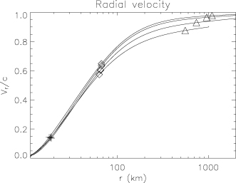
Radial velocity, and position of the SM (plus), AL (diamond) and FM (triangle) points, in the 1D monopole case. From bottom to top lines refer to Cases F, G, H and I.

All values in Table 2 are given in code units. The following relations can be used to scale to physical units, in terms of the value of density and magnetic field at the injection radius r_in. The mass-loss rate is

23

the rotation period is

24

the surface magnetic field strength is

25

the total energy-loss rate is

26

the angular momentum loss rate is

27

where and ⁠.

In Fig. 2, we plot the velocity profiles for Cases F, G, H and I, together with the location of the SM, AL and FM points. Note that the position of the SM point does not change significantly and is given roughly by equation (9). In Fig. 3, the angular momentum loss rate and energy loss rate are plotted as a function of σ₀. The convergence to the force free solution is evident (see also Table 2). An alternative way to parametrize how close the solution is to the force free limit is by considering r_A/R_L (Daigne & Drenkhahn 2002), as shown in Table 2. In the mass loaded cases (σ₀ < 1; models A–D) we find that in accord with the expectations from Section 2.2. We find that all the points (we excluded case A0 because we are interested in case where r_A > r_SM, typical of the transition from mass loaded to force free) can be approximated by a relation of the form ⁠, where C_o should correspond to the force free limit ⁠. A fit to our results gives C_o= 0.98 and C₁= 0.93. A similar expression can be written for the energy losses. At low σ₀ the total energy loss rate scales as the mass loss rate, as expected, ⁠. For large σ₀, the solution converges to the force free limit, (see Fig. 3). We find that the transition between the two limits can be fit with ⁠, where C_o= 0.98 and C₁= 2.16. We also consider the reduced energy loss rate (the difference between the total energy and the rest mass energy), and find that this too can be approximated with a power law: ⁠, with C_o= 0.98 and C₁= 0.965. We stress that these power law relations have been determined by fitting the results of our simulations. As such, there is no guarantee that these trends can be extended outside the range we investigated, but they do correspond well to the estimates given in Section 2.

Figure 3

Open in new tabDownload slide

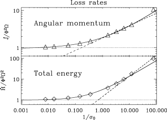
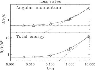
Loss rates for the 1D monopole calculations in non-dimensional units (Table 2). Upper panel: angular momentum loss rate. Lower panel: total energy-loss rate. Dashed curves represent the theoretical expectation for the losses in the mass loaded cases and ⁠. Continuous curves represent the best power-low fit given in the text. Dotted lines are the force-free solution.

Our simulations focus on the region close to the neutron star and so the problem of the acceleration of the outflow at large distances cannot be properly addressed. However, as shown, for example, by Daigne & Drenkhahn (2002) the efficiency of conversion from magnetic to kinetic energy in the strict monopole limit is very low. Faster than radial divergence in the flux tubes is required after the FM point to increase the acceleration significantly (Section 2.1). Within our computational domain in Case I we find that the ratio of particle kinetic energy flux to electromagnetic energy flux scales approximately as r^1/3 and shows a tendency towards saturation. At a radius of 300r_NS in Case I, the ratio is still less than 5 per cent.

5.2 The 2D monopole

The 1D monopole discussed above does not take into account deformations of the poloidal field lines by the moving plasma. As a consequence, the conversion of magnetic energy into kinetic energy of the accelerated wind is inefficient. To understand if and how deviations from a strict monopole may affect the dynamics of the outflow it is necessary to perform 2D simulations. We focus only on the region close to the star, within 100–200r_NS, and we consider both mass-loaded (σ₀ < 1) and Poynting-flux-dominated (σ₀ > 1) regimes (see Tables 1 and 3). In contrast to the cases considered by Bogovalov (2001), where the mass flux was fixed at r_in and a cold wind (p= 0) was assumed, here the mass flux is derived self-consistently, with pressure at the base of the wind being the control parameter for the flow. Even if c_T(r_in) ∼ 0.1c, the difference with the pressureless case is not trivial. For example, the location of the FM point in the 1D monopole is at infinity if p= 0, so, in principle, one might expect a higher efficiency also in the 2D case. More important, in our case, the velocity at the base is much smaller that c, so that collimation in the region close to the star could be more efficient.

Table 3

Results of the 2D monopole models.

Model .	σ0 .	.	.	.	rA,equat/RL .
A	0.121	98	1.23	11.9	0.40
B	1.00	119	1.11	2.28	0.68
B1	1.22	217	1.05	1.99	0.70
C	9.67	122	0.755	0.875	0.92
D	68.5	173	0.678	0.699	0.98
E	211.5	280	0.671	0.679	0.99

Model .	σ0 .	.	.	.	rA,equat/RL .
A	0.121	98	1.23	11.9	0.40
B	1.00	119	1.11	2.28	0.68
B1	1.22	217	1.05	1.99	0.70
C	9.67	122	0.755	0.875	0.92
D	68.5	173	0.678	0.699	0.98
E	211.5	280	0.671	0.679	0.99

⁠; ⁠; ⁠; and ⁠. Values are given in code units, see equations (23)–(27) for conversion to physical units. The value of in all cases is 0.018. In all cases Ω= 0.143, except case B1 which has Ω= 0.214. r_A,equat is the radial distance of the AL surface on the equatorial plane.

Open in new tab

Table 3

Results of the 2D monopole models.

Model .	σ0 .	.	.	.	rA,equat/RL .
A	0.121	98	1.23	11.9	0.40
B	1.00	119	1.11	2.28	0.68
B1	1.22	217	1.05	1.99	0.70
C	9.67	122	0.755	0.875	0.92
D	68.5	173	0.678	0.699	0.98
E	211.5	280	0.671	0.679	0.99

Model .	σ0 .	.	.	.	rA,equat/RL .
A	0.121	98	1.23	11.9	0.40
B	1.00	119	1.11	2.28	0.68
B1	1.22	217	1.05	1.99	0.70
C	9.67	122	0.755	0.875	0.92
D	68.5	173	0.678	0.699	0.98
E	211.5	280	0.671	0.679	0.99

⁠; ⁠; ⁠; and ⁠. Values are given in code units, see equations (23)–(27) for conversion to physical units. The value of in all cases is 0.018. In all cases Ω= 0.143, except case B1 which has Ω= 0.214. r_A,equat is the radial distance of the AL surface on the equatorial plane.

Open in new tab

5.2.1 Magnetic, mass-loaded winds

In Fig. 4 we show the results for a heavily mass-loaded case (Case A) corresponding to a ⁠, where the integration is performed over 4π solid angle.

Figure 4

Open in new tabDownload slide

Results for the 2D monopole in the weakly magnetized Case A (Table 3). Upper left-hand panel: contours represent poloidal magnetic field lines, while colours represent the ratio |B_φ/B_r|. Upper right-hand panel: colours and contour represent the Lorentz factor. Notice the presence of a slow channel on the axis and the peak in velocity at about 70°. Lower left-hand panel: angular momentum flux in adimensional units ⁠. Lower right-hand panel: total energy flux in non-dimensional units (see equations 23–27 for conversion in physical units). Note that these fluxes peak at high latitudes (compare with Fig. 5).

At r_in the mass flux profile scales approximately as sin²θ, and is minimal at the pole. As a result of magnetic acceleration and centrifugal support at the equator, the mass flux is higher than in the corresponding 1D hydrodynamical non-rotating case and it is about the same as in the 1D monopole. However, at the pole the mass flux is lower because of magnetic collimation on the axis (Kopp & Holzer 1976). The large difference in mass flux between pole and equator is manifest in the elongated shape of the FM surface. The upper left-hand panel of Fig. 4 shows that the field lines are very close to radial and that B_φ scales approximately as sin θ. At the pole, the FM surface falls outside of the computational domain, whereas the FM surface intersects the equatorial plane at 5.2r_NS(r_in= 1.1r_NS).

The SM surface also has a large axis ratio: it intersects the pole at a distance of 11r_NS and it intersects the equator at 1.8r_NS. It is interesting to look also at the position of the AL surface. Its distance from the Light Cylinder R_L is an indicator of how close the solution is to the force-free limit and it strongly reflects the degree of magnetization. While on the axis where B_φ= 0 the AL and FM surfaces are coincident, away from the pole the toroidal field component does not vanish and the two critical curves separate. The AL surface intersects the equator at a distance of about 2.7r_NS (to be compared with R_L= 6.8r_NS).

One might expect the Lorentz factor to be largest in the equatorial region, as a result of stronger magnetocentrifugal effects there. However, contrary to this expectation, we observe that γ peaks at about 70°. Such a result was also obtained by Bogovalov (2001) for cold flows. This effect is stronger in our calculations because of the lower overall Lorentz factor. We also notice the existence of a very slow channel along the axis. We want to stress that the FM surface is outside the computational domain within 3° of the axis, and so the solution has not converged fully in this region. However, by increasing the radial computational domain, we find that the main effect of failing to capture the FM surface at the pole is that the wind in this region is less collimated and somewhat faster than it should be. So we expect the wind to be more collimated and slower, with yet larger computational grids. Whether the FM surface is inside the computational domain at the pole or not has relatively little effect on those streamlines at lower latitudes that do pass through the FM point. Typical deviations are found to be less than 1 per cent.

As the lower panels of Fig. 4 show, we find that both the energy flux (which is mainly kinetic) and the angular momentum flux peak at high latitudes. In addition, the mass flux at large distance from the neutron star is higher close to the axis because of magnetic collimation. In contrast, the conversion of electromagnetic energy to kinetic energy is maximal along the equator, even though in this mass-loaded low-σ₀ case the electromagnetic energy flux is lower than kinetic energy flux, and the wind terminal Lorentz factor is mainly given by the conversion of internal energy to kinetic energy.

5.2.2 Poynting-flux-dominated winds

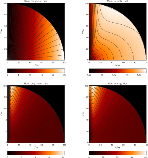
In Fig. 5, we show the results for a Poynting-flux-dominated flow (Case E), corresponding to a ratio ⁠, where the integration is again performed over 4π solid angle. In this case the solution is mostly magnetically driven, and plasma effects lead to small deviations with respect to the force-free limit.

Figure 5

Open in new tabDownload slide

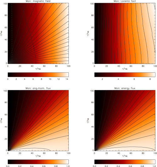
Results for the 2D monopole in the highly magnetized Case E (Table 3). Upper left-hand panel: contours represent poloidal magnetic field lines, while colours represent the ratio |B_φ/B_r|. The FM surface (dotted line) is more distant from the axis while the AL surface (dashed line) is very close to the Light Cylinder. Upper right-hand panel: colours and contours represent the Lorentz factor. There is no evidence here of the relatively slow channel on the axis as in Case A (see Fig. 4) and the Lorentz factor scales as sin (θ). Lower left-hand panel: angular momentum flux in non-dimensional units ⁠. Lower right-hand panel: total energy flux in non-dimensional units (see equations 23–27 for conversion in physical units). Here, these fluxes are higher at the equator than at the pole (compare with Fig. 4), as expected when the flow is relativistic and Poynting-flux-dominated.

Similar to the mass-loaded Case A, at the neutron star surface we find that the mass flux is higher at the equator than at the pole, and that the AL and FM surfaces are extended in the direction of the pole. Here, the FM and AL surfaces intersect the equatorial plane at a distance of 46r_NS (to be compared with 40.5 =σ^1/3₀R_L) and 6.7r_NS, respectively, while the SM surface is more spherical than Case A and intersects the pole and the equator at a distance of 2.5r_NS and 1.7r_NS, respectively. Magnetic field lines are again monopolar, but while in the mass-loaded Case A this was a consequence of a originally centrifugally driven wind, now this is due to electromagnetic force balance. The dynamics of a magnetized outflow are governed by the combination of Lorentz and Coulomb forces. In the relativistic regime the Coulomb force cannot be neglected and, as the flow speed approaches c, the Coulomb force balances the Lorentz force, suppressing collimation. As a consequence, the flux tubes in a Poynting-flux-dominated wind have an areal cross-section that scales as r². It is known that the efficiency of conversion of magnetic energy to kinetic energy increases when the flow divergence becomes more than radial (Daigne & Drenkhahn 2002). In the high-σ₀ simulation presented here, at least within the limited computational domain employed, we do not see evidence for efficient conversion and acceleration. As found by (Bogovalov 2001) there is evidence for a narrow collimated channel very close to the axis, but in our case, where the mass flux at the injection is not imposed, the mass flux in the channel is not strongly enhanced. However, the FM surface on the axis does not close in our computational box so no strong conclusion can be drawn.

The upper right-hand panel of Fig. 5 shows that the Lorentz factor in the wind scales approximately as sin θ. The maximum value achieved in the computational domain is 8. The latitude dependence is not appreciable, probably because our solution does not extend far enough away from the star. As in the 1D models, for the range of parameters investigated, the total mass flux from the star is not much affected by the value of the surface magnetic field. For the Poynting-flux-dominated Case E it is about three times higher than in the mass-loaded Case A, despite the fact that the magnetic energy density is 5000 times higher. This again follows from the fact that the AL surface is larger than the SM surface. However, there are important qualitative differences between Cases A and E. In Case E, we find that on large scales magnetic acceleration is dominant and the mass flux is maximal on the equator, instead of on the axis. In addition, the lower panels of Fig. 5 show that the energy and angular momentum fluxes increase toward the equatorial plane and are almost completely magnetically dominated. In fact, the energy and angular momentum loss rates scale as sin²θ, as expected in the force-free limit. This strong transition in the angular dependence of the energy and momentum fluxes, from strongly collimated to equatorial, occurs at σ₀∼ 1.

Fig. 6 shows the behaviour of the angular momentum and energy losses as σ₀ increases. We again observe the convergence to the force-free limit (see also Table 3) and recover the expected behaviour in the mass-loaded cases. The convergence to the force-free solution can be approximated, as in the 1D case, with a power law of the form C_o+C₁(1/σ₀)^β. The fits are different than the 1D models because the flux tubes deviate from being strictly monopolar. We find for the angular momentum loss rate ⁠, for the total energy losses ⁠, and for the reduced energy ⁠. As mentioned before, we have derived these fits within the parameter range of our simulations, and there is no guarantee that they can be extrapolated for much higher or lower magnetizations. We stress that in the highly magnetized Case E our results are very close to the force-free solution: (Michel 1991). Note also that such a value is lower than what would be expected from a trivial 2D extension of the 1D monopole (0.78 =⁠).

Figure 6

Open in new tabDownload slide

Loss rates for a 2D monopole in non-dimensional units. Upper panel: angular momentum loss rate. Lower panel: total energy-loss rate. Dashed curves represent the theoretical expectation for the losses in the mass loaded cases (Section 2.2) and ⁠. Continuous curves represent the best power-low fit given in the text. The dotted lines are the force-free limits. The square mark indicates Case B1, which has a different rotation rate (Table 1).

The efficiency of conversion of the magnetic energy to kinetic energy is maximal on the equator, but it does not exceed 10 per cent at the outer boundary. We note that conversion is faster than logarithmic in radius and at the edge of the computational box it scales as R^1/3, similar to our 1D results. However, we cannot draw strong conclusions on the terminal efficiency far outside of the FM surface because of the limited size of our computational domain. As shown by Bogovalov (2001), γ seems to increase after the FM point and then saturates at larger distances.

5.3 The aligned dipole

To lowest order, currents in the neutron star should generate a dipole magnetic field. This field configuration is much more realistic than the monopolar models considered in Sections 5.1 and 5.2. A dipole field may also have interesting consequences for the asymptotic character of the outflow. For example, it is possible that the presence of a closed zone, outside of which the open field lines at first expand much more rapidly than radially, might provide for a more efficient conversion of magnetic energy into kinetic energy, leading to a higher terminal Lorentz factor (Section 1). Below, we review several numerical issues associated with our dipole wind solutions and then we present our results, which again bridge the transition from low- to high-σ₀ outflows.

5.3.1 Numerical challenges

The modelling of a magnetic wind with a closed zone and an equatorial current sheet presents a number of numerical difficulties. We have encountered two problems in particular that bear mention. The first is that the outer edge of the closed zone rotates faster than what is required by equation (19). We believe this ‘supercorotation’ is connected with numerical dissipation in the equation for the evolution of B_φ and that it stems from the fact that the boundary between the closed and open field regions is not grid-aligned.4 By suppressing the upwinding term in the HLL flux we were able to reduce the deviation from the corotation condition from 10–20 per cent to ∼5 per cent, but at the price of making the code less stable when the flow is highly magnetized. Unfortunately, of the previous papers dealing with winds in the presence of a closed zone in the MHD regime, only Keppens & Goedbloed (2000) discuss deviations from corotation in the closed zone. In their paper these amount to ∼10–20 per cent, and they consider only parameters appropriate to the Sun, a slow rotator.

The second problem is that the magnetic field undergoes reconnection at the neutral current sheet on the equator close to the position of the Y-point, where the last closed field line intersects the equatorial plane. As a consequence, plasmoids are formed and advected away, thus preventing the system from reaching a steady-state configuration.5 At the current sheet B_r and B_φ change sign, the MHD approximation fails, and a sharp discontinuity develops that cannot be well resolved. Fig. 7 shows an example of plasmoid formation. Although it is well known that current sheets in the presence of a Y-type point are subject to reconnection and the continuous formation of plasmoids (Yin et al. 2000; Endeve & Leer 2003; Tanuma & Shibata 2005), in our case the high value of σ₀ does not allow us to properly resolve the current sheet. For this reason, the reconnection processes are dominated by the intrinsic numerical resistivity of our numerical scheme.

Figure 7

Open in new tabDownload slide

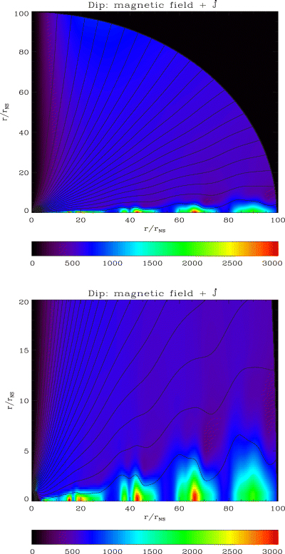
Magnetic structure of a magnetically dominated flow (Case C). The upper panel shows the poloidal magnetic field structure, with a snapshot of outflowing plasmoids forming along the equatorial current sheet outside the closed zone. The lower panel shows a blow up of these plasmoids, which travel out at close to the speed of light. The colour indicates the angular momentum density, with roughly 20 per cent of the angular momentum loss being carried by these intermittent structures. Values are in code units (equations 23–27). As stated in the text, the numerical values in the plasmoids depend on numerical resistivity.

We have found that the formation and growth of plasmoids depends on two terms in the definition of the HLL electric field (see equation 44 of Del Zanna et al. 2003): ∂B_r/∂θ and B_rv_θ. The first behaves like an explicit resistivity and seems responsible for the evolution of the plasmoids as they are advected off the grid along the equator. The second term behaves like forced reconnection and controls the initiation of plasmoid formation (given that the current sheet is not resolved, v_θ is not reconstructed to zero on the equator). Setting both terms to zero causes the closed zone to disappear entirely and the system evolves toward a modified split monopole. To deal with this issue and explicitly enforce a steady state, we opt for the following procedure: in a calculation with plasmoids we note the position of the Y-point and we then impose the conditions ∂B_r/∂θ= 0 and B_rv_θ= 0 on the equator outside the position of the Y-point as inferred from the calculation without these boundary conditions. The condition ∂B_r/∂θ= 0 can be justified because of the structure of the characteristic waves and because the solution should be symmetric about the equatorial plane. The equator is a contact discontinuity, so only the total pressure is important as a boundary conditions and not the sign of the parallel magnetic field, in fact for infinite conductivity a pure monopole and a split monopole have the same solution. The condition B_rv_θ= 0 corresponds to enforcing v_θ= 0.

We note that the steady state solution need not be the physically correct solution found in nature. The equatorial current sheet in the vicinity of a neutron star is undoubtedly dissipative, and is thus subject to reconnection and plasmoid formation. However, a full understanding of this behaviour requires – at the very least – the use of resistive RMHD, so that the dissipation can be controlled, rather than being fully numerical, as in our current calculations. Such a treatment is beyond the scope of this paper. Thus, we focus our attention here on the forced steady state solutions described above. As a test, we have compared the global energy and angular momentum loss rates between time-dependent calculations with plasmoids and those with our forced steady state boundary conditions outside the Y-point. In general, losses are higher in the latter calculations because the open magnetic flux is larger. In Case A the difference is less than 5 per cent, while in Case C it is about 15–20 per cent (see Table 4 and Fig. 8). In the time-dependent calculations the individual plasmoids represent fractional deviations in and from the average of up to 15 per cent in Case C, and less for lower σ₀ flows. Thus, the plasmoids do not appear to be that dynamically significant for the overall energy and angular momentum losses from the neutron star.

Table 4

Results of the dipole models.

Model .	σ0 .	.	.	.	rY/RL .
A	0.298	66	1.53	5.28	0.26
B2	1.34	7.8	0.965	1.81	0.32
B	2.77	43	0.853	1.27	0.37
B1	3.91	114	0.816	1.10	0.48
C	17.5	42	0.701	0.73	0.47

Model .	σ0 .	.	.	.	rY/RL .
A	0.298	66	1.53	5.28	0.26
B2	1.34	7.8	0.965	1.81	0.32
B	2.77	43	0.853	1.27	0.37
B1	3.91	114	0.816	1.10	0.48
C	17.5	42	0.701	0.73	0.47

⁠; ⁠; ⁠; and ⁠. Values are given in code units, see equations (23)–(27) for conversion to physical units. Cases B1 and B2 have different rotation rates (Table 1). All cases have ⁠.

Open in new tab

Table 4

Results of the dipole models.

Model .	σ0 .	.	.	.	rY/RL .
A	0.298	66	1.53	5.28	0.26
B2	1.34	7.8	0.965	1.81	0.32
B	2.77	43	0.853	1.27	0.37
B1	3.91	114	0.816	1.10	0.48
C	17.5	42	0.701	0.73	0.47

Model .	σ0 .	.	.	.	rY/RL .
A	0.298	66	1.53	5.28	0.26
B2	1.34	7.8	0.965	1.81	0.32
B	2.77	43	0.853	1.27	0.37
B1	3.91	114	0.816	1.10	0.48
C	17.5	42	0.701	0.73	0.47

⁠; ⁠; ⁠; and ⁠. Values are given in code units, see equations (23)–(27) for conversion to physical units. Cases B1 and B2 have different rotation rates (Table 1). All cases have ⁠.

Open in new tab

Figure 8

Open in new tabDownload slide

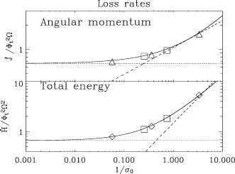
Loss rates for a 2D dipole in non-dimensional units. Upper panel: angular momentum loss rate. Lower panel: total energy-loss rate. Dashed curves represent the theoretical expectation for the losses in the mass loaded cases and ⁠. Continuous curves represent the best power-law fit of the 2D monopole of Fig. 6. The dotted lines are the force-free solution. The squares mark cases B1 and B2, which have different rotation rates (see Table 1).

5.3.2 Results

In Table 4, we show the results of our simulations using the prescription described above. In the monopole models the magnetic field lines are open so that normalizing to the surface magnetic field or to the total magnetic flux Φ_t is equivalent. In the dipole case, because of the closed zone, the two quantities are not proportional. We find it useful to normalize in terms of the magnetic flux evaluated on open field lines, Φ_o, where equations (17)–(22) hold. As a consequence, we can define an equivalent surface magnetic field B_r-equiv(r_in) as the surface magnetic field of a monopole that has the same amount of open magnetic flux. Contrary to the monopole case, increasing the magnetic field strength at the stellar surface reduces the mass-loss rate because the size of the closed zone increases. Similarly, for the parameters explored here, an increase in the magnetic field strength by a factor of, say, ∼3 at the stellar surface leads to an increase in the open magnetic flux Φ_t by a factor of just ∼2.5, rather than the one-to-one behaviour for the monopole. We can derive an approximate relation between the magnetic field at the pole on the surface of the star (r_NS), and the equivalent surface magnetic field, that can easily be computed if and Ω are known. We find that in all our cases the relation is

28

Thus, the problem of relating the surface magnetic field to the loss rates is reduced to the problem of determining the size of the closed zone.

In Fig. 8, the angular momentum and energy-loss rates are plotted. The continuous lines in this figure are not a fit to our dipole results, but are simply the same curves as in Fig. 6 for the 2D monopole. In addition, as in Fig. 6, the dashed lines are the analytic expectation for the loss rates in the mass-loaded limit for the monopole (Section 2.2). This shows that if the solutions are parametrized in terms of the open magnetic flux, then the dipole and monopole winds have very similar behaviour within the parameter space we have investigated. This can be easily understood if one considers the structure of the outflow in the far region. Given that and are integrals, they can be evaluated at any distance from the star. Even if the field is dipolar close to the star it is nearly monopolar outside R_L. Even when we do not impose our steady-state boundary conditions at the equator, and plasmoids are present during the evolution, and closely follow our results for the monopole (again, as long as these losses are written in terms of the open magnetic flux). Note also that in Fig. 8, we find that and converge to the expected value of 2/3 in the force-free limit (Contopoulos et al. 1999; Gruzinov 2005). However, as we discuss below, r_Y < R_L in all of our calculations, contrary to the assumption that r_Y=R_L in the above force-free treatments.

We can extrapolate our results to the force-free limit for the spindown rate. In terms of the equivalent surface magnetic field, and using equation (28) with r_Y=R_L and B_o= 0.5B_r(r_NS, θ= 0) we have

29

in agreement with Gruzinov (2005).

The flow structure for both low σ₀ (Case A) and high σ₀ (Case C) are shown in Fig. 9. These figures show that the poloidal magnetic field for R > R_L has a structure very similar to that obtained from the monopole calculations. Also, B_φ scales as sin θ, except in a region close to the equatorial plane where it changes sign. This agrees with the results of Fig. 8 showing that the energy and angular momentum losses scale as for a monopole.

Figure 9

Open in new tabDownload slide

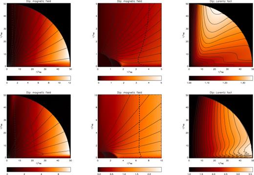
Result of the 2D dipole. Upper panels represent Case A, lower panels Case C. Left-hand panel: contours represents poloidal magnetic field lines, while colours represent the ratio B_φ/B_r. The dotted line is the FM surface, the dashed line the AL surface. In Case C the AL surface is close to R_L. Middle panel: contours represents poloidal magnetic field lines, while colours represent the ratio B_φ/B_r, in a region closer to the star. Now the dotted line represents the SM surface. Right-hand panel: colours and contour represent the Lorentz factor.

As expected, we find that the size of the closed region increases with magnetization. The position of the Y-point moves from 1.8r_NS in Case A, to 2.5r_NS in Case B, to 3.1r_NS in Case C. Thus, an increase in σ₀ of a factor of ∼60 corresponds to a ∼70 per cent increase in the size of the closed zone. Importantly, even at relatively high σ₀ (∼18 for Case C), these values are significantly smaller than the Light Cylinder radius R_L= 6.8r_NS. In order to understand the systematics of the Y-point, we have calculated several models with different rotation rates Ω (see Tables 1 and 4). The radius of the Y-point changes from 2.2r_NS in Case B1, to 2.5r_NS in Case B, to 4.3 r_NS in Case B2. Although r_Y is largest in the model with slowest rotation (Case B2), this model has the smallest ratio r_Y/R_L. Indeed, we find that r_Y/R_L decreases as Ω decreases. This trend yields a braking index less than 3. If one takes Cases B1, B and B2 as a time-series in the life of a neutron star, one would infer a braking index ∼2.2.

In general, the size of the closed zone will depend on the physical conditions at the stellar surface, including the thermal sound speed and the mass density, which govern the mass-loss rate on each open streamline (see Section 2.1; Mestel & Spruit 1987). This shows that even a small thermal pressure can have an important effect on the torque. Fig. 9 shows that in Case A both the AL and the FM surfaces are inside the radius of the Light Cylinder. However, in the high-σ₀ Case C the AL surface is very close to R_L. This suggests that although the AL surface rapidly approaches R_L as σ₀ increases, the position of the Y-point remains inside R_L and is a weak function of σ₀. It is thus possible to produce a relativistic outflow, even if the Y-point is well inside R_L. Because the range of parameters we have explored is fairly limited, we can only conclude that quite large magnetization is required to achieve r_Y=R_L. A rough extrapolation of our results implies that B_r(r_in, θ= 0)²/ρ(r_in) must be of order 10⁵–10⁶ to achieve r_Y≈R_L, but at the moment we deem premature to draw strong conclusions.

We stress here that the magnetization parameter σ₀ is defined as an integral average. It is known that in a dipolar field geometry with sub-SM injection, the mass flux at the edge of the closed zone is higher than the average integrated value over the entire star (Kopp & Holzer 1976). Thus, the magnetization varies from high to low latitudes. For example, in our Case C the magnetization on the open flux tubes immediately adjacent to the closed zone is less than 7, while the σ₀ parameter for this model is 17.5. Because the position of the Y-point and the shape of the magnetosphere depend on local equilibrium between the closed and open zones, this strong variation in magnetization in latitude may help explain why even if the global flow has σ₀≫ 1, r_Y is less than R_L.

The upper and lower far right-hand panels of Fig. 9 show that for the Lorentz factor we recover similar behaviour as for the monopole (compare with Figs 4 and 5). In Case A, the Lorentz factor reaches its maximum at about 70° from the equator. We also notice that there is now a slower equatorial flow corresponding to what is known as the ‘slow solar wind’ in models of the Sun's outflow. In Case C the Lorentz factor appears to scale mostly as the cylindrical radius. This again was found for the monopole. The slow-wind region is still present, but now the boundary conditions we have imposed on the equator to suppress the plasmoids cause a noisy structure in v_r.

The shape of the field lines outside the FM surface does show significant differences between the monopole and the dipole. In the dipolar Case C at r= 50r_NS the maximum value of B_θ/B_r=−0.06. Such a value for this ratio is in between Cases C (−0.08) and D (−0.03) for the 2D monopole. Our limited computational domain prohibits a more quantitative study of the poloidal field line shape at still larger distances from the neutron star.

Lastly, the angular distribution of the energy and momentum loss rates in our dipole models are qualitatively similar to those we obtained for the 2D monopole (see the bottom panels of Figs 4 and 5). For low-σ₀ outflows, because of hoop stress, and far from the neutron star are peaked at high latitudes, along the axis of rotation. In contrast, for high-σ₀ outflows, and are maximum near the equator, similar to Fig. 5 (Case E).

6 DISCUSSION AND CONCLUSIONS

We have solved for the dynamics of time-dependent relativistic MHD winds from rotating neutron stars, including the effects of general relativity on the gravitational force. The mass-loss rate along open field lines is derived self-consistently as a solution to the RMHD equations, subject to the boundary conditions at the stellar surface (finite thermal pressure) and a polytropic equation of state. We consider 1D and 2D monopole field geometries and the aligned dipole, and we explore solutions that cover the parameter regime from non-relativistic mass-loaded low-σ₀ outflows to relativistic Poynting-flux-dominated high-σ₀ outflows. Our primary results are

• (i)

  In the 1D and 2D monopole calculations, we reproduce the expected analytic trends in both the high- and low-σ₀ limits. In particular, the solutions asymptotically approach the force-free limit when σ₀≫ 1.

• (ii)

  In both the dipole and 2D monopole solutions, when σ₀ < 1, the energy and momentum losses far from the neutron star are highly directed along the axis of rotation. The zenith angle at which these fluxes are maximized is an increasing function of σ₀ so that for σ₀ > 1, the losses are primarily equatorial.

• (iii)

  In both the dipole and 2D monopole solutions, for winds with σ₀ < 1, the Lorentz factor peaks at high latitudes.

• (iv)

  For the aligned dipole, the equatorial current sheet may be unstable to the formation of plasmoids, leading to time-dependent spindown of the neutron star. A proper treatment of dissipative RMHD in the equatorial region is needed to explore this issue more completely.

• (v)

  If the energy and angular momentum losses from the aligned dipole are parametrized in terms of the open magnetic flux, then the results are nearly identical to those from the 2D monopole solutions in both the mass-loaded and Poynting flux-dominated regimes. In particular, the dipole calculations quantitatively approach the force-free limit when σ₀≫ 1. The normalization for the angular momentum loss rate is k≈ 24/25 (equation 29), in good agreement with the force-free results found by Gruzinov (2005) and Spitkovsky (2006).

• (vi)

  For average integrated magnetization parameters as high as σ₀≈ 20, the radial position of the Y-point (r_Y), which bounds the closed zone in the dipole models, is significantly less than the Light Cylinder distance. This result obtains despite the fact that the AL point rapidly approaches R_L for σ > 1. The ratio r_Y/R_L is a very slowly increasing function of the surface magnetic field strength. An extrapolation of our results indicates that σ₀ must be very large, σ₀≫ 100, for the Y-point to reach the Light Cylinder. That r_Y is generically much less than R_L in our calculations is due in part to the fact that although σ₀≈ 20 globally (Case C, Section 5.3) the magnetization along the open field lines nearest the closed zone is less than 7.

• (vii)

  Over limited dynamic range, the ratio r_Y/R_L decreases as ω decreases in the dipole models. This behaviour is consistent with a braking index less than 3 (see Sections 2.1 and 6.1).

Concerning the acceleration of the wind, we do not find any evidence for efficient magnetic to kinetic energy conversion. However, we want to stress again that our computational box does not extend far enough from the star to appreciably probe the asymptotic behaviour of the wind.

6.1 Rotation-powered pulsars

Our results have several possible implications for rotation-powered pulsars, where σ₀ is high. The fact that the Y-point is interior to the Light Cylinder (and the Alfven radius) suggests that observed braking indices less than 3 might be a consequence of equilibrium magnetospheric structure. We emphasize that the position of the Y-point depends on a local equilibrium between the surface of the closed zone and the wind region. As a consequence, the value of the mass flux along the open field lines closest to the closed zone directly affects the position of the Y-point. The mass flux, in turn, depends on the boundary conditions at the stellar surface. In our simulations, the mass-loss rate is derived self-consistently, subject to a finite thermal pressure at r_NS. In the case of a pulsar, the injection of matter at r_NS is thought to be due to non-MHD pair creation processes (Hibschman & Arons 2001) in a ‘gap’ just above the stellar surface which, in an otherwise MHD flow, act to inject plasma with velocity already exceeding the sound speed. Then the mass-loss rate is determined by the gap physics, not by the requirement of making a smooth transition from subsonic to supersonic flow. Thus, in principle r_Y depends upon the injection law determined by the pair creation physics at the surface. For this reason, we caution against overinterpreting our results (vi) and (vii) in the pulsar context. Indeed, thermal pressure of the magnitude employed here is not likely to be relevant for classical pulsars.6 On the other hand, magnetic dissipation and reconnection at and near the Y-point might cause pressure and inertial forces to be significant in this localized region. In any case, our primary conclusions, that r_Y/R_L is generally less than unity and that r_Y/R_L decreases as Ω decreases, are intriguing possibilities now open to investigation with the advent of dynamical, large σ models of neutron star magnetopsheres. A more general study of the effect of the injection conditions on the structure of the magnetosphere and the accompanying wind is under way.7

The appearance of outwardly propagating plasmoids at and beyond the Y-point as a consequence of (numerical) magnetic dissipation raises the intriguing possibility that noise in pulsar spindown (Cordes & Helfand 1980) might arise from instability of the magnetospheric currents due to real magnetic dissipation (e.g. via the collisionless tearing instability). Our results show the possibility of 20 per cent or more torque fluctuations that could in principle give rise to a random walk in the rotation frequencies of pulsars, as is observed. Likewise, such torque fluctuations might give rise to noise and limit cycles in the observed phase of the subpulses of pulsars, as is seen in many systems (Rankin 1986; Deshpandhe & Rankin 1999). Determining whether these observed phenomena could be due to magnetospheric dissipation requires treating the dissipation with a consistent physical model, which is an investigation beyond that reported in this paper.

6.2 Proto-neutron stars and proto-magnetars

High thermal pressure at the neutron star surface is thought to be a generic feature of neutron star birth and so the calculations presented in this paper are directly relevant to young neutron stars, particularly in the hypothesized rapidly rotating and highly magnetic initial state of magnetars.

We identify five separate phases in the life of any very young neutron star: (1) a pressure-dominated essentially non-magnetic phase in which the wind is driven by neutrino-heating (as in e.g. Qian & Woosley 1996); (2) a phase in which magnetic field effects are present, but not dominant so that r_Aω < 0.1c≈c_T, where c_T is the isothermal sound speed at the proto-neutron star surface; (3) a non-relativistic magnetically dominated phase when R_A is greater than r_NS, but less than R_L; (4) a relativistic phase in which R_A∼R_L, but r_Y < R_L, and lastly (5) an epoch when the force-free limit is applicable and r_Y≃R_A≃R_L. Phases (1)–(5) represent a time evolution starting immediately after the supernova explosion commences. The time-scale for the evolution from phase (1) to phase (4) is set by the Kelvin–Helmholtz time-scale for cooling of the proto-neutron star, τ_KH∼ 10–100 s. The transition from phase (4) to phase (5) may occur on a longer time-scale, or not at all, depending upon the applicability of our results to classical pulsars as the MHD approximation breaks down.

For parameters appropriate to a proto-magnetar, phase (3) lasts of the order of τ_KH. Our simulations show that in this phase, the wind is energetic and that the energetic flux is highly directed along the axis of rotation. The characteristic rotational energy-loss rate in this phase is ⁠, where B₁₄=B(r_NS)/10¹⁴ G is the ‘equivalent’ monopole field (equation 28), and P₁=P/1 ms. On the time-scale τ_KH, the total amount of energy extracted is comparable to the asymptotic supernova energy, ∼10⁵¹ erg. The magnitude of the rotational energy extracted in this phase and its collimation along the rotational axis should have profound implications both for the spindown of millisecond magnetars and for the supernova remnants that accompany their birth. We save a detailed discussion for a future paper.

We thank Prof S. S. Komissarov, for providing us with a wave based Riemann solver, to verify effects of numerical diffusion in our 2D dipole calculations. Part of this work was done while N. B. and J. A. were in residence at the Kavli Institute for Theoretical Physics, with partial support from NSF Grant No. PHY99-07949. NB and JA were also supported in part by NASA grants TM4-5000X and NAG5-12031, and by NSF grant AST-0507813 to the University of California, Berkeley. EQ was supported in part by the David and Lucile Packard Foundation. TAT was supported during most of this work by NASA through Hubble Fellowship grant #HST-HF-01157.01-A awarded by the Space Telescope Science Institute, operated by the Association of Universities for Research in Astronomy, Inc., for NASA, under contract NAS 5-26555.

REFERENCES

Appendix

APPENDIX A: PARAMETRIZATION OF THE MODELS

All the simulations can be parametrized in terms of the ratios of characteristic velocities at the injection radius (r_in), see Table A1. Following the work by Mestel (1968a) and Goldreich & Julian (1970), these are essentially the sound speed c_T, the rotational velocity v_φ, the non relativistic AL velocity ⁠, and the escape speed ⁠. For the 2D cases we consider the value of the rotational velocity and the magnetic field at the equator. Note that the characteristic velocities defined above do not coincide with the cited works in Newtonian gravity. For example, the escape speed differs by a factor of ⁠, and in the definition of v_φ one must include the effect of time delay. These are corrections due to the general relativistic metric which are not present in the above cited papers (α(r_in) = 0.79).

Table A1

Parametrization of the numerical models.

Model .	Parameters .
1D model	A0	A	B	C	D	E	F	G	H	I
	11.44	11.44	6.74	7.54	8.98	10.45	11.44	6.29	6.29	6.29
	0.061	0.61	0.71	0.80	0.95	1.11	60.6	133	533	1330
	9.43	9.43	9.43	9.43	9.43	9.43	9.43	9.43	9.43	9.43
2D monopolar model	A	B	B1	C	D	E
	11.44	11.44	11.44	11.44	11.44	11.44
	0.61	6.1	6.1	60.6	606	3030
	9.43	9.43	4.20	9.43	9.43	9.43
2D dipolar model	A	B	B1	B2	C
	11.44	11.44	11.44	11.44	11.44
	1.22	12.2	12.2	12.2	122
	9.43	9.43	4.20	38.5	9.43

Model .	Parameters .
1D model	A0	A	B	C	D	E	F	G	H	I
	11.44	11.44	6.74	7.54	8.98	10.45	11.44	6.29	6.29	6.29
	0.061	0.61	0.71	0.80	0.95	1.11	60.6	133	533	1330
	9.43	9.43	9.43	9.43	9.43	9.43	9.43	9.43	9.43	9.43
2D monopolar model	A	B	B1	C	D	E
	11.44	11.44	11.44	11.44	11.44	11.44
	0.61	6.1	6.1	60.6	606	3030
	9.43	9.43	4.20	9.43	9.43	9.43
2D dipolar model	A	B	B1	B2	C
	11.44	11.44	11.44	11.44	11.44
	1.22	12.2	12.2	12.2	122
	9.43	9.43	4.20	38.5	9.43

Open in new tab

Table A1

Parametrization of the numerical models.

Model .	Parameters .
1D model	A0	A	B	C	D	E	F	G	H	I
	11.44	11.44	6.74	7.54	8.98	10.45	11.44	6.29	6.29	6.29
	0.061	0.61	0.71	0.80	0.95	1.11	60.6	133	533	1330
	9.43	9.43	9.43	9.43	9.43	9.43	9.43	9.43	9.43	9.43
2D monopolar model	A	B	B1	C	D	E
	11.44	11.44	11.44	11.44	11.44	11.44
	0.61	6.1	6.1	60.6	606	3030
	9.43	9.43	4.20	9.43	9.43	9.43
2D dipolar model	A	B	B1	B2	C
	11.44	11.44	11.44	11.44	11.44
	1.22	12.2	12.2	12.2	122
	9.43	9.43	4.20	38.5	9.43

Model .	Parameters .
1D model	A0	A	B	C	D	E	F	G	H	I
	11.44	11.44	6.74	7.54	8.98	10.45	11.44	6.29	6.29	6.29
	0.061	0.61	0.71	0.80	0.95	1.11	60.6	133	533	1330
	9.43	9.43	9.43	9.43	9.43	9.43	9.43	9.43	9.43	9.43
2D monopolar model	A	B	B1	C	D	E
	11.44	11.44	11.44	11.44	11.44	11.44
	0.61	6.1	6.1	60.6	606	3030
	9.43	9.43	4.20	9.43	9.43	9.43
2D dipolar model	A	B	B1	B2	C
	11.44	11.44	11.44	11.44	11.44
	1.22	12.2	12.2	12.2	122
	9.43	9.43	4.20	38.5	9.43

Open in new tab

Notice that for the dipole, where the open field lines originate close to the pole, the base value of the magnetic field is about twice stronger than at the equator, and the rotational velocity is much smaller than the equatorial speed.

Footnotes

Author notes