


Abstract
Concurrent physical, chemical and biological observations across the Kuroshio Front collected in October 2009 provide a detailed view of the relationship between the physical environment and the phytoplankton community. Depth profiles were taken at stations ∼9 km apart along five 70 km transects. With a combination of flow cytometry, microscopy and high-pressure liquid chromatography pigment analysis, we characterized the phytoplankton community structure across the front. The observed phytoplankton community fell into two distinct assemblages, largely separated by the front, but which also reflected patterns in the distribution of Kuroshio and Oyashio water masses shaped by mesoscale lateral mixing. Phytoplankton biomass was elevated where there was a positive vertical flux of nitrate towards the surface, and the frontal circulation drove a lateral transport of nutrients southwards into the subtropical gyre. The observations showed that the phytoplankton respond to forcing on several scales: the phytoplankton community across the front was shaped by a combination of the large scale biogeography of the region, mesoscale mixing of populations and finer scale modification of the light and nutrient environment.
INTRODUCTION
Phytoplankton growth and loss processes act on time scales of days and can be strongly modulated by horizontal and vertical motions associated with oceanic fronts. Fronts are important and ubiquitous dynamical features and are known to be sites of high biological productivity (Yoder et al., 1994). Frontal circulations generate vigorous vertical motions (Pollard and Regier, 1990; Rudnick and Luyten, 1996) which are important in setting the supply of inorganic nutrients from below the mixed layer, and in modulating the light environment for phototrophic cells. Although small compared with the scale of ocean basins, the effect of frontal features is likely to be important when integrated over the whole basin (Follows and Marshall, 1994) and the link between these dynamic features and phytoplankton growth and community structure deserves closer study. However, observations of patterns of phytoplankton assemblages at the scale of these physical features are rare.
The phytoplankton community structure observed across a front results from a combination of physical and biological processes spanning several orders of magnitude in space and time scales. We may conceptually divide these into ‘local’ interactions, where frontal scale motions drive ecosystem responses on time scales of hours, and ‘remote’ forcing, associated with along-front transport on scales of hundreds of kilometres and timescales of weeks or more. The distinct character of the phytoplankton assemblage changes abruptly across a front, from the stable, subtropical waters to the highly seasonal subpolar gyres. The large-scale convergence of subtropical and subpolar water masses at a front brings subtropical and subpolar biomes into close proximity but the strong density gradient at the front also acts as a barrier in the surface ocean (Bower et al., 1985; Bower and Lozier, 1994) maintaining the ecological gradient. Instability of the front, however, leads to the formation of rings and exchange of physical, chemical and biological properties across the front, potentially enhancing local diversity and mingling biomes (Clayton et al., 2013).
Coastal species have been observed within the main stream of both the Gulf Stream (Lillibridge et al., 1990) and the Kuroshio (Yamamoto et al., 1988). The stream itself acts as a ‘river’ transporting subtropical waters, along with their distinct physical, chemical and ecological properties, far from their point of origin. Subtropical species have been observed in large numbers in the core of the Gulf Stream (Cavender-Bares et al., 2001), likely due to this transport mechanism. Whether immigrant populations can continue to actively grow, or are excluded as they transported away from their point of origin depends on the modulation of their environment by local processes. These act on time scales of a few days on a length scale set by the cross frontal distance, and include large intermittent nutrient fluxes driven by the ageostrophic vertical circulation as well as strong mixing events associated with wave generation and instabilities at the front (Nagai et al., 2012). These may fuel primary production by increasing upwards transport of nutrients, or entrain phytoplankton cells more quickly than they can photo-acclimate (Nagai et al, 2003; Falkowski and Raven, 2007) which could have a negative effect on primary production. Opportunistic phytoplankton groups (e.g. diatoms) with fast population growth are better adapted to variable environmental conditions (Margalef, 1968; Grover and Chrzanowski, 2004), and might be more competitive in regions of the front where local processes create a highly variable environment. However, the biological response to physical forcing in frontal zones may lag by as much as several days (Yamazaki et al., 2009), making it hard to distinguish between the effects of fast-acting local processes, and slower remote processes on the phytoplankton community structure.
The Kuroshio Extension Front is an intense front with zonal velocities O (1 m s−1), and where turbulent dissipation and mixing can be enhanced in the surface boundary layer (D'Asaro et al., 2011; Nagai et al., 2012) by down-front wind stress (Thomas and Lee, 2005) and in the thermocline (Kaneko et al., 2012; Nagai et al., 2012). Recent observations in similarly dynamic regions reveal richness in biological and physical structure on lateral scales ranging from meters to kilometers (D'Ovidio et al., 2010; Ribalet et al., 2010). Most previous studies of the Kuroshio and Western North Pacific have described the diversity and distribution of microbial and planktonic species at the large scale, finding a shift in the dominant phytoplankton group between subtropical Kuroshio and subpolar Oyashio water masses (Odate et al., 1990; Kataoka et al., 2009). However, these observations, made at intervals of more than 1° of latitude, effectively miss any fine scale variability associated with the Kuroshio Front itself. Yamamoto et al. (Yamamoto et al., 1988) conducted a series of three high-resolution (<2 km between stations) surveys of phytoplankton along short transects (∼20 km) across the Kuroshio Front and observed fine scale variations in diatom and dinoflagellate distributions. They found that the phytoplankton community could be separated into subtropical and subpolar assemblages found either side of the front, and that a distinct group, including coastal diatoms, was present at the core of the stream. However, there was no vertical information in that study, although the vigorous frontal circulations may have an important impact on the population and productivity. To date, the distribution of the pico-phytoplankton, important contributors to oceanic primary production (Marañón et al., 2001), has not been characterized in the Kuroshio Front.
Here, we provide a new view of the Kuroshio system, with a coordinated horizontal and vertical sampling of the phytoplankton on relatively fine scales, spanning the full size and taxonomic range of phytoplankton. We characterize the spatial distribution of phytoplankton along two sections across the Kuroshio Extension Front, sampled in October 2009. We use a range of complementary methods to characterize the phytoplankton community: flow cytometry, microscopy and pigment analysis by high-pressure liquid chromatography (HPLC). We examine the ratio of photosynthetic and photoprotective carotenoids (PPC) to chlorophyll to understand the physiological response of the phytoplankton community to vertical mixing and the light environment in the frontal zone. We place these observations in context with concurrent sampling of inorganic nutrients and hydrography, and discuss how both local and remote controls on the phytoplankton community act to shape the observed distributions.
METHOD
Cruise outline
Observations were made along five north–south transects across the Kuroshio Extension during a cruise aboard the R/V Natsushima (JAMSTEC), 17–24 October 2009. The transects were labelled A–E from west to east (Fig. 1A). Samples were collected at eight stations roughly 9 km apart along each transect. At each station, samples were recovered from five depths, including the sea surface. Water column samples were obtained using 2 L Niskin bottles mounted on a rosette sampler along with the CTD (Advantech Ltd.) and Lowered Acoustic Doppler Profiler (L-ADCP, 300 kHz). Surface samples were obtained with a clean plastic bucket. In addition, XBTs were deployed at 12 stations every 11.1 km along each transect providing temperature data north and south of the CTD stations. The physical oceanographic features of the study region during this cruise are described in detail in Nagai et al. (Nagai et al., 2012). Relevant details are briefly summarized below.
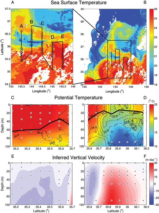
Physical setting of the study area. (A) Sea surface temperature for the study area on 21 October 2009. The cruise track is overlain with a solid black line, and the open circles show the location of CTD stations. (B) Sea surface temperature of the larger region showing the presence of a warm filament coiled to the north of the Kuroshio Front. Temperature sections, with salinity indicated by black contour lines for transect E (C) and transect D (D). Black circles show the depths sampled along each transect, and the mixed layer depth (defined as the depth where the density is 0.125 kg m−3 higher than at the surface) is shown as a thick black line. Vertical velocities (m day−1) inferred using the ω-equation (Nagai et al., 2012) for transect E (E) and transect D (F).
We collected samples along all transects, but restrict our analysis to the final two sections, D and E, for which we have a complete set of chemical and biological analyses. On each transect, we sampled part of the high velocity core of the Kuroshio current. Transect D is offset to the north of the front, whereas transect E is offset to the south (Fig. 1A). Thus we have observations from both the subtropical Kuroshio water south of the front, and the colder Oyashio and mixed waters found to the north. Kuroshio water is typically saltier with a characteristic salinity, S>34.2, whereas Oyashio water is fresher with S <33.5 (Qiu, 2001). Transect E is dominated by Kuroshio water, while transect D passes through a parcel of cooler and fresher Oyashio water at the surface just north the core of the stream. The mixed layer depth ranges from ∼60 m at the southernmost edge of transect E to 20 m at the northernmost edge of transect D, with a very sharp transition at the front (Fig. 1C and D). A filament of subtropical Kuroshio water is coiled to the north of the Oyashio water parcel at the northern extent of the transect. This warm filament is shown very clearly in sea surface temperature at the time of the cruise (Fig. 1B). Similar features are often observed in this region (Kawai and Saitoh, 1986). Intrusions of Oyashio water into the frontal region have been observed in previous studies of this region (Yamamoto et al, 1988) and may play an important role in entraining nutrients and plankton.
Nagai et al. (Nagai et al., 2012) calculated the inferred mesoscale vertical velocities along these two sections (Fig. 1E and F), using the QG ω-equation, indicating an upwelling tendency north of the front, and downwelling to the south. This pattern of vertical velocities is expected given that the front was transitioning from a meander trough in transect D to a meander crest from in transect E (Nagai et al., 2012). We note that the Rossby number is large in this region and the vertical velocities indicated using the QG ω-equation provide an indication of the patterns of mesoscale upwelling and downwelling, but not an accurate description of the vertical velocities.
Picoplankton analysis by flow cytometry
We followed the protocol outlined in Malmstrom et al. (Malmstrom et al., 2010) for sample collection and analysis. Whole seawater samples were collected and immediately fixed with gluteraldehyde (at a final concentration of 0.125% v/v), kept in the dark for 10 min, frozen in liquid nitrogen and stored at −80°C until they could be analysed. Analysis was conducted on a Cytopeia Influx flow cytometer. Prochlorococcus, Synechococcus and picoeukaryote populations were identified and quantified based on their unique autofluorescence and scatter signals (Olson et al., 1990a, b), using FlowJo software (Tree Star, Inc., www.flowjo.com).
Microscopic analysis of nano- and microplankton
We collected 500 mL of whole seawater from each depth and fixed it with buffered formalin (at a final concentration of 2% v/v). The identification of the micro-phytoplankton by microscopy was conducted by commercial analysts, PlantBio (www.plantbio.com). PlantBio followed the Sukhanova (Sukhanova, 1978) protocol for settling seawater samples prior to subsampling and microscope identification. They provided cell counts for each station/depth for species identified, organized by group for diatoms, dinoflagellates and silicoflagellates. Total cell numbers were provided for groups of smaller phytoplankton (haptophytes, prasinophytes and euglenophytes), but they were not identified further.
HPLC analysis
Whole seawater was filtered onto 25 mm Whatman GF/F filters that were then frozen at −80°C until they could be analysed. The samples were analysed by the Horn Point Marine Laboratory at the University of Maryland for HPLC analysis following standard protocols (Hooker et al., 2005) Concentrations of a full suite of chlorophylls and carotenoids, listed in Table I, were determined.
Names, abbreviations and taxonomic designations for the phytoplankton marker pigments which were measured by HPLC (Jeffrey et al., 2005)
| Symbol | Pigment | Designation |
|---|---|---|
| Chla | Chlorophyll a | |
| Chlb | Chlorophyll b | Chlorophytes |
| DVChla | Divinyl chlorophyll a | Prochlorophytes |
| Allo | Alloxanthin | Cryptophytes |
| But | 19′-butanoxyloxyfucoxanthin | Haptophytes |
| Caro | Carotenes | |
| Diad | Diadinoxanthin | |
| Diat | Diatoxanthin | |
| Fuco | Fucoxanthin | Diatoms |
| Hex | 19′-hexanoyloxyfucoxanthin | Haptophytes |
| Peri | Peridinin | Dinoflagellates |
| Zea | Zeaxanthin | Cyanophytes and prochlorophytes |
| TChla | Total Chlorophyll a | Chla + DVChla |
| PPC | Photoprotective carotenoids | Allo + Caro + Diad + Diato + Zea |
| PSC | Photosynthetic carotenoids | But + Fuco + Hex + Peri |
Dissolved nutrients
Whole seawater was collected from each sample depth, filtered with 25 mm Whatman GF/F filters, collected into 50 mL plastic bottles and stored frozen at −20°C until analysis. Samples were analysed by the Water Quality Analysis Laboratory at the University of New Hampshire, where samples were analysed for NO2 + NO3, PO4 and SiO2 with standard wet chemistry methods (Gordon et al., 1993).
Data analysis and mapping
We used the DIVA gridding option in Ocean Data View (ODV4) (Schlitzer, 2012) to interpolate the biological and chemical data in space. MATLAB (The MathWorks Inc, 2010) was used for all other data analysis, and to produce the final plots of the interpolated fields.
All of the data from this cruise for the above analyses has been submitted to, and is freely available from the PANGAEA data repository (doi:10.1594/PANGAEA.819110).
RESULTS
Transects D and E were each offset relative to the core of the stream and are presented side-by-side, south to north (transect E to transect D), providing a quasi-continuous, overlapping view of properties across the front. Concentrations of NO2 + NO3 (Fig. 2, top panels) were higher in the surface mixed layer to the north of the front (transect D) than to the south (transect E). The nutricline shoals from ∼ 80 m to the south of the front to ∼50 m to the north. There was a pronounced doming upward of the nutricline at the core of the front in both transects, reaching 40 m at 35.9°N in transect D and 70 m at the northern most edge of transect E. The distributions of PO4 and SiO2 follow that of NO2 + NO3 very closely.
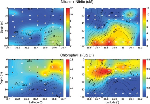
Sections of the concentration of, from top to bottom, nitrate + nitrite (μM) and chlorophyll a (μg L−1). Solid black lines define σt contours.
Inorganic nutrients and chlorophyll
The broad-scale frontal structure in the nutrient distributions was overlain by significant, finer-scale variability reflecting the vigorous mesoscale and submesoscale motions in the vicinity. Most notably, on transect E, there is a tongue in the concentrations of NO2 + NO3 (also present in PO4 and SiO2) at 60 m, extending from 35.25°N to 35.35°N. This causes an unusual inversion in the vertical profiles of nutrients, with concentrations of NO2 + NO3 of ∼3 μM within the tongue, but 1–1.5 μM above and below. The nutrient tongue was located in the density (σt) class 23–23.5 kg m−3 and was resolved by several samples. A similar, but less pronounced, feature was suggested by the data at the northern edge of transect D, at about 20 m, though only resolved by a single station.
Chlorophyll a was elevated at the core of the front (Fig. 2, bottom panels) with maximal concentrations of ∼0.63 μg L−1 on the southern edge of transect D abutting the southern side of the domed nutricline. Concentrations reached ∼0.55 μg L−1 at the northernmost edge of transect E. High chlorophyll a concentrations extended to the surface at the core of the front, where isopycnals outcrop, and extend southwards along transect E to at least 35.25°N; high chlorophyll a concentrations persist deeper in the water column to the limit of the transect at 35.15°N. Chlorophyll a was much patchier to the north of the front along transect D. Elevated concentrations persist to the northernmost edge of the transect in the uppermost 60 m of the water column. Below the 25 kg m−3σt surface, chlorophyll a declined to very low concentrations.
In order to explore the role of vertical transport of nutrients in stimulating production at the front, we estimated the mesoscale advective vertical flux of NO2 + NO3 (w(NO2 + NO3)) at a depth of 60 m (the approximate deepest horizon for chlorophyll) using vertical velocities inferred by Nagai et al. (Nagai et al., 2012) using the QG ω-equation (Fig. 3). Though there are errors associated with the application of QG in a high Rossby number regime, the analysis provides an indication of patterns in the vertical nutrient fluxes and their relationship to patterns in phytoplankton biomass. An upward flux of nutrients at 60 m must either be consumed by primary producers in the top 60 m or transported away laterally. At 60 m, w(NO2 + NO3) exhibited positive values (upwelling) along the whole of transect D, and negative values at all but the northernmost station along transect E. The highest positive flux (200.5 mmol m−2 day−1) was found at 35.83°N, where the inferred vertical velocity at 60 m was ∼ 30 m day−1, and the nutricline was markedly domed upward.
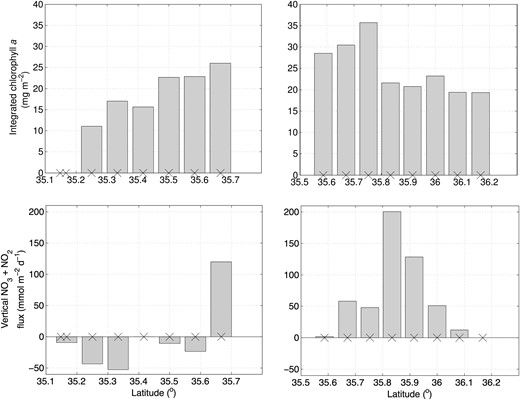
Vertical nitrate flux at 60 m depth (mmol m−2 day−1) (top panel) and chlorophyll a integrated over the top 60 m (mg m−2). The locations of the stations are shown as crosses along the x-axis.
Depth-integrated chlorophyll a in the upper 60 m (Fig. 3, top panels) was highest at 35.75°N (35.7 mg m−2), whereas the southernmost station along transect E had the lowest value (7.8 mg m−2). Integrated chlorophyll a values were generally highest at the front and drop off to the north and the south. However, the station with the high depth-integrated chlorophyll a did not coincide with the highest value of w(NO2 + NO3), and stations along transect E with negative values of w(NO2 + NO3) just south of the front have depth-integrated chlorophyll a values comparable with those north of the front along transect D where w(NO2 + NO3) is positive.
Photosynthetic and photoprotective pigments
We observed vertical and horizontal variations in the ratios of the PPC and photosynthetic carotenoids (PSC) to total chlorophyll a (TChla) (Fig. 4). Stations closest to the front showed little vertical variation in PPC:TChla. In contrast, there were lower values of PSC:TChla at the surface. To the north of the front, along transect D, both ratios exhibited more marked vertical variation, especially between 35.8°N and 36°N. High values of PPC:TChla (up to 0.3) and very low values of PSC:TChla were associated with a lens of fresher Oyashio water at the surface. South of the front along transect E, the vertical structure was less pronounced than on transect D. South of 35.55°N, there was an increase in PPC:TChla in the upper 20 m, with lower values below. An increase in the ratio at 80 m may not be significant, since TChla was at very low concentrations there.
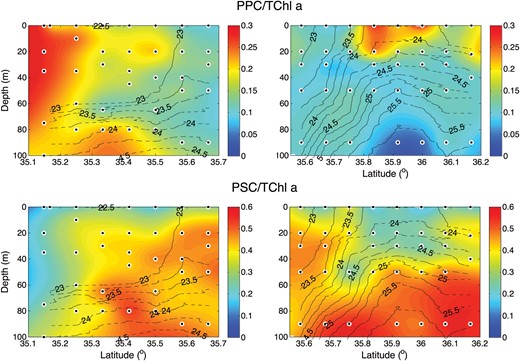
Ratio of photoprotective pigments to chlorophyll a (PPC:TChl a) (top panels), and the ratio of photosynthetic pigments to chlorophyll a (PSC:TChl a) (bottom panels) for transect D (left) and transect E (right). Solid black lines define σt contours.
Phytoplankton community structure
Picophytoplankton
Picophytoplankton (<2 μm) were identified and enumerated by flow cytometry, revealing a significant spatial variability in picophytoplankton abundances, both vertically and across the front (Fig. 5). Prochlorococcus and Synechococcus were most abundant to the south of the front. Prochlorococcus dominated picoplankton abundance at the extreme southern end of the transects, with a progression to higher Synechococcus abundances closer to the core of the front. In section D, Synechococcus was abundant on both sides of the front, with maxima on either side of the 23.75 kg m−3 σt surface, in the top 40 m of the water column. This area of high Synechococcus abundance to the north of the front is located just above the domed nutricline where concentrations of nitrate and phosphate were elevated. Picoeukaryotes are also most abundant to the south of the front, although their maximum appeared to coincide with the core of the front in section D, in contrast to the offset of Synechococcus. Distributions of divinyl chlorophyll a (DVChla), a marker pigment for Prochlorococcus, and Zeaxanthin (Zea), a marker pigment for cyanobacteria (Fig. 7) correspond well to the distributions of Prochlorococcus and Synechococcus observed by flow cytometry.
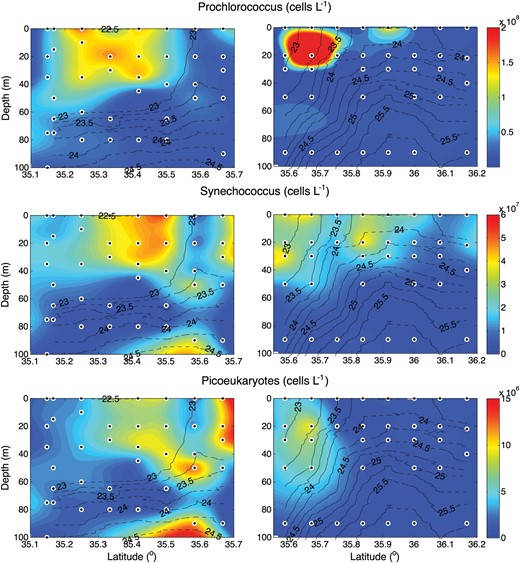
Sections of the abundance of, from top to bottom, Prochlorococcus, Synechococcus and picoeukaryotes all in units of cells L−1. Solid black lines define σt contours.
Nano- and microphytoplankton
More than 50 species of nano- (2–20 μm) and microphytoplankton (>20 μm) were identified and enumerated by light microscopy. Here, we present their distributions organized by major group: diatoms, dinoflagellates and haptophytes (Fig. 6). We also show the distribution of the pigments Fucoxanthin (Fuco), Peridinin (Peri) and 19′-hexanoyloxyfucoxanthin (Hex Fuco), which are marker pigments for diatoms, autotrophic dinoflagellates and haptophytes, respectively (Fig. 7). They are found predominantly at and to the north of the core of the front. Diatoms and dinoflagellates have notably patchier distributions than the picoplankton and haptopytes. Haptophytes are the most closely associated with the front itself, with an abundance maximum of ∼45 600 cells L−1 at 35.7°N along transect D where isopycnals are steepest. Diatoms are most closely associated with nutrient gradients at the nutricline and along the nutrient ‘tongue’ (transect E), but are also present in patches near the surface. Dinoflagellates are mostly found close to the surface, with the exception of a patch at 80 m near the nutrient tongue (transect E). The marker pigment distributions are broadly consistent with the cell counts, although we do see some marked differences, particularly between diatom and Fuco distributions. These differences are most likely to be due to variations in the cell concentration of pigments, which is controlled by physiological responses to environmental conditions (e.g. light, nutrient status).
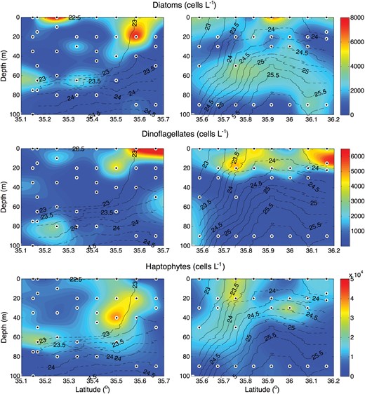
Sections of the abundance of, from top to bottom, diatoms, dinoflagellates and haptophytes all in units of cells L−1. Solid black lines define σt contours.
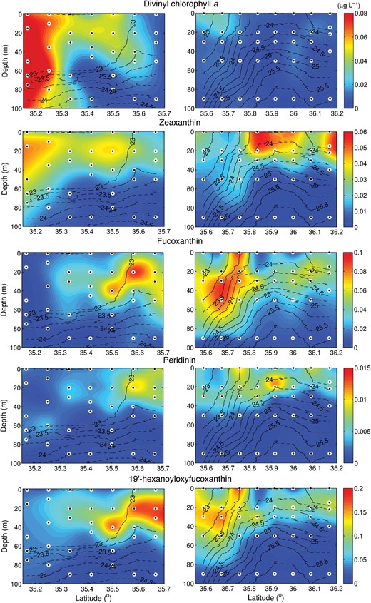
Sections of the abundance of, from top to bottom, divinyl chlorophyll a, zeaxanthin, fucoxanthin, peridinin and 19′-hexanoyloxyfucoxanthin, all in units of μg L−1. Solid black lines define σt contours.
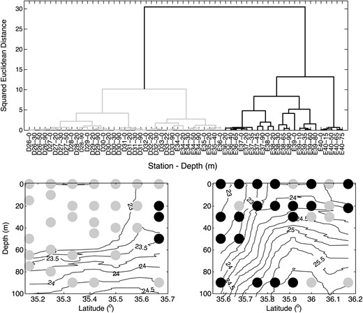
Top panel: dendrogram showing the phytoplankton community structure in the study area, using combined data from both transects D and E. Each data point is identified on the x-axis by its station number and depth. The bottom panel shows the location of the two phytoplankton community groups mapped back into space across the front, σt contours are shown by solid black lines.
DISCUSSION
Relating biogeography to physical features
A general observation, based on the microscopy, pigment and flow cytometric data, is that the abundance maxima of phytoplankton functional types are not co-located. The complex and fine-scale structures exhibited by the organisms suggest a strong role for the transport and interleaving of ‘biomes’ dominated by specific organism types, both by along-front and cross-frontal motions. This is consistent with the view of D'Ovidio et al. (D'Ovidio et al., 2010) in an analysis of plankton populations on the Patagonia shelf observed by remote sensing.
Following Yamamoto et al. (Yamamoto et al., 1988), we used the dissimilarity of the squared Euclidean distance between data points to cluster the phytoplankton communities found at each station into distinct assemblages (Fig. 8, prepared using the Ward method). We perform the analysis using the picophytoplankton flow cytometry and microphytoplankton cell counts, all of the data are normalized prior to performing the clustering. The phytoplankton assemblages fall into two distinct groups, largely separated by the front and corresponding to subtropical and subpolar communities. The presence of waters with ‘subtropical’ characteristics to the north of the front reflect the warm filament (Fig. 1B), left behind following a northward excursion of the Kuroshio, along with its subtropical phytoplankton assemblage. Ultimately, the filament will be eroded by small-scale mixing and result in a net transfer of properties from the stream into subpolar waters contributing to the large-scale dispersal and mixing of populations and the maintenance of local diversity in the plankton population (Clayton et al., 2013).
Similar analyses of the Kuroshio Front (Yamamoto et al., 1988) and California Current (Taylor et al., 2012) both identified a third assemblage specifically associated with the front. This may be attributable to along-front advection of upstream communities, e.g. (Cavender-Bares et al., 2001), or a local response to frontal-scale vertical circulations. The analysis here did not reveal such a biome in this data set, possibly because of the lower spatial resolution in horizontal sampling (9 vs. <3 km).
How does the frontal circulation affect the light and nutrient environment?
A significant feature of the data set is the strong variation in chlorophyll, nutrient concentrations and community composition on short spatial scales, both across the front and with depth. These are, at least in part, due to the vigorous frontal-scale vertical velocities and shear associated with the swift Kuroshio current, which act on timescales close to, and even shorter than, cell division and acclimation. The concurrent physical survey of the study region (Nagai et al., 2012) showed that the observed region of the front was subject to strong mixing and vertical circulations of ∼ O (10 m day−1) or more. The impact of these frontal scale circulations was evident in the pigment distributions, which were not acclimated to the local light environment in some profiles, as well as unusual features including the vertical inversions in the nutrient profiles. To the north of the front in stable, stratified waters (see Transect D) the ratio of photoprotective/photosynthetic pigments to chlorophyll (PPC:TChla/PSC:TChla) decreased/increased with depth following the light gradient, as is typically the case. In contrast, in the vicinity of the front, both pigment ratios were relatively uniform with depth, suggesting that phytoplankton in the frontal zone were transported vertically in the water column more rapidly than acclimation to ambient light conditions.
Strong vertical velocities at the front were responsible for a localized increase in the vertical flux of nutrients to the surface. We found that mesoscale and submesoscale dynamics interacted to modulate the supply of nutrients to the surface layer. Mesoscale dynamics drove the doming up of the nutricline to the north of the front, most pronounced along transect D but also apparent at the northernmost station of transect E. Elevated turbulent mixing, driven by the ageostrophic frontal circulation, and measured directly by microstructure in the surface mixed layer along transect E (Nagai et al., 2012) also acted to inject nutrient-rich water into the surface layer.
One of the more unusual features observed in the nutrient distributions was the inversion in the vertical distributions of nutrients associated with the base of the mixed layer along transect E, flanked above and below by lower concentrations. Similar features are apparent in published sections from the Kuroshio (Yamamoto et al., 1988; Ishizaka et al., 1994), and across the East Australian Current (Baird et al., 2008), although the respective authors did not comment on them. Here, we consider two candidate explanations for such a feature. First, during the cruise, the averaged wind was aligned down-front, in the same direction as the frontal jet on the south side of the Kuroshio (Nagai et al., 2012). A down-front wind can result in the transport of denser waters from the northern side of the front over the lighter waters on the southern side of the front by Ekman transport. This induces a mechanical convection (Thomas and Lee, 2005) which generates elevated turbulence (D'Asaro et al., 2011; Nagai et al., 2012) resulting in the subduction of well mixed water along isopycnals, possibly causing a ‘tongue’ of nutrient rich waters as observed. An alternative mechanism is the action of near-inertial internal waves which, with a sufficiently large amplitude, are subject to Stoke's drift (Thomas and Lee, 2005), driving a net southward transport of high nutrient waters. Nagai et al. (Nagai et al., 2012) showed that there was a stronger downward energy propagation of internal waves in transect E, coincident with the location of the nutrient ‘tongue’, indicating that near-inertial waves are playing a role in the generation of this feature. We also observed patches of high abundances of diatoms, dinoflagellates and haptophytes all associated with the same or nearby data points as the nutrient tongue. The cluster analysis identifies these points as belonging to a subtropical assemblage, so it is likely that the elevated nutrient supply is fuelling the growth of larger phytoplankton cells, although it may also be possible that some of these larger species are the residue of a subpolar population that was transported with the nutrient rich waters, originating north of the front. Similarly, the nutrient distributions observed along transect D were very patchy, especially in the upper 40 m of the northern half of the transect, with several isolated patches of higher nutrient water. Although we do not have direct measurements of the turbulent mixing along transect D, we do for transect B, which was also offset to the north of the front and can be thought of as being upstream of transect D. Along transect B, turbulent subsurface mixing was very strong (Nagai et al., 2012), which, we hypothesize, coupled with the mesoscale uplifting of the nutricline, resulted in the entrainment of high nutrient water from the nutricline into the surface mixed layer.
We did not find a clear relationship between the vertical nutrient flux, chlorophyll a standing stock and the mixed layer depth, indicating that cross-frontal processes are important in generating the observed distribution of phytoplankton biomass. The maximum chlorophyll a concentration was two-fold higher at the front (transect D) than at stations either side of it, but there was a clear spatial offset between the maximum chlorophyll a concentration and the maximum vertical nitrate flux. This offset between the maximal vertical nutrient fluxes and the maximal depth-integrated chlorophyll suggests that nutrients were transported laterally before they could be taken up by phytoplankton in situ. In other words, the timescale for physical transport was shorter than biological uptake by the population: the highest vertical velocity estimated for our study area was ∼ 30 m day−1 just north of the front [although this is likely to be an underestimate, Allen et al. (Allen et al., 2001)]. This yields a residence time with respect to vertical motion of ∼0.6–2 days for the range of observed mixed layer depths (20–60 m, Figure 1C and D), which is comparable to the characteristic timescale for phytoplankton growth (and specific affinity) under resource replete conditions, but shorter than the 3-day lag between nutrient supply and production described in the Kuroshio by Yamazaki et al. (Yamazaki et al., 2009). Similarly, elevated values of depth-integrated chlorophyll along transect E, where the vertical nitrate flux was negative at all but the northernmost station, must have been the result of the lateral advection of either chlorophyll- or nutrient-rich waters away from their source.
CONCLUSIONS
In summary, the taxonomic composition of the phytoplankton communities near the front fell into two broad groups associated with the subtropical and subpolar biomes, which are brought into close proximity at the front. While fast fine-scale physical processes lead to interleaving and modification of the communities, we did not see a ‘special’ community associated with frontal conditions in this data set. There was evidence of a remnant of subtopical waters, with associated populations, left behind to the north of the current following a meridional excursion of the Kuroshio. This feature would ultimately have been eroded by local mixing processes, and such phenomena may contribute significantly to the exchange of populations and genetic material across the front, enhancing the local diversity of the phytoplankton population (Clayton et al., 2013). The strong physical forcing and instabilities at the front drive small-scale physical motions that perturb the biological system more rapidly than either acclimation or resource uptake can respond. This leads to the appearance of un-acclimated populations and even nutrient inversions in the environment of the front.
While revealing, this data set is still relatively sparse and reveals just a snapshot of a complex and continually evolving system. Looking forward, to fully understand the bio-physical dynamics in such regions will require alternative sampling methods, for example appropriately equipped AUVs, which can capture the fine spatial scales and fast timescales on which frontal processes are acting. In addition, high-resolution (idealized) simulations can be a tool for testing hypothesized mechanisms and quantifying the integrated impact of these fine-scale physical biological interactions.
FUNDING
This work was supported by the Gordon and Betty Moore Foundation Microbiology Initiative, the National Science Foundation, National Aeronautics and Space Administration (NNX13AC34G to M.F. and S.C.), and the Japan Society for the Promotion of Science (Kakenhi 24684036 to T.N.).
ACKNOWLEDGEMENTS
The authors would like to thank Prof. Hidekatsu Yamazaki, Dr Mark Doubell and the Captain and crew of the R/V Natsushima for their assistance with logistics leading up to and during the cruise. We would also like to thank Prof. Sallie Chisholm and Prof. Edward DeLong at MIT for providing support for flow cytometry and sample storage.
REFERENCES
Author notes
Corresponding editor: Roger Harris
