


Abstract
The ability of pelagic copepods to remotely detect and encounter potential sexual partners is a critical issue in zooplankton ecology. In calanoid copepods, mate-finding behaviour involves either chemical or hydromechanical cues. Here, I first provide a detailed description of the three-dimensional swimming behaviour of Eurytemora affinis, males, non-ovigerous females and ovigerous females swimming freely in the absence of chemical and hydromechanical cues and discuss potential reasons for the discrepancies observed in the literature. I further demonstrate that E. affinis males modify their swimming behaviour in response to a diffuse background of pheromone concentrations, which can be thought of as an adaptation to increase the encounter rate and follow trail mimics containing female scent. I finally describe the mate-seeking behaviour of E. affinis and show how males swimming freely in a three-dimensional environment modify their direction of motion upon encountering the pheromone trails of females and subsequently follow female trails over distance and duration of nearly 15 cm and 36 s until they hydromechanically sense the female and lunge at her. The relevance of these results is discussed in the general framework of search pattern strategies and the relative contribution of chemical versus hydromechanical cues in relation to the turbulent nature of the surface ocean.
INTRODUCTION
The calanoid copepod Eurytemoraaffinis (Poppe, 1880) typically dominates the zooplankton community in the oligomesohaline zone of most estuaries of the North Hemisphere, where it is considered as a key species (Lee, 2000; Mouny and Dauvin, 2002; Devreker et al., 2008). A considerable amount of work has hence been devoted to E. affinis distribution and abundance (Roddie et al., 1984; Hough and Naylor, 1992; Andersen and Nielsen, 1997; Morgan et al., 1997; Kimmerer et al., 1998; Gasparini et al., 1999; Devreker et al., 2009), physiology (Roddie et al., 1984; Kimmel and Bradley, 2001), life cycle, post-embryonic development and reproduction (Ban, 1994; Andersen and Nielsen, 1997; Koski et al., 1999; Devreker et al., 2004, 2007, 2009) and phylogeography (Lee, 2000; Lee et al., 2003, 2007; Winkler et al., 2011). However, information on E. affinis swimming behaviour is still scarce and contradictory (Seuront, 2006, 2010a, b, 2012; Michalec et al., 2010; Souissi et al., 2010) and information on their mating behaviour limited to the early work of Katona (Katona, 1973) who showed that males were able to locate stationary females located up to 20 mm away and suggested the role of female pheromones in male mate-finding behaviour.
Several types of mate-finding behaviour involving either chemoreception or mechanoreception have been observed in marine copepods to increase the probability of mate encounter in environments where planktonic copepod are often located 10's to 100's of body lengths away in a three-dimensional environment. For instance, Temora longicornis females have been shown to react to chemical exudates of conspecific males with little hops, hence increasing encounter probability with potential mates (van Duren et al., 1998). Active mate-searching behaviour is, however, essentially exhibited by males. Typically, males search for chemical cues signalling the presence and the position of the females. In some species, such as Calanus marshallae (Tsuda and Miller, 1998), Centropages hamatus (Goetze, 2008), Centropages typicus (Bagøien and Kiørboe, 2005a, b; Goetze, 2008), T. longicornis (Doall et al., 1998; Weissburg et al., 1998; Yen et al., 1998, 2004; Goetze and Kiørboe, 2008; Seuront, 2011a), Temora stylifera (Goetze and Kiørboe, 2008) and Hesperodiaptomus shoshone (Yen et al., 2011) females leave a chemical trail in their wake, which males may detect and follow. Pheromones are also involved in the form of pheromone clouds in the freshwater copepod Leptodiaptomus ashlandi (Nihongi et al., 2004) and in the marine species Pseudocalanus elongatus (Kiørboe et al., 2005) and Oithona davisae (Kiørboe, 2007). Some freshwater (Cyclops scutifer; Strickler, 1998) and marine copepods (Acartia tonsa; Doall et al., 2001; Bagøien and Kiørboe 2005a, b) also increase their perceptual distance beyond physical contact via hydromechanical cues to detect and pursue females. In contrast to hydromechanical signals that rapidly decay (Yen et al., 1998), pheromone trails can be followed over many body lengths, and trail following can occur over distances up to ca. 200 mm (Bagøien and Kiørboe, 2005a, b). It is hence likely to be the most effective mate-finding behaviour, hence leading to improved encounter rates between potential mates, especially at low population density (Kiørboe et al., 2005).
Chemosensory abilities may be particularly critical for E. affinis males to locate and track conspecific females as estuarine waters may be contaminated by a range of organic and inorganic pollutants (Louchouarn and Lucotte, 1998; Matthiessen and Law, 2002; Soares et al., 2008). These pollutants are likely to influence the perceptive abilities, hence the swimming behaviour of zooplankton (Faimali et al., 2006; Garaventa et al., 2010; Cailleaud et al., 2011). This has recently been shown from the escape reactions of T. longicornis and E. affinis in response to patches contaminated at 0.01, 0.1 and 1% with the soluble fraction of diesel oil (Seuront, 2010a, 2012). In this context, I first provide a detailed description of the swimming behaviour of E. affinis, i.e. males, non-ovigerous females and ovigerous females swimming freely in the absence of chemical and hydromechanical cues. The chemosensory abilities of E. affinis males are assessed through their behavioural response to (i) estuarine water conditioned with non-ovigerous females and ovigerous females and (ii) chemical trail mimics created by non-ovigerous and ovigerous females. I finally describe the mate-seeking behaviour of E. affinis and show that males use both chemoreception and mechanoreception to detect and capture remote and close females, respectively.
METHOD
Eurytemora affinis collection and acclimation
Eurytemora affinis individuals were collected from the Seine estuary using a WP2 net (200-µm mesh size) at a temperature of 15°C and a salinity of 4 at low tide near the “Pont de Tancarville” (49°28′26"N, 0°27′47"W), where previous studies have observed maximum abundance (e.g. Mouny and Dauvin, 2002). Specimens were gently diluted in 30-L isotherm tanks using in situ estuarine water and transported to the laboratory where adult males, non-ovigerous females and ovigerous females were immediately sorted by pipette under a dissecting microscope. Animals were then kept separately in aerated 20-L aquaria filled with filtered (Whatman GF/C glass–fibre filters, porosity 0.45 µm) and autoclaved estuarine water for 24 h at a temperature of 16°C and a salinity of 4 before experimentation.
Behavioural observations
Cue-free swimming behaviour
To assess the innate properties of the swimming behaviour of E. affinis, adult males, non-ovigerous females and ovigerous females were exposed to cue-free estuarine water in the absence of conspecific. Cue-free estuarine water was prepared from in situ estuarine water filtered (Whatman GF/C glass–fibre filters, porosity 0.45 µm) and subsequently autoclaved. Cue-free estuarine water was transferred in sterile plastic vials and frozen until the behavioural experiments took place (Yen et al., 2011). All subsequent experiments were conducted on 10 individuals (males, non-ovigerous females and ovigerous females). Individuals were only used once, each experiment was replicated five times, and the experiments were randomized.
Behavioural response to trail mimics
To assess if E. affinis follow a chemical trail in the absence of conspecifics, males were exposed to chemical trail mimics created by male- and female-conditioned estuarine water. I followed a procedure modified from the very elegant approach designed by Yen et al. (Yen et al., 2004, 2011) who doubly labelled female-conditioned water with high-molecular-weight dextran to increase the difference in the refractive index. This enables the creation of trail mimics that would be visible using Schlieren optics to determine if the marine and freshwater copepods T. longicornis and H. shoshone would follow a chemical trail in the absence of females. To create male- and female-conditioned water, non-ovigerous and ovigerous females were placed separately in beakers containing control filtered and autoclaved estuarine water, at a density of 10 animals/L. Males, non-ovigerous females and ovigerous females were allowed to condition the water for 24 h. After incubation was completed, conditioned water was transferred to sterile plastic vials and frozen until the behavioural experiments took place (Yen et al., 2011). Trail mimics were subsequently created by feeding dense estuarine water, i.e. a mixture of estuarine water and high-molecular-weight dextran (MW of 500 000 at 5 10−3 g mL−1; Yen et al., 2004), either scent-free or preconditioned with males, non-ovigerous females and females tagged with fluorescein into the behavioural container (a 3.375-L cubic glass chamber, i.e. 15 cm × 15 cm × 15 cm) by an electronic syringe pump via capillary tubes at a very slow rate (ca. 0.02 mL min−1), resulting in a trail speed of 0.05 mm s−1. The flow generated is nearly 50- and 10-fold slower than the swimming speed of E. affinis non-ovigerous (2.46 ± 0.18 mm s−1) and ovigerous females (0.66 ± 0.06 mm s−1; Seuront, 2006, 2012), hence expected to minimize the related hydromechanical disturbance. Control trails contained (i) filtered and autoclaved estuarine water and (ii) filtered and autoclaved male-conditioned estuarine water. Treatment trails contained (i) filtered and autoclaved estuarine water conditioned with non-ovigerous females and (ii) filtered and autoclaved estuarine water conditioned with ovigerous females. For each trail-mimic condition, 10 males were introduced in the experimental container once the trails were fully developed and reached the bottom of the container (i.e. 50 min). Each trail-mimic experiment lasted for 1 h and was replicated five times. The behavioural container, syringes and capillary tubes were rinsed with acetone and distilled water and allowed to dry between trials to remove any chemical scent.
Mate-seeking behaviour
To assess if E. affinis males would change their swimming behaviour in response to male or female scent, males were first exposed to male- and female-conditioned estuarine water. Male- and female-conditioned water was prepared and stored as described above. Subsequent behavioural experiments were conducted on 10 males. Individuals were only used once, each behavioural experiment was replicated five times and the experiments conducted on males, non-ovigerous females and ovigerous females were randomized.
To ensure that trail-following behaviour was performed by males towards females and that no male–male or female–female trail following occurred, control experiments were run using 5 males × 5 males and 5 non-ovigerous females × 5 non-ovigerous females, 5 ovigerous females × 5 ovigerous females and 5 non-ovigerous females × 5 ovigerous females. No evidence of mate-seeking behaviour was ever found towards the conspecific of the same sex. Eurytemora affinis mate-seeking behaviour was subsequently assessed through the swimming behaviour of adult males in the presence of either non-ovigerous females or ovigerous females. Mate-seeking behavioural experiments (i.e. 5 males × 5 non-ovigerous females and 5 males × 5 ovigerous females) were replicated 10 times and randomized. As the sex of the copepods was not obvious from video recordings for experiments run with males and non-ovigerous females, when a pair remained together after contact, the pursuer was assumed to be a male and the pursued a female (Yen et al., 2011). The prosome length of E. affinis males (0.96 ± 0.01 mm;  ), non-ovigerous females (1.09 ± 0.01 mm) and ovigerous females (1.11 ± 0.02 mm) used in the experiments did not significantly differ between treatments and replicates (Kruskal–Wallis test, P > 0.05).
Video set-up and behavioural experiments
Prior to each experiment, experimental individuals were transferred in the experimental filming set-up (a 15 cm × 15 cm × 15 cm glass chamber) filled up with uncontaminated seawater and the corresponding treatments and were allowed to acclimatize for 15 min (Seuront, 2006). All experimental individuals were used only once, and no narcosis (lack of motility) was ever observed in any of the tested individuals. The experimental chamber was rinsed with acetone and distilled water and allowed to dry between trials to remove any chemical scent.
The three-dimensional swimming and mate-seeking behaviours of E. affinis were observed at a rate of 25 frames s−1 using two orthogonally oriented and synchronized infra-red digital cameras (DV Sony DCR-PC120E) facing the experimental chamber. Six arrays of 72 infra-red-light-emitting diodes connected to a 12-V DC power supply, provided the only light source from the bottom of the chamber. The cameras overlooked the experimental chamber from the side, and the various components of the set-up were adjusted so that the copepods were adequately resolved and in focus. Specifically, to ensure that the field of view was geometrically uniform over the volume of observation, a reference grid (i.e. a 3 mm thick 15 cm × 15 cm transparent PVC sheet, with 196 evenly spaced circular dots of 1 mm in diameter) was placed vertically every centimetre in the experimental container, and the camera parameters were subsequently chosen as those minimizing the projection error between the location of observed and predicted points. This technique, known as bundle adjustment (Triggs et al., 1999; Hartley and Zisserman, 2004), is classically used as the last step of feature-based structure and motion estimate computer vision algorithms to obtain optimal estimates (see, for example, Lourakis and Argyros, 2009). The projection error has been minimized using the non-linear least-squares Levenberg–Marquardt algorithm used elsewhere as an optimization procedure to fit the simplified canonical law to empirical data (Seuront, 2013). Besides, the resolution of the set-up (ca. 100 μm) allows the unambiguous assessment of the orientation of the rostro-caudal body axis.
Each experiment lasted 60 min, after which valid video clips were selected for analysis. Valid video clips consisted of pathways in which the animals were swimming freely, at least two body lengths away from any chamber walls or the surface of the water (Seuront, 2006). All the experiments were conducted at a temperature of 16°C and a salinity of 6 in the dark and at night (consistently between 10 p.m. and 2 a.m., as preliminary experiments did not show any significant change in E. affinis behaviour over this temporal window; Seuront, unpublished data) to avoid any potential behavioural artefact related to the diel cycle of the copepods (Seuront, 2011b). Selected video clips were captured (DVgate Plus) as MPEG movies and converted into QuickTime TM movies (QuickTime Pro), after which the x, y and z coordinates of swimming pathways were automatically extracted and subsequently combined into a 3D picture using LabTrack software (DiMedia, Kvistgård, Denmark). The time step was always 0.04 s, and output sequences of (x, y, z) coordinates were subsequently used to characterize the motion behaviour. Note that to work on statistically consistent swimming paths, paths of similar durations (55–65 s) were considered for the behavioural analyses (Seuront, 2006).
Behavioural analysis
Swimming behaviours
Three kinds of swimming behaviours were considered for males, non-ovigerous females and ovigerous females: (i) cruising, in which their rostro-caudal body axes were aligned with the direction of motion, whether they were swimming up, down or horizontally, (ii) hovering, in which copepods typically travel upwards at slow speed in relatively linear directions with the rostro-caudal body axis oriented upwards and with frequent horizontal reorientation hops (Doall et al., 1998), (iii) breaking [referred to as “hovering” in Seuront (Seuront, 2006)], in which they remain motionless, with their rostro-caudal axes oriented upwards, and (iv) passive sinking, i.e. downward vertical motion, with tail down. Each behavioural activity was quantified in terms of time allocation percentage for each category of organisms.
Swimming speed

Swimming path complexity
The complexity of swimming paths during non-mating and mating sequences was assessed using fractal analysis. In contrast to standard behavioural metrics such as turning angle and net-to-gross displacement ratio, fractal analysis and the related fractal dimension DF have the desirable properties to be independent of the measurement scale and to be very sensitive to subtle behavioural changes that may be undetectable in other behavioural variables (Coughlin et al., 1992; Seuront and Leterme, 2007; Seuront and Vincent, 2008; Seuront, 2011a, b, 2012). Fractal analysis has been applied to describe the complexity of zooplankton and ichthyoplankton swimming paths (Coughlin et al., 1992; Bundy et al., 1993; Dowling et al., 2000; Seuront et al., 2004a, b, c, d, 2006, 2010c, 2011a, b; Uttieri et al., 2005, 2007a, 2008; Seuront and Vincent, 2008; Ziarek et al., 2011; Michalec et al., 2012). The fractal dimensions of E. affinis swimming paths were estimated using two different, but conceptually similar, methods to ensure the reliability of fractal dimension estimates; see, for example, Hastings and Sugihara (Hastings and Sugihara, 1993) and Seuront (Seuront, 2010c) for reviews.

 sampling windows as NO(δ). The mass m(δ) of occupied pixels is then defined as:

 and
and  used to characterize the complexity of a swimming path. In contrast to Michalec et al. (Michalec et al., 2012), I did not use a correction term in the determination of the fractal dimensions Db and Dm as none of the scripts used to implement Equations (1)–(3) returned fractal dimensions that were statistically significantly different (P > 0.05) from (i) a dimension of 1 and 2 when respectively run on vectors of random length and orientation or surfaces of random surface and orientation and (ii) the expected fractal dimensions of theoretical fractal objects; here, I used the well-known Koch snowflake (D = 1.262), the Koch island (D = 1.5), the Sierpinskin carpet (D = 1.893) and the Sierpinski gasket [D = 1.585; see, for example, Hastings and Sugihara (Hastings and Sugihara, 1993) and Seuront (Seuront, 2010c) for further details on those objects].
The appropriate range of scales l [Equation (1)] and δ [Equation (3)] to include in the regression analyses was chosen following the R2–SSR criterion (Seuront et al., 2004a; Seuront, 2010c). Briefly, I consider a regression window of varying width ranging from a minimum of five data points (the least number of data points to ensure the statistical relevance of a regression analysis) to the entire data set. The windows are slid along the entire data set at the smallest available increments, with the whole procedure iterated n − 4 times, where n is the total number of available data points. Within each window and for each width, I estimated the coefficient of determination (r2) and the sum of the squared residuals for the regression. I subsequently used the values of l [Equation (1)] and δ [Equation (3)], which maximized the coefficient of determination and minimized the total sum of the squared residuals to define the scaling range and to estimate the related dimensions Db and Dm. Note that Db and Dm are bounded between 1 for a linear swimming path and 2 for a path so complex that it fills the whole space available.
Mate-seeking behaviour
Behavioural sequences were classified as non-mating and mating events. Non-mating events correspond to behavioural sequences observed before the initiation of mate pursuit. Mating events were subcategorized as chemically and hydromechanically mediated mating events. Specifically, chemically mediated mating events were related to the ability of males to detect female pheromone trails and to travel towards the female following her pheromone trail and classified as tracking, contact and capture events. In unsuccessful tracking events, the male detects the pheromone trail and initiates a tracking behaviour (i.e. defined by initiation of “spinning” behaviour, in which the male's position oscillated and he appeared to be rotating around the longitudinal body axis; Doall et al., 1998), travels directly towards the female following the pheromone trail, but loses the trail prior to contact with the female. In contact events, the male follows the pheromone trail to the point of mate contact, but fails to capture the female; and in capture events, the male successfully tracks a potential mate and captures her. In contrast, in hydromechanically mediated mating events, males directly lunge at females independently of their pheromone trails, when they travel in proximity of the females.
Chemically and hydromechanically mediated perceptive distances
The perceptive abilities of males were assessed using three chemically mediated perceptive distances  ,
,  and
and  and two hydromechanically mediated perceptive distances
  and
and  (Fig. 1). The chemically mediated perceptive distance
  is the direct linear distance between the male's and the female's trail when the male initiates a tracking behaviour;
  is the direct linear distance between the male and the female at the initiation of mate pursuit behaviour (Yen et al., 2011) and
  the male distance from female track-line during tracking. The hydromechanically mediated perceptive distance
  was calculated as the linear distance between the male and the female when the male lunges to catch the female after successfully following her pheromone trail (Yen et al., 2011). The hydromechanically mediated perceptive distance
  corresponds to the distance at which a male directly lunges at females independently of their pheromone trails.
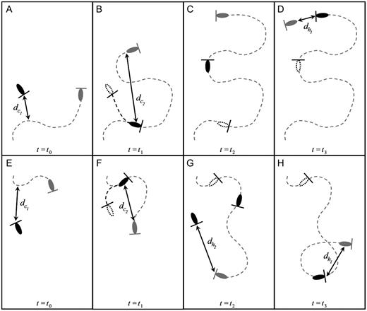
Illustration of the chemically mediated perceptive distances  and
and  and the hydromechanically mediated perceptive distances
  and
and  using two distinct schematical temporal sequences (A–D and E–H). The chemically mediated perceptive distance
  is estimated as the direct distance between the male and the female's trail when the male initiates a tracking behaviour (A and E), wheras
  is the direct linear distance between a male (black) and a female (grey) at the initiation of mate pursuit behaviour (B and F). The hydromechanically mediated perceptive distance
  is the linear distance between the male and the female when the male lunges to catch the female after successfully following her pheromone trail (D and H). The hydromechanically mediated perceptive distance
  is the distance at which a male directly lunges at females independently of their pheromone trails (G).
Mate-seeking behaviour accuracy and efficiency
The accuracy with which males followed female trails was estimated using the male-to-female displacement ratio,  , where
  is the length of the male tracking trajectory and
  the length of the female trajectory (Doall et al., 1998); MFDR = 1 when the male's trajectory exactly matches the female's one, MFDR < 1 characterized males taking short-cuts along female's trajectories, and MFDR > 1 characterized males swimming with more frequent turns than females.
The efficiency of males to detect female pheromone trail was quantified by the distance  (see above), and the age of the female's trail upon detection by the male. The age of the trail at the time of detection was calculated as the difference between the time when the female was positioned at the detection point to the time when the male initiated pursuit from this point. The tracking time was further estimated as the time elapsed between the male initiation of pursuit and the attempted capture of the female.
Finally, the contact and capture efficiencies were estimated as the contact and capture rates defined by the number of contact and capture events normalized by the number of tracking events.
Statistical analyses
Because the behavioural parameters were non-normally distributed (Kolmogorov–Smirnov test, P < 0.01), non-parametric statistics were used throughout this work. Pairwise comparisons were carried out using the Wilcoxon–Mann–Whitney U-test (WMW test hereafter). Multiple comparisons between males and females were conducted using the Kruskal–Wallis test, and the Jonckheere test for ordered alternatives (Siegel and Castellan, 1988) was used to identify distinct groups of fractal dimensions.
RESULTS
Eurytemora affinis swimming behaviour in cue-free estuarine water
A total of 55, 47 and 45 swimming paths were, respectively, observed for E. affinis males, non-ovigerous females and ovigerous females.
Males and non-ovigerous females exhibited relatively comparable curvilinear swimming paths developed similarly in the vertical and horizontal planes (Fig. 2a and b). In contrast, ovigerous females exhibited rectilinear trajectories mainly restricted to the vertical plane and characterized by an alternation between hovering and sinking bouts (Fig. 2c). The time allocated to distinct behaviours (Fig. 3a) and swimming speed (Fig. 4a) also differs between sexes; in particular, ovigerous females are behaviourally very distinct from both males and non-ovigerous females.
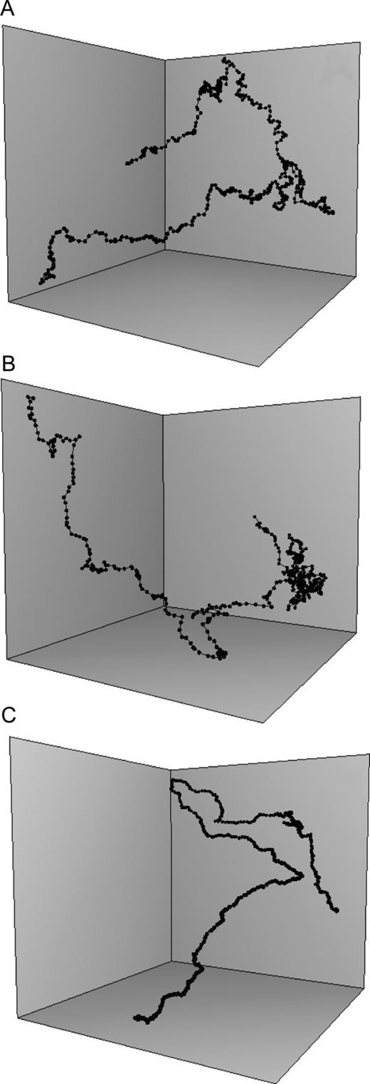
Representative three-dimensional trajectories of E. affinis males (A), non-ovigerous females (B) and ovigerous females (C). Each trajectory has been plotted in a standardized volume of 15 cm × 15 cm × 15 cm.
![Fraction of time allocated by E. affinis males (M), non-ovigerous females (NOF) and ovigerous females (OF) to cruising (black), hovering (dark grey), sinking (light grey) and breaking (white) in GF/C filtered and autoclaved estuarine water (top) and by E. affinis males swimming freely in GF/C filtered and autoclaved estuarine water conditioned with males [M(M)], non-ovigerous females [M(NOF)] and ovigerous females [M(OF)] (bottom). Error bars are standard deviations.](https://oup.silverchair-cdn.com/oup/backfile/Content_public/Journal/plankt/35/4/10.1093/plankt/fbt039/2/m_fbt03903.jpeg?Expires=1716462184&Signature=G7aCvQTZt-y-dg1iUYSzN8v~qgpBNSnUs6TQzlf2l~bvAvWZIftqKlVqfjIU4Vy1lFwm02FhtOFN06vMzDCfFihLC7cKfSXLjJh3UACkPFbpA5os9XFO3GqcYq~lyDAy89fOD6hKjOqUI5dSHdcEyZjiYrraXnZcuAUkKnEURGaps6Q5pnTSX4l1cFgSD97RV3pqPcNsKgh3bhiy9MofrE85htILBR52HIVd3rg79oarabQlxIiHG-zCYRCxO8V1OpqUXjD9LrV-e4B9fcYmSZjNtA367IQsW99brykhpBj40hVfaaf~9FFg9CdjiPFLyvm7LAIag8UZgLjolM760A__&Key-Pair-Id=APKAIE5G5CRDK6RD3PGA)
Fraction of time allocated by E. affinis males (M), non-ovigerous females (NOF) and ovigerous females (OF) to cruising (black), hovering (dark grey), sinking (light grey) and breaking (white) in GF/C filtered and autoclaved estuarine water (top) and by E. affinis males swimming freely in GF/C filtered and autoclaved estuarine water conditioned with males [M(M)], non-ovigerous females [M(NOF)] and ovigerous females [M(OF)] (bottom). Error bars are standard deviations.
![(Top) Cruising speed (black), hovering speed (grey) and sinking speed (white) of E. affinis males (M), non-ovigerous females (NOF) and ovigerous females (OF) in GF/C filtered and autoclaved estuarine water. (Bottom) Cruising speed (black) and sinking speed (white) of E. affinis males freely swimming in GF/C filtered and autoclaved estuarine water conditioned with males [M(M)], non-ovigerous females [M(NOF)] and ovigerous females [M(OF)]. Error bars are the standard deviations.](https://oup.silverchair-cdn.com/oup/backfile/Content_public/Journal/plankt/35/4/10.1093/plankt/fbt039/2/m_fbt03904.jpeg?Expires=1716462184&Signature=pH3Y5KbPedOJR4HbYIp0h8QySfxz3eCyP3Lfrhsx0Hoc7cp5ZuKEt4QrZ2PxRl-eKiyShP5iYlzRJb05YlF1KXgxk5PS7YjrCpDu6BeLc~qoeaw6vFt9jw3Y7pEuT3IWG~VdCrMLUeGvgelAVQQRPo0xpv2CAkV0wwgyT1MhFRnMSSrIAzprx601073W03KwH-ot34LOQMLliYqN4rvGsP337a0jQJwsXKhkpGOKR3VvfIB8YQJkZD0lGeRk-QeFQW8b54LW1N7AQsj9LNYAnnB0XUNTlHZTHwZPxJ66iZOmd0C~h0~6BV7gSGinh~R~RspNJ-2XrfppMowNdRIv5A__&Key-Pair-Id=APKAIE5G5CRDK6RD3PGA)
(Top) Cruising speed (black), hovering speed (grey) and sinking speed (white) of E. affinis males (M), non-ovigerous females (NOF) and ovigerous females (OF) in GF/C filtered and autoclaved estuarine water. (Bottom) Cruising speed (black) and sinking speed (white) of E. affinis males freely swimming in GF/C filtered and autoclaved estuarine water conditioned with males [M(M)], non-ovigerous females [M(NOF)] and ovigerous females [M(OF)]. Error bars are the standard deviations.
Eurytemora affinis males and non-ovigerous females spend the vast majority of their time (respectively, 77.2 and 75.6%) cruising (Fig. 3a); note that hovering was not observed in males. Eurytemora affinis non-ovigerous females were observed both cruising (75.6%) and hovering (6.5%), depending on their swimming velocity. At speeds slower than 1 mm s−1, non-ovigerous females were hovering, typically travelling upwards in relatively linear directions with the rostro-caudal body axis oriented upwards, and with frequent horizontal reorientation hops. In contrast, at higher speeds ( > 1 mm s−1), they were observed cruising in more convoluted pathways, with their rostro-caudal body axes aligned with the direction of motion, whether they were swimming upwards, downwards or horizontally. Ovigerous females spent most of their time breaking (40%) and passively sinking (35%; Fig. 3a) and, when active, were observed cruising (11.8%) and hovering (13.3%) at low speed at velocities ranging between 0.47 and 0.58 mm s−1 (Fig. 4a). Males and non-ovigerous females did not exhibit any significant differences in their behavioural time allocation (Fig. 3a). They spend, however, significantly more time swimming and less time breaking and sinking than ovigerous females (Fig. 3a). Both males (2.50 ± 0.11 mm s−1;  ) and non-ovigerous females (2.41 ± 0.08 mm s−1) do not swim at significantly different speed (P > 0.05), but both swim significantly faster (P < 0.05) than ovigerous females (1.21 ± 0.06 mm s−1; Fig. 4a). Non-ovigerous and ovigerous hovering speeds do not significantly differ (P > 0.05; Fig. 4a). Sinking speed did not significantly differ (P > 0.05) between males (0.55 ± 0.10 mm s−1) and non-ovigerous females (0.61 ± 0.15 mm s−1), but they both sink significantly (P < 0.05) slower than ovigerous females (0.91 ± 0.13 mm s−1; Fig. 4a).
The fractal dimensions  and
and  estimated from the swimming paths of E. affinis males, non-ovigerous females and ovigerous females were not significantly different (P > 0.05). This is in agreement with the theoretical formulation Db = Dm derived from Equations (1) and (3); see Seuront (2010c) for further details. The fractal dimension D defined as
  was hence used hereafter to characterize the complexity of E. affinis swimming trajectories. The fractal dimensions of male swimming trajectories (D = 1.39 ± 0.03) were significantly higher (P < 0.05) than those observed for non-ovigerous females (D = 1.27 ± 0.03) and ovigerous females (D = 1.11 ± 0.02; Fig. 5a).
![Fractal dimension D estimated from (A) E. affinis males (M), non-ovigerous females (NOF) and ovigerous females (OF) recorded swimming freely in GF/C filtered and autoclaved estuarine water and from (B) males swimming freely in GF/C filtered and autoclaved estuarine water conditioned with males [M(M)], non-ovigerous females [M(NOF)] and ovigerous females [M(OF)]. Error bars are the standard deviations.](https://oup.silverchair-cdn.com/oup/backfile/Content_public/Journal/plankt/35/4/10.1093/plankt/fbt039/2/m_fbt03905.jpeg?Expires=1716462184&Signature=fYQBoVf-toNv1Avi3ZPJLvWCBcTBS-64kIKkQOtACke0PceYYrLNfDgmbRirtXYkn~B8CGMsamfIKlp4V6MOoak8K~xfBljTmNEC7B~zBpfU7BfLO1yt~WLrTDO38-MKkrrDHUz9z8J9tIoXqUI-HAg3eqHIR6sfk6nqv71sr3pEundom1xRxop3FjPZX514G5OF7Uc8U7Bb0zSxFMIeGFu0TALwPuSmzQZORPM~Aw~4~nu92-K7ifemzEoprfQg1Wm0TxC3YrMVkj7GeJFfudkKFu91bUV7i6N9kRsR7FGFPq4sfGjcaaKtoBykeIAsnL-5sAVqzj26IdOy6Mh9oA__&Key-Pair-Id=APKAIE5G5CRDK6RD3PGA)
Fractal dimension D estimated from (A) E. affinis males (M), non-ovigerous females (NOF) and ovigerous females (OF) recorded swimming freely in GF/C filtered and autoclaved estuarine water and from (B) males swimming freely in GF/C filtered and autoclaved estuarine water conditioned with males [M(M)], non-ovigerous females [M(NOF)] and ovigerous females [M(OF)]. Error bars are the standard deviations.
Trail mimics and E. affinis swimming behaviour
Eurytemora affinis males follow a trail mimic that contains the scent of females conspecific, either non-ovigerous or ovigerous females. Specifically, upon encountering trail mimics conditioned with either non-ovigerous or ovigerous females, males followed the trail, respectively, 84.6 and 81.3% of the time (Table I). In contrast, unscented control trails and trail mimics conditioned with males were followed 9.3 and 9.4% of the time (Table I). Males followed unscented control trails and male trail mimics only over very short distances, i.e. 1.8–3.1 and 2.2–3.5 mm, respectively. In contrast, the trail mimics conditioned by non-ovigerous and ovigerous females were followed over much longer distances (Table I). Significant differences were found between the swimming speed of males following unscented control trails, trail mimics conditioned by males, non-ovigerous females and ovigerous females (P < 0.01). Specifically, the speed of the three males who followed unscented control trails (2.49 ± 0.08 mm s−1; Table I) and trail mimics conditioned with males (2.53 ± 0.08 mm s−1; Table I) was not significantly faster than when males swam in cue-free estuarine water (i.e. 2.50 ± 0.11 mm s−1; Fig. 4a). In contrast, males following female-conditioned trails were significantly faster than when observed in cue-free estuarine water (P > 0.05); males following non-ovigerous female trail mimics were significantly faster (3.75 ± 0.09 mm s−1) than those following ovigerous females trail mimics (3.22 ± 0.11 mm s−1).
Trail-mimic preference in E. affinis males (standard deviations are given in parenthesis)
| Condition | Encounters | Trail following | ||
|---|---|---|---|---|
| N (%) | d (mm) | v (mm s−1) | ||
| Control | 43 | 4 (9.3) | 1.8–3.1 | 2.49 (0.08) |
| Male-conditioned | 32 | 3 (9.4) | 2.2–3.5 | 2.53 (0.08) |
| Non-ovigerous female-conditioned | 52 | 44 (84.6) | 5.3–12.1 | 3.75 (0.09) |
| Ovigerous female-conditioned | 52 | 26 (81.3) | 4.7–8.8 | 3.22 (0.11) |
Eurytemora affinis swimming behaviour in male- and female-conditioned estuarine water
A total of 74, 66 and 79 swimming paths were observed for E. affinis males when, respectively, exposed to estuarine water conditioned with males, non-ovigerous females and ovigerous females.
No significant differences (P > 0.05) were found between the control conditions (i.e. males swimming in GF/C filtered and autoclaved estuarine water) and treatments (estuarine water conditioned with males, non-ovigerous females and ovigerous females) neither in the proportion of time E. affinis males spent swimming, breaking and sinking (Fig. 3b) nor in their cruising and sinking speed (Fig. 4b). In contrast, the fractal dimension of the swimming trajectories of males swimming in control estuarine water (D = 1.39 ± 0.03) did not significantly differ from the dimension estimated in male-conditioned estuarine water (D = 1.37 ± 0.04), but were significantly smaller (P < 0.05) than D = 1.48 ± 0.04 and D = 1.45 ± 0.04 in estuarine water conditioned with non-ovigerous and ovigerous females, respectively (Fig. 5b).
Eurytemora affinis mate-seeking behaviour
A total of 123 and 87 swimming paths were, respectively, observed for E. affinis non-ovigerous females and ovigerous females, and 196 swimming paths for adult males, including 111 non-mating behavioural sequences and 85 mating behavioural sequences, 52 involving non-ovigerous females and 33 involving ovigerous females (Table II).
Behavioural properties of adult males E. affinis during tracking of conspecific nonovigerous and ovigerous females
| Non-ovigerous females [N (%)] | Ovigerous females [N (%)] | |
|---|---|---|
| Tracking events | 52 | 43 |
| Correct direction | 38 (73.1) | 43 (100.0) |
| Incorrect direction | 8 (15.4) | 0 (0.0) |
| Back-tracking | 3 (37.5) | — |
| Contact | 38 (73.1) | 33 (76.7) |
| No contact | 14 (26.9) | 10 (23.3) |
| Trail losta | 5 (35.7) | 10 (100.0) |
| Female escapea | 9 (64.3) | 0 (0.0) |
| Successful captureb | 29 (76.3) | 0 (0.0) |
| Unsuccessful captureb | 9 (23.7) | 33 (100.0) |
aPercentage estimated as a function of the number of tracking events that did not lead to a mate contact (N = 14).
bPercentage estimated as a function of the number of tracking events that led to an actual mate contact (N = 38).
Mate-seeking behaviour
No significant differences were found in the swimming velocities of males tracking cruising and hovering non-ovigerous females (WMW U-test, P > 0.05); males were never observed tracking sinking non-ovigerous females (Table III). Similarly, no significant differences were found in the swimming velocities of males tracking hovering, cruising and sinking ovigerous females (P > 0.05). Males tracking ovigerous females swam significantly faster than males tracking non-ovigerous females (P < 0.05). Male velocity was significantly higher (P < 0.01) during the mate chase than before for males tracking either non-ovigerous or ovigerous females (Table III). Males exhibited a final lunge towards the females, for male–female distances in the range of 1.2–2.3 mm for non-ovigerous females and 1.0–1.9 mm for ovigerous females (Table III). Some of them decelerated during 120–160 ms before lunging towards the females at high velocities, i.e. 35.2–88.5 mm s−1. In 6 instances of 33 contacts with non-ovigerous females (15.8%), males lunged directly at females without prior deceleration; this behaviour was only observed for males chasing hovering females. In all the instances (33) of contacts with ovigerous females, males lunged directly at hovering and sinking females without deceleration. Lunge duration lasted for a maximum of 120 ms before contact with the female. In only a limited number of observations were males observed to lunge directly at females without prior trail following from distances  (Table III) in the range of 1.1–2.5 mm for non-ovigerous females (N = 11) and 0.6–1.2 mm for ovigerous females (N = 8). This may suggest that the reduced swimming activity of ovigerous females, together with their slower, smoother motion, may decrease their hydromechanical conspicuousness to males, hence predators.
Chemically mediated (dh1 and dh2) and hydromechanically mediated dc1, dc2 and dc3 detection distances and trail-following behaviour in E. affinis males tracking conspecific non-ovigerous females and ovigerous females
| Non-ovigerous females | Ovigerous females | |
|---|---|---|
| Trail age (s) | 2.5–22.3 | 3.0–12.1 |
| MFDR | 1.12 (0.03) | 1.31 (0.04) |
| dc1 (mm) | 2.8–3.3 | 1.7–2.4 |
| dc2 (mm) | 6.8–55.5 | 3.3–19.5 |
| dc3 (mm) | 1.3–2.4 | 1.1–1.8 |
| dh1 (mm) | 1.2–2.3 | 1.0–1.9 |
| dh2(mm) | 1.1–2.5 | 0.6–1.2 |
| Tracking distance (mm) | 19.7–147.5 | 12.7–45.3 |
| Tracking time (s) | 5.1–35.7 | 3.8–13.7 |
| Tracking speed (mm s−1) | ||
| Cruising female | 3.51 (0.12) | 3.77 (0.15) |
| Hovering female | 3.45 (0.09) | 3.80 (0.11) |
| Sinking female | — | 3.82 (0.17) |
Over the 52 observed tracking events with non-ovigerous females, 38 (73.1%) led to a mate contact and 29 (55.8.3%) to a successful capture (Table II; Fig. 6). Note that all the tracking events that led to a mate contact were initiated in the correct direction. Over the 38 tracking events that led to a mate contact, 29 (76.3%) led to a successful capture, in which male–female pairs immediately stopped swimming and sank to the bottom of the vessel (Fig. 6). Note that successful capture events involve tracking female trails of both different length and complexity (Table III, Fig. 6). In unsuccessful capture events (23.7%), the females consistently escaped from the males' final lunge upon contact at a velocity ranging from 47.1 to 61.3 mm s−1. Over the 14 tracking events that did not lead to a mate contact (26.9%), two groups of males were identified. Nine males successfully tracked the females, but the females escaped during the male lunge (i.e. before the contact actually took place) at a velocity ranging from 55.3 to 65.9 mm s−1, suggesting that females had hydromechanically sensed the male approach. Among the other five males, three males (60%) tracked the female pheromone trails in the incorrect direction, then exhibited a back-tracking behaviour, and two males (40%) tracked the female pheromone trails in the correct direction. However, all of them lost the trail after hops performed by females, suggesting that hovering females may leave interruptions in their trails. As observed for T. longicornis (Doall et al., 1998), upon the loss of the trails, males exhibited a signal-scanning behaviour with an increase in swimming speed in the range of 35.3–48.3 mm s−1.
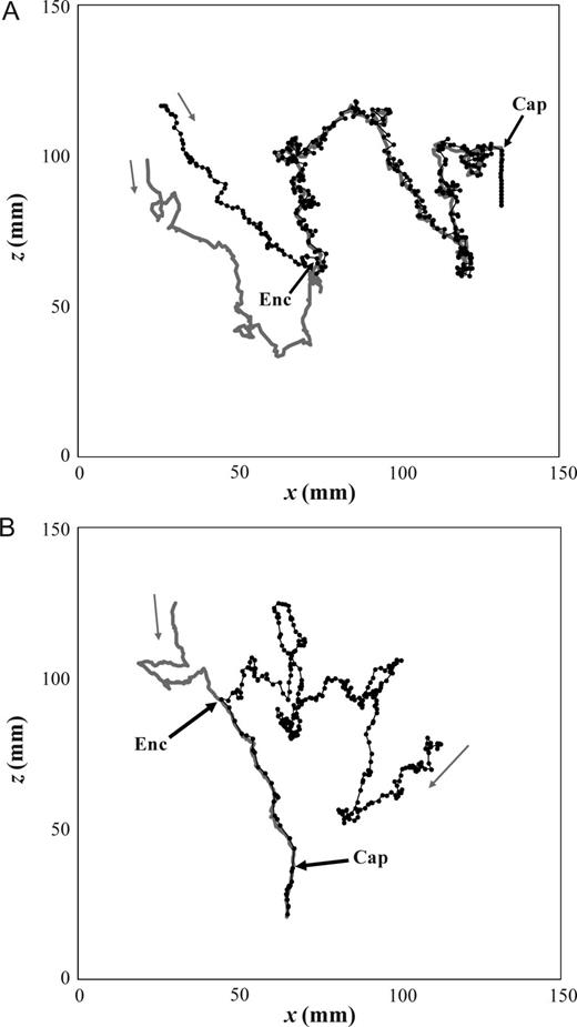
Two-dimensional illustrations of the mate-seeking behaviour of males E. affinis males following the trail of conspecific non-ovigerous females. The tracks of the females are shown in grey, and the tracks of the males in black, where the black dots represent positions plotted every 0.5 s. The grey arrows indicate the direction of motion, and the black arrows the locations where the male encounters the female trail (Enc) and successfully capture the female (Cap).
All the tracking events observed with ovigerous females (43) were initiated in the correct direction, 33 (76.7%) led to a mate contact and 10 led to loss of the trail after hops performed by females (Table II). None of the 33 contacts led to a capture, with ovigerous females consistently escaping upon contact with the male at a velocity ranging from 33.2 to 55.4 mm s−1.
Chemically and hydromechanically mediated perceptive distances
The distance  at which E. affinis males detected pheromone trails within 2.8–3.3 mm of the track line of non-ovigerous females and within 1.7–2.4 mm of the track line of ovigerous females. The direct linear distance
  between the male and the female at the initiation of mate pursuit behaviour ranged from 6.8 to 55.5 mm for non-ovigerous females and from 3.3 to 19.5 mm for ovigerous females (Table III). Males followed the trails of non-ovigerous and ovigerous females within 1.1–2.5 mm and 0.6 and 1.2 mm of the females track line (Table III). The hydromechanically mediated distances
  ranged from 1.2 to 2.3 mm and from 1.0 to 1.9 mm for males lunging at non-ovigerous and ovigerous females, respectively (Table III). The hydromechanically mediated distances
  ranged from 1.1 to 2.5 mm for males lunging at non-ovigerous females (N = 11) and 0.6 to 1.2 mm for males lunging at ovigerous females (N = 8; Table III).
Mate-seeking behaviour accuracy and efficiency
Eurytemora affinis males were more efficient in remotely detecting the trails of non-ovigerous females ( mm;
mm;  ) than those of ovigerous females (
 mm). The accuracy with which they followed ovigerous females (MFDR = 1.31 ± 0.04) was significantly lower (P < 0.05) than when following non-ovigerous females (MFDR = 1.12 ± 0.03). Males followed the trails of non-ovigerous females up to 22.3 s old over total tracking distances and tracking times up to 147.5 mm and 35.7 s, respectively; the trails of ovigerous females up to 12.1 s old were followed over total tracking distances and times of up to 45.3 mm and 13.7 s (Table III).
DISCUSSION
Cue-free swimming behaviour in E. affinis
Both the fraction of time allocated to different behaviour (cruising, hovering, breaking and sinking), and swimming and sinking speeds obtained in control experiments for E. affinis males, non-ovigerous females and ovigerous females are in the range of values previously reported for this species (Seuront, 2006, 2010c, 2012; Michalec et al., 2010; Bradley et al., 2013). Differences exist, however, between the swimming and sinking speeds reported in the literature (Table IV). As discussed elsewhere (Souissi et al., 2010; Seuront, 2010b; Dur et al., 2011a), these are likely to be the result of differences in rearing, acclimation and experimental conditions (Table IV). These discrepancies may, however, also come from author-related differences in the definition of a given behaviour. For instance, to my knowledge, this work is the first to separate the “swimming” behaviour of E. affinis into its “cruising” and “hovering” components; hence, the cruising speed reported here may differ from others. Similarly, despite the implicit definition of “passive sinking”, i.e. passive downward vertical motion, with tail down (see, for example, Tiselius and Johnson, 1990), some authors defined sinking speed as “a swimming speed between 1 and 8 mm/sec and a direction straight towards the bottom, when the copepod is not swimming but sinks slowly due to the influence of gravity” (Michalec et al., 2010; Cailleaud et al., 2011). Note that for sinking velocities of copepods of similar size to range between 1 and 8 mm s−1 as reported in Michalec et al. (Michalec et al., 2010) and Cailleaud et al. (Cailleaud et al., 2011), their density needs to vary by a factor of 8 or to violate the Stokes law, which would both be unprecedented in the zooplankton literature. It is much more likely that these very variable and high sinking speeds might, in turn, come from the confusion between “cruising” and “sinking” occurring when swimming behaviour is quantified based only on a two-dimensional projection of an intrinsically three-dimensional swimming behaviour (Dur et al., 2011a) and/or when the resolution of the video systems used are not sufficient to distinguish individuals actually passively sinking with their tail down from individuals actively swimming downwards (Seuront, 2012).
Literature review of the swimming and sinking speeds reported in the literature for E. affinis, together with the corresponding experimental conditions
| Swimming speed (mm s−1) | Sinking speed (mm s−1)a | 2D/3D | Salinity | Temperature (°C) | Density (ind.L−1) | Tank (cm3) | |||||
|---|---|---|---|---|---|---|---|---|---|---|---|
| M | NOF | OF | M | NOF | OF | ||||||
| Present studyb | 2.50 | 2.40 | 1.20 | 0.55 | 0.61 | 0.91 | 3D | 4 | 16 | 3 | 15 × 15 × 15 |
| Seuront (2006) | 1.10 | 1.11 | 0.31 | 0.45 | 0.46 | 0.80 | 2D | 0 | 15 | 25 | 20 × 20 × 5 |
| 1.12 | 1.15 | 0.38 | 0.43 | 0.45 | 0.79 | 2.5 | |||||
| 1.21 | 1.18 | 0.40 | 0.49 | 0.49 | 0.79 | 5 | |||||
| 1.38 | 1.40 | 0.45 | 0.46 | 0.47 | 0.77 | 10 | |||||
| 1.69 | 1.62 | 0.50 | 0.47 | 0.46 | 0.79 | 15 | |||||
| 2.46 | 2.37 | 0.66 | 0.46 | 0.46 | 0.80 | 25 | |||||
| 3.30 | 3.27 | 0.76 | 0.45 | 0.46 | 0.79 | 35 | |||||
| Woodson et al. (2007) | 2.81–4.87c | — | — | — | — | 2D | 26 | 12 | 2d | 100 × 30 × 30 | |
| Bradley et al. (2013) | 3.20 | 2.67 | — | 2.19 | 1.72 | — | 3D | 22 | 20–23 | 82–164 | 6 × 4.5 × 4.5 |
| Michalec et al. (2010)e | 3.34 | 1.74 | 2.47 | 1–8 | 1–8 | 1–8 | 2D | 0.5 | 20 | 66 | 5 × 5 × 6 |
| 2.84 | 2.37 | 2.97 | 1–8 | 1–8 | 1–8 | 5 | |||||
| 2.50 | 2.03 | 2.30 | 1–8 | 1–8 | 1–8 | 15 | |||||
| 1.87 | 1.87 | 2.12 | 1–8 | 1–8 | 1–8 | 25 | |||||
| Cailleaud et al. (2011) | 4.02 | 1.65 | — | 1–8 | 1–8 | 1–8 | 2D | 15 | 15 | 46 | 8.5 × 8.5 × 3 |
| Dur et al. (2011a, b)f | 1.77 | — | — | — | — | — | 2D | 25 | 23–25 | 40 | 5 × 5 × 5 |
| 1.69 | — | — | — | — | — | 25 | 19–22 | 80 | 5 × 5 × 5 | ||
| 1.00 | — | — | — | — | — | 25 | 20–23 | 120 | 5 × 5 × 5 | ||
| 1.62 | — | — | — | — | — | 25 | 19–21 | 160 | 5 × 5 × 5 | ||
| 1.54 | — | — | — | — | — | 25 | 20–23 | 40 | 10 × 10 × 10 | ||
| 1.38 | — | — | — | — | — | 25 | 19–21 | 40 | 15 × 15 × 15 | ||
| Seuront (2012) | 2.30 | 1.80 | — | 0.50 | 0.60 | — | 3D | 4 | 15 | 9 | 15 × 15 × 15 |
aAs the definition of sinking varies in the literature, it is stressed that it has been defined following its original definition (see, for example, Tiselius and Johnson, 1990), i.e. passive downward vertical motion, with tail down, in the present study, Seuront (2006) and Bradley et al. (2013). In contrast, Michalec et al. (2010) and Cailleaud et al. (2011) ambiguously defined sinking speed as “a swimming speed between 1 and 8 mm s−1 and a direction straight towards the bottom, when the copepod is not swimming but sinks slowly due to the influence of gravity”.
bNote that in the present work, swimming behaviour was split between cruising and hovering behaviours where copepods, respectively, swim with their rostro-caudal body axes aligned with the direction of motion, whether they were swimming up, down or horizontally, and swim upwards at slow speed in relatively linear directions with the rostro-caudal body axis oriented upwards and with frequent horizontal reorientation hops. None of the other studies reported here.
cAll behavioural experiments were conducted on mixed-sex copepods.
dBehavioural experiments were conducted in a 100 × 30 × 30 cm3 with 28–41 individuals, but behavioural observations were limited to a 10 cm × 10 cm observation window copepods were aggregated using a fiberoptic light source, resulting in 0–10 copepods being typically present in the observation window, with a mode of ca. 2.
eSwimming speed was graphically estimated from their Fig. 1.
fSwimming speed was graphically estimated from their Fig. 1a.
Cue-free versus pheromone-driven swimming behaviour in E. affinis
No significant differences were found between the control conditions (i.e. males swimming in GF/C filtered and autoclaved estuarine water) and both treatments (estuarine water conditioned with non-ovigerous and ovigerous females) neither in the proportion of time E. affinis males spent swimming, breaking and sinking (Fig. 3b) nor in their cruising and sinking speed (Fig. 4b). This agrees with observations conducted on males of the brackish copepod Pseudodiaptomus annandalei, who did not exhibit any significant change in their swimming speed between brackish water and female-conditioned brackish water (Dur et al., 2011b). This contrasts, however, with observations conducted on males of the freshwater calanoid Diaptomus leptopus and the marine pelagic copepod O. davisae who increased their swimming speed as a response to water conditioned with gravid females (Van Leeuwen and Maly, 1991) and to water conditioned with either virgin or mated females (Heuschele and Kiørboe, 2012). My observations may hence suggest a lack of chemosensory abilities in E. affinis males, at least towards conspecific pheromones as they have been recently shown to be extremely sensitive to (i) hydrocarbon concentrations orders of magnitude below lethal concentrations (Seuront, 2010a, 2012) and (ii) sublethal concentrations of nonylphenols (Cailleaud et al., 2011). However, the fractal dimension of the swimming trajectories of E. affinis males significantly increased from D = 1.39 ± 0.03 in control estuarine water to D = 1.48 ± 0.04 and D = 1.45 ± 0.02 in estuarine water conditioned with non-ovigerous and ovigerous females, respectively (Fig. 5b). This shows that E. affinis males perceive, and react to, the dilute smell of non-ovigerous and ovigerous females through a modification of the geometric complexity of their swimming patterns. The presence of the scent of conspecific females (either non-ovigerous or ovigerous) induces a modification in the search behaviour of E. affinis males. This confirms early suggestions that males can modify their motion behaviour as a response to female pheromones (Katona, 1973). Specifically, it is shown here that E. affinis males are able to modify their swimming behaviour in response to a diffuse background of pheromone concentrations.

 is the female density (Uttieri et al., 2007b). It is straightforward from Equation (4) that the observed increased in the fractal dimension of male trajectories between control estuarine water and estuarine water conditioned with either non-ovigerous or ovigerous females leads to the increased mate encounter rate. Note that Equation (4) has also been found for predatory copepods foraging in patchy food distributions (Cianelli et al., 2009), suggesting its applicability to both mating and predatory interactions, hence its generality. Recent results (Heuschele and Kiørboe, 2012) indicate that O. davisae males increase both their speed and directional persistence in water conditioned by virgin females. As this leads to a higher net distance travelled by males, this behaviour has been interpreted as a strategy to increase the chance to encounter a female, but also a predator (Heuschele and Kiørboe, 2012). In contrast, the development of a search intensive behaviour (i.e. high fractal dimension, hence low directional persistence) observed here for in E. affinis males in water conditioned by non-ovigerous and ovigerous females may be a way to decrease their hydromechanical conspicuousness for predator, while optimizing encounter rates in an environment carrying female cues. Both O. davisae and E. affinis are egg-carrying species that occur at relatively high density in estuarine environments, i.e. up to 500 ind.L−1 (Uye and Sano, 1995) and 250 ind. L−1 (Devreker et al., 2010). However, their feeding modes are fundamentally different and may account for the observed fundamental differences in their mate-searching strategies. In contrast to E. affinis, O. davisae is an ambush feeder; hence, males have to sacrifice feeding when searching for females (Kiørboe, 2007). The subsequent reduced feeding rate and the elevated risk of encountering predators related to their mate-search strategy may explain the much higher mortality of males than females and the subsequent strongly female-biased adult sex ratios in field populations of this species (Kiørboe, 2007). This is, however, not the case for E. affinis, who typically exhibit a male-biased sex ratio (Devreker et al., 2010). This suggests that the strong and weak direction persistence, respectively, reported for O. davisae (Heuschele and Kiørboe, 2012) and E. affinis (present work) are likely to bias predation pressure towards O. davisae males. The ability to distinguish between mated and non-mated females may save the males spermotophores and several hours per day of dangerous and energetically expensive fast female tracking (Kiørboe, 2007; Heuschele and Kiørboe, 2012) may be a selective advantage for an ambush feeder such as O. davisae. However, this ability is not as crucial for filter feeders such as E. affinis, who do not face the same constraints and hence develop distinct mate-searching strategies. It is also stressed that both E. affinis (present work) and O. davisae (Heuschele and Kiørboe, 2012) do not change their swimming behaviour in male-conditioned water, suggesting that both species have enough chemosensory abilities to distinguish male from female scent. This contrasts with observations conducted on T. longicornis (Yen and Lasley, 2010). This suggests a fundamental difference in the mating tactics and the use of spermatophores between different families of copepods, but also within the same family. While the resolution of this specific issue goes well beyond the objectives of the present study, further work is needed to unambiguously assess the evolutionary advantages of mate-searching strategies at play in copepods with fundamental species-specific intrinsic feeding strategies and motion behaviours. More generally, the properties of a search pattern (e.g. speed, directionality, space-filling) determine the success of a moving organism as a predator as widely exemplified for top predators such as sharks and seabirds (e.g. Humphries et al., 2010, 2012; Sims et al., 2011) and, in turn, the related potential susceptibility to predation as a moving target. This may also suggest that theoretical models showing that extensive search strategies are better than intensive ones when resources are scarce (Viswanathan et al., 1999, 2008, 2011) may not be as general as previously thought and might need to consider explicitly not only the search patterns of predators and the density and distribution of prey, but the actual motion pattern of the prey (or potential mate); see, for example, Visser and Kiørboe (Visser and Kiørboe, 2006) and Reynolds (Reynolds, 2006).
On the relevance of fractal analysis in copepod behavioural studies
These results confirm the strength of fractal analysis in detecting subtle differences in motion patterns that may be undetectable in standard behavioural variables (Coughlin et al., 1992; Seuront and Leterme, 2007; Seuront and Vincent, 2008; Seuront, 2010c, 2011b, 2012). This also demonstrates that a visual assessment of copepod trajectories may potentially lead to spurious conclusions. For instance, the differences in the complexity of E. affinis male and female swimming paths are visually far from trivial (Fig. 2), especially when comparing males (Fig. 2a) and non-ovigerous females (Fig. 2b). A qualitative visual assessment could have then legitimately, but erroneously (as the fractal dimensions of male swimming trajectories were significantly higher than those observed for non-ovigerous female; Fig. 5a), led to conclude to the absence of difference in the complexity of male and non-ovigerous female swimming paths. Results based on visual comparisons of swimming paths should hence be considered with extreme caution; for instance, a recent study assessing behavioural changes in males P. annandalei observed in brackish water and female-conditioned brackish water states that “the free motility patterns of males, visually identified, did not differ between the two water conditions” (Dur et al., 2011b). They did not, however, provide any objective quantification of the observed motility patterns. In a subsequent study of the effects of salinity on the swimming behaviour of P. annandalei, Michalec et al. (Michalec et al., 2012) describe the trajectories of males, ovigerous females and non-ovigerous females that are unambiguously visually distinct (see their Figure 7), as being “predominantly rectilinear”, “more convoluted” and “more tortuous” (hence implicitly fulfilling different degrees of space-filling). It may, however, be surprising, to both the fractal-oriented and fractal-naïve readers, that the space-filling properties of these trajectories were characterized by non-significantly different fractal dimensions. Note, however, that the above-mentioned visual comparison is quite ancillary to the main point of the papers mentioned, and any criticisms implied by the previous statements do not detract from the central point of their work.
In addition, the fractal dimensions reported in Michalec et al. (Michalec et al., 2012) often fall outside the theoretical range 1 ≤ D ≤ 2 expected for a swimming trajectory under each of the experimental conditions they have considered (see their Figure 8). Note that a few other studies report fractal dimensions falling outside the range 1 ≤ D ≤ 2, i.e. D < 1 (Dowling et al., 2000) and D > 2 (Coughlin et al., 1992; Shimizu et al., 2002). In the absence of both a detailed procedure related to the way these fractal analyses were conducted and a discussion of the observed discrepancy between empirical estimates and their theoretical bounds, this suggests potential flaws in their approach. These flaws are difficult to unambiguously assess, but may stem from a range of factors that are both extrinsic and intrinsic to fractal analysis such as the potential anisotropy and the different length of the analysed trajectories, and the goodness-of-fit used to characterize the range of scale over which the scaling properties of the trajectories (hence their fractal dimensions) are estimated; see, for example, Seuront (Seuront, 2010c) for a detailed discussion on the subject.
The differences observed in the present work between the fractal dimensions of the swimming trajectories of E. affinis males (D = 1.39 ± 0.03), non-ovigerous females (D = 1.27 ± 0.03) and ovigerous females (D = 1.11 ± 0.02) are consistent with the results obtained from (i) E. affinis males (D = 1.35 ± 0.01), non-ovigerous females (D = 1.32 ± 0.01) and ovigerous females (D = 1.12 ± 0.01) in GF/C filtered estuarine water at a salinity of 25 (Seuront, 2006), (ii) E. affinis males (D = 1.43 ± 0.08) and non-ovigerous females (D = 1.31 ± 0.08) in GF/C filtered estuarine water at a salinity 5 (Seuront, 2012) and (iii) T. longicornis swimming paths observed in GF/C filtered coastal waters (i.e. D = 1.32 ± 0.02 for males and D = 1.27 ± 0.02 for females; Seuront, 2011a). In contrast, the swimming paths of Oncaea venusta males and females were characterized by non-significantly different fractal dimensions, i.e. D = 1.14 ± 0.06 for males and D = 1.15 ± 0.06 for females, when investigated in natural seawater (Seuront et al., 2004d). The differences reported above between T. longicornis and E. affinis, and O. venusta may, however, be due to the presence and the absence of cues in their respective experimental set-ups. In the absence of cues, the different fractal dimensions estimated from male and female swimming paths in both T. longicornis and E. affinis may be related to intrinsic (i.e. innate) differences in male and female search strategies. Male fractal dimensions are significantly higher than female ones; hence, males are engaged in more intensive search strategies than females, which is consistent with the reported behaviour of males in the presence of female cues (e.g. Doall et al., 1998; Nihongi et al., 2004; Bagøien and Kiørboe, 2005a, b; Goetze, 2008; Goetze and Kiørboe, 2008; Yen et al., 2011; Seuront, 2011a). The similar complexity of the swimming paths of O. venusta males and females in natural seawater may be related to a common, hence sex-independent, adaptive behavioural strategy developed in response to the range of chemical cues (from, for example, prey, conspecifics and predators) that are likely to be present in their experimental containers. Note that the fractal dimensions of T. longicornis adult females observed in natural seawater range between D = 1.18 ± 0.04 and D = 1.82 ± 0.05, depending on the nature and abundance of the phytoplankton community and seawater viscosity (Seuront and Vincent, 2008). More generally, the fractal dimensions estimated from E. affinis female swimming paths observed in control estuarine water are in the range of values observed for females of different calanoid species investigated using the same experimental protocol as the present work, i.e. D = 1.25 ± 0.02 for Acartia clausi, D = 1.37 ± 0.03 for C. typicus, D = 1.27 ± 0.02 for Pseudocalanus elongatus, D = 1.42 ± 0.03 for Paracalanus parvus and D = 1.25 ± 0.03 for T. longicornis (Seuront, 2011b).
Trail-following behaviour in E. affinis
In addition to the observation that males of the estuarine copepod species E. affinis are able to modify their swimming behaviour in response to a diffuse background of pheromone concentrations, the present work shows that they follow trail mimics containing female scent (Table I). This demonstrates that a chemical signal can guide E. affinis males to conspecific females. This confirms early suggestion that male E. affinis can use pheromones to detect females (Katona, 1973). This is confirmed and generalized by subsequent observations of males swimming freely in a three-dimensional environment, who modify their direction of motion upon encountering the pheromone trails of females. Female trails up to 22 s old can be detected and followed over distances and durations of up to nearly 15 cm and 36 s, respectively. These observations indicate that males follow trail mimics in a manner similar to how they follow female copepods.
Eurytemora affinis males follow the trails of non-ovigerous and ovigerous females to the point of mate contact with very similar efficiencies (Table II). Their accuracy and efficiency to detect and subsequently follow pheromone trails are, however, consistently higher for non-ovigerous females (Table III). This suggests that males are more sensitive to the pheromone released by non-ovigerous females or that ovigerous females release less pheromones than non-ovigerous ones. This is consistent with previous studies suggesting that (i) pheromone attraction in copepods may stop after copulation (Lonsdale et al., 1998), (ii) the placement of a spermatophore may prevent the release of pheromones through the genital opening (Vigoni et al., 1999), in several copepods species the placement of the spermatophore sealed the genital atrium with a “mating plug” which can stay in place even after the spermatophore is removed (Anstensrud, 1990; Corni et al., 2001; Barthélémy et al., 2003), and (iii) males are able to distinguish between virgin and inseminated females (Uchima and Murano, 1988; Lazzaretto et al., 1993) through the detection of changes in the chemical composition of the female cues (Watras, 1983; Heuschele and Kiørboe, 2012). Note that the identification of the female mating status is also mediated by contact pheromones (Ting et al., 2000), which may explain why no capture was ever observed when males successfully tracked ovigerous females. The absence of escape behaviour exhibited by ovigerous females before mate contact may also suggest that in contrast to non-ovigerous females, ovigerous females do not have remote hydromechanical sensing abilities, but rely instead on surface sensors that may involve either chemoreception or mechanoreception (Frey et al., 1998; Kelly et al., 1998). Alternatively ovigerous females may not escape from males before contact to minimize useless energy expenditure, which interestingly implies that they have the ability to remotely differentiate the hydromechanical signature of a conspecific male from that of a potential predator.
The chemical trail-following behaviour described here for E. affinis is similar to the behaviour observed in other calanoid copepods such as T. longicornis (Doall et al., 1998; Goetze and Kiørboe, 2008; Seuront, 2011a), T. stylifera (Goetze and Kiørboe, 2008), C. typicus (Bagøien and Kiørboe, 2005a, b) and C. hamatus (Goetze, 2008). However, the tracking distance and trail residence time strongly vary between species and studies. For instance, Doall et al. (Doall et al., 1998) and Goetze and Kiørboe (Goetze and Kiørboe, 2008) reported males tracking females over distances of ca. 130 and 61 mm for up to 5.5 and 2.2 s, respectively. Temora stylifera males tracked female trails over 90.6 mm for 9.7 s (Goetze and Kiørboe, 2008). Similarly, C. typicus (Bagøien and Kiørboe, 2005a, b) and C. hamatus (Goetze, 2008) tracked the pheromone trails of conspecific females over distances of 170 and 41.4 mm for 5.7 and 9.6 s. In the present work, E. affinis males performed similarly, detecting pheromone trails up to 22.3 s old and tracking them up to 147.5 mm for 35.7 s (Table III).
Chemical versus hydromechanical cues in E. affinis mate detection
This work shows that male E. affinis can (i) react to background pheromone concentration and subsequently modify their swimming behaviour to optimize male–female encounter rates and (ii) use chemical trails to detect and track females. However, the male behaviour just before the final lunge and female capture suggests that hydromechanical cues are also used during the final phase of mate tracking. This is consistent with the similarity between the hydromechanically mediated distances  and
and  observed for males lunging at both non-ovigerous and ovigerous females (Table III) and suggests that E. affinis males hydromechanically detect females at similar distances whether they are trail-following them or swimming independently of the female pheromone trails. Note that E. affinis males follow unscented control trails and trail mimics conditioned with males at similar rates (9.3 and 9.4%; Table I), but never followed actual male trails and did not exhibit any behavioural changes in male-conditioned estuarine water. This suggests that in the trail-mimic experiment, males encountering unscented control trails and male-conditioned trail mimics likely reacted to the density difference present in the trail rather than to the actual scent of the trail. This is consistent with the responsiveness of a range of copepod species, including E. affinis, to physical gradients (Woodson et al., 2005, 2007, 2008). Note that the hydromechanically mediated distances
  and
and  are significantly smaller than the chemically mediated distances
  and
and  , typically 2- to 10-fold smaller (Table III). This indicates that the contribution of hydromechanical cues to the remote detection of female copepods may be relatively limited compared with the role played by chemoreception through pheromone trail tracking and limited to the final stage of a successful trail following and to the opportunistic encounter of a female. Further work is nevertheless needed on a range of copepod species to assess the relevance of the relative contribution of chemical and hydromechanical cues in determining mating encounters in the ocean.
Conclusions
This work shows that the estuarine copepod E. affinis relies on both chemical and hydromechanical cues to detect, track and eventually capture conspecific females. However, the surface ocean is mainly turbulent (Peters and Marrasé, 2002), and turbulence typically stretches, twists and breaks chemical trails (Visser and Jackson, 2004). Chemical trails start to erode for turbulent intensities above a critical dissipation rate of 10−9 m2 s−3 (Kiørboe et al., 2005) leading to more diffuse pheromone distributions. In coastal and estuarine waters where copepods flourish, turbulence intensities are typically in the range 10−6–10−4 m2 s−3 (Peters and Marrasé, 2002; Seuront, 2005) so pheromone trails are homogenized by turbulent diffusion and trail following is unlikely. As a consequence, the hydromechanically mediated distances reported in the present work, the ability of calanoid copepods to detect strain rates of 0.05–0.5 s−1 (Fields and Weissburg, 2005; Woodson et al., 2005), combined with the observed behavioural responses to a diffuse background of pheromone concentrations, might be a much more fundamental adaptation to mate finding than tracking the pheromone trail.
FUNDING
This research was financially supported by the Australian Research Council's Discovery Projects funding scheme (projects number DP0664681 and DP0988554), Flinders University, the Centre National de la Recherche Scientifique (CNRS) and the South Australian Government through the Marine Innovation South Australia Initiative. Professor L.S. is the recipient of an Australian Professorial Fellowship (project number DP0988554).
ACKNOWLEDGEMENTS
D. Devreker, G. Dur, H.-J. Hwang, F.G. Schmitt and S. Souissi are acknowledged for the numerous discussions that motivated the present work. N. Spilmont is acknowledged for stimulating discussions on this topic.
REFERENCES
Author notes
Corresponding editor: Roger Harris
