


Abstract
Electron–positron pair production by collision of photons is investigated in view of application to pulsar physics. We compute the absorption rate of individual gamma-ray photons by an arbitrary anisotropic distribution of softer photons, and the energy and angular spectrum of the outgoing leptons. We work analytically within the approximation that 1 ≫ mc2/E > ε/E, with E and ε the gamma-ray and soft-photon maximum energy and mc2 the electron mass energy. We give results at leading order in these small parameters. For practical purposes, we provide expressions in the form of Laurent series which give correct reaction rates in the isotropic case within an average error of ∼ 7 per cent. We apply this formalism to gamma-rays flying downward or upward from a hot neutron star thermally radiating at a uniform temperature of 106 K. Other temperatures can be easily deduced using the relevant scaling laws. We find differences in absorption between these two extreme directions of almost two orders of magnitude, much larger than our error estimate. The magnetosphere appears completely opaque to downward gamma-rays while there are up to ∼ 10 per cent chances of absorbing an upward gamma-ray. We provide energy and angular spectra for both upward and downward gamma-rays. Energy spectra show a typical double peak, with larger separation at larger gamma-ray energies. Angular spectra are very narrow, with an opening angle ranging from 10−3 to 10−7 radians with increasing gamma-ray energies.
1 INTRODUCTION
Electron–positron pair creation by collision of two photons, also called Breit–Wheeler process, is important in a series of astrophysical questions (Ruffini, Vereshchagin & Xue 2010). Amongst them is the filling of recycled pulsar magnetospheres with plasmas.
The cross-section of two-photon-pair creation has been derived in Berestetskii, Lifshitz & Pitaevski (1982). This is a function of the four momentum of both electrons. In pulsar magnetospheres, there is generally a huge reservoir of low-energy photons and a small number of high-energy photons. In order to decrease computational cost compared to pairwise calculations, the cross-section is integrated over the distribution of the low-energy photons. The exact formula for the reaction rate on an isotropic soft-photon background was first derived in Nikishov (1962) to estimate the absorption of gamma-rays by the extragalactic background light. Numerical integration was needed to obtain practical results. In contexts such as active galactic nuclei or X-ray binaries, various formulations and approximations were developed. Approximated analytical expressions were given in Bonometto & Rees (1971) and Agaronyan, Atoyan & Nagapetyan (1983) in the case of an isotropic soft-photon background distribution and averaging over outgoing angles of the produced leptons. The expression of Agaronyan et al. (1983) also applies for a bi-isotropic photon distribution (both strong and weak photon distributions are isotropic) without angle averaging over leptons. In these papers, the authors provide the energy spectrum of the outgoing leptons. An exact expressions in the case of bi-isotropic photon distribution is derived in Boettcher & Schlickeiser (1997), as well as a comparison to the previous approximations that favors the approach in Agaronyan et al. (1983) for its better accuracy.
The standard picture of a pulsar magnetosphere assumes that its inner part is filled with plasma and corotates with the neutron star with angular velocity Ω*. The primary plasma is made of matter lifted from the neutron-star surface by electric fields (Goldreich & Julian 1969). These particles have highly relativistic energies; their motion in the neutron-star magnetic field generates synchrotron and curvature gamma-ray photons. In addition to primary particles, Sturrock (1971) has shown that electron–positron pairs are created in or near the acceleration regions of the magnetosphere. This provides plasma capable of screening the electric field component parallel to the magnetic field. There are two processes of pair creation: two-photon process and one-photon process in the presence of a strong magnetic field. The one-photon process is the most efficient with young and standard pulsars, of which magnetic field is in the range B ∼ 106–108 T (Burns & Harding 1984). The photon–photon pair-creation process can become more important with high-temperature polar caps, and when the magnetic field is below 106 T as in recycled pulsar magnetospheres. Anisotropy of the soft-photon sources is prone to be important as they are expected to come either from the star (hot spots) or from synchrotron radiation in magnetospheric gaps. That is the main reason of our present investigation.
Many detailed studies of pair-creation cascades in pulsar magnetospheres are based only on the one-photon process. This is for instance the case in the recent studies in Timokhin & Harding (2015). Others take the two reactions into account (Chen & Beloborodov 2014; Harding, Muslimov & Zhang 2002).
In numerical simulations of pulsars, the pair-creation rate is generally estimated with simple proxies. For instance, in Chen & Beloborodov (2014), a mean-free path l = 0.2R* is used for the one-photon process, and l = 2R* for the two-photon process. The rate of creation of pairs is not explicited as a function of the electron (or positron) momentum, neither of the local photon background. Instead, pair creations are supposed to be abundant enough to supply electric charges and current densities. The authors write that this approximation is somehow similar to the force-free approximation. In Harding et al. (2002), both one-photon and two-photon processes are taken into account, and the two-photon process is controlled by a mean-free path derived from Zhang & Qiao (1998), where anisotropy is partially taken into account : the energy integral has a lower limit that depends on the angular size of the hot cap providing the soft-photon background. Besides, these authors do not provide spectra for the created pairs although the energy distribution of the outgoing particles are important for the dynamics of pair cascades. A more complete model needs an integration over every local surface element with a threshold that depends on the location of each elementary emitter. This is what the results of the present paper allow us to do within some approximation, together with angular and energy spectra of the outgoing pairs.
Pair creation by two photons is also important in high energy gamma-ray astrophysics. Many papers about gamma-ray bursts and active galactic nuclei refer to Svensson (1987) and the integrated mean-free path in this paper is also based on Nikishov (1962). Actually, spectra of TeV radiation observed from distant (beyond 100 Mpc) extragalactic objects suffer essential deformation during the passage through the intergalactic medium, caused by energy-dependent absorption of gamma-rays interacting with the diffuse extragalactic background light (Nikishov 1962; Gould & Schréder 1966). This effect drastically limits the horizon of the gamma-ray universe, and this has been taken into account in the science case of high-energy gamma-ray observatories (Vassiliev 2000).
In this paper, we revisit the computation of the two-photon pair-creation rate with the aim of dealing with arbitrarily anisotropic soft-photon background distribution. In addition, we give formulas for angle and energy spectra in order to be able to determine in which state pairs are created. After an introduction to the two-photon pair creation equations in Section 2, the integral over the low-energy photons is defined in Section 3. Practical expressions for spectra are derived in Section 4, and applications to the cosmic microwave background and to a hot neutron star are developed in Section 5.2.
2 THE TWO-PHOTON-QUANTUM- ELECTRODYNAMICS REACTION
When not specified, we use a unit system where the speed of light c = 1.
2.1 General formalism
The state of a free photon can be decomposed on a plane-wave basis parametrized by four momentum and polarization. The common assumption is that the effective state of a photon is very well approximated by one plane wave at the time of the encounter. Such a state is not physical in itself, because it cannot be normalized, i.e. it does not belong to the L2 space, or more physically because the Heinsenberg inequality imposes to the wavefunction to be entirely spread through space as a consequence of the perfect determination of momentum. Though, this assumption should be valid over a local four-volume of space–time Vδt, where the interaction through operator |$\hat{S}$| takes place.
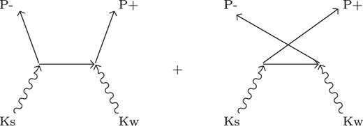
Reaction of electron–positron pair creation from a pair of photons represented to first order by Feynman diagrams. Photons have four-momenta Ks and Kw while electron and positron have, respectively, P− and P+.
A few important properties of dw can be evidenced by taking a look at cross-section (6) averaged over every possible direction of the outgoing lepton (Berestetskii et al. 1982). As a result, the averaged cross-section depends only on the kinematic invariant τ = t/(4m2) the ratio between the CM energy and the threshold energy. Without loss of generality in the present discussion, we can assume that the reaction takes place in the CM frame, such that the elementary current j = 2/V. The ultra-relativistic limit (Berestetskii et al. 1982) shows that the cross-section vanishes like log τ/τ. This kind of decrease with energy is a common feature of quantum mechanical cross-sections. Moreover, one can numerically estimate the CM energy corresponding to the maximum of the reaction rate to be |$\sqrt{t} \simeq 1.4(2m)$|.
Concerning the angular dependency, leptons are created almost isotropically when the reaction is near threshold while their momenta become aligned with those of the progenitor photons when going to higher energies (see e.g. Berestetskii et al. 1982). In the observer's frame, this translates in a larger angular dispersion for reactions close to threshold.
Equations (3–8) fully describe the interaction for a given pair of photons; but in a pulsar's magnetosphere, there is a huge amount of photon pairs. In a simulation, it is not possible to compute dw for each pair; we need a statistical approach and a kind of ‘collective’ reaction rate dw. We define it in the next section.
2.2 The pair reactions that count in a pulsar magnetosphere
In a pulsar magnetosphere, the weak photons Kw are mostly caused by the blackbody radiation of the neutron star, or possibly by synchrotron from secondary pair cascades. Their energies range in the X-ray domain. The strong photons are caused by the synchro-curvature radiation of energetic particles (electrons, positrons and possibly ions). Their energies are in the gamma-ray domain. They are more scarce than weak photons. Let's follow a ‘rare’ high-energy, strong photon taken from a phase-space distribution fs. We assume that it flies through an abundant stream of low-energy, weak photons with a distribution fw.
Strong photons negligibly interact with other strong photons because they are not abundant, and because the reaction would likely be far above threshold in equation (10), and therefore inefficient.
Weak photons do not interact with other weak photons since their energies are under the reaction threshold.
3 PROBABILITY OF REACTION FOR A GIVEN PHOTON DISTRIBUTION
3.1 The domain of integration
4 GENERAL SOLUTION
4.1 Energy spectrum
4.2 Angular spectrum
It is also possible to compute the angular spectrum of the outgoing leptons. The problem has to be split in two, whether one consider the higher energy particle (p > k/2) or the lower-energy particle (p < k/2).
In virtue of 37, Fw now depends explicitly on p, hence the dependence in (41).
4.3 With conic boundary conditions
To obtain the final spectrum (58) (resp. 60), integration over μ (resp. over p) is possible analytically: the first line of (63) is a rational fraction that can be integrated through partial fraction decomposition and the second line yields expressions of the type ∫xklog (polynomial(x))dx (where k is integral) which values are given in most relevant textbooks such as (Gradshteyn et al. 2000). However, the resulting expressions may be lengthy and a direct numerical integration might sometimes be more efficient.
5 APPLICATIONS
5.1 Isotropic blackbody background distribution
![Spectra of outgoing leptons (electron or positron) for different strong-photon momenta k on a blackbody background at temperature Tbb (top panel). m is the mass of the electron, the speed of light and the Boltzmann constant are taken to be unity. The amplitudes are normalized to the amplitude of the peaks of each spectrum, and these amplitudes are reported on the lower panel. As in Fig. 2, these amplitudes are normalized to correspond to the cosmic-microwave background. The most intense peaks arise around a momentum k such that its reaction with a background photon at Tbb is at threshold, i.e. kTbb ∼ m2. The more above threshold, the more separated, narrow and low the peaks are. The separation of the peaks can be understood as a mere relativistic-frame effect, by analogy with a two-photon collision. [A color version of this figure is available online.]](https://oup.silverchair-cdn.com/oup/backfile/Content_public/Journal/mnras/474/2/10.1093_mnras_stx2658/2/m_stx2658fig2.jpeg?Expires=1716316473&Signature=jUUE2QTiQvQ0FGtxR-uKxElhCcYelhOkHeAr-8Qojp~kHGDrKOicT1XmhJy5kKo5LiFBhnnURRCHwoQWgLNiBhVhfqH690P5Wf0itEVSY9zqA9QcyQ2IEtP2UsVc5TqDb9FyQrdMZs9mt4gj3vQbSTQtpjZFME4aoXpRDRU~O4Yp4EXcwb9-1Zz2YUFnnaqQvzd7OIO4FWRKjr2vvNARkOjn~qxOdvEVKC86wt-x~wwsUQyWiSS-uxtkBaYEt26GhNV~CeHuz~pwVwIaKKaFa0VugPaMTAGm9mE-RBn06lVKZmKMOQw7Ffl91S6zU11mFdubu~ZVDzkHe0Z35ayP0w__&Key-Pair-Id=APKAIE5G5CRDK6RD3PGA)
Spectra of outgoing leptons (electron or positron) for different strong-photon momenta k on a blackbody background at temperature Tbb (top panel). m is the mass of the electron, the speed of light and the Boltzmann constant are taken to be unity. The amplitudes are normalized to the amplitude of the peaks of each spectrum, and these amplitudes are reported on the lower panel. As in Fig. 2, these amplitudes are normalized to correspond to the cosmic-microwave background. The most intense peaks arise around a momentum k such that its reaction with a background photon at Tbb is at threshold, i.e. kTbb ∼ m2. The more above threshold, the more separated, narrow and low the peaks are. The separation of the peaks can be understood as a mere relativistic-frame effect, by analogy with a two-photon collision. [A color version of this figure is available online.]
![Comparison of absorption of high-energy photons on a blackbody background with Nikishov's formula (dashed line) and with our's (VMB, plain line). The scaling (66) is that of a blackbody at Tbb = 2.7 K (see formula 66) to give an estimate of the effect of the cosmic-microwave background. In this case, the energy of the strong photons ranges between k ∼ 100 TeV and k ∼ 108 TeV. The bottom panel shows the ratio between the two theories. The ratio of probabilities averaged over k is about 1.07. The peak of our curve occurs around 2.6m2/T while Nikishov's is around 1.9m2/T. The ratio between the two curves at the position of our peak is approximately 1.01. [A color version of this figure is available online.]](https://oup.silverchair-cdn.com/oup/backfile/Content_public/Journal/mnras/474/2/10.1093_mnras_stx2658/2/m_stx2658fig3.jpeg?Expires=1716316473&Signature=TmrVgJcycGjdvPSCJszKRo6hbeqkF10B0ElYKMQe2PRELKLKDugj6Uv4AbV0pbjWakc-iIJlCsHnyGnQ8x02JMA1t6i19eA9d~8qCFQirYRQcaifLki9XqOvSTzoVakIdv5jY5Tv5Pw1~uOXlt1XJzc6~3geXpMxvkk6xWXxBBQEYjXxIdvllMfzbmh71QyZxszKvVOBepGQYPTcySfYXGPzDNuZC03MHpx9ys1kpHPVWCx8EW-bhve0wDEgQpkzfBe4iAPLNIAoAYSZg8ceVFJy--77jPeqfxkqw7DnsZ9APCtLlQISz8V3riaEgQFRj2vhZRc7HFq851iH-IH9Eg__&Key-Pair-Id=APKAIE5G5CRDK6RD3PGA)
Comparison of absorption of high-energy photons on a blackbody background with Nikishov's formula (dashed line) and with our's (VMB, plain line). The scaling (66) is that of a blackbody at Tbb = 2.7 K (see formula 66) to give an estimate of the effect of the cosmic-microwave background. In this case, the energy of the strong photons ranges between k ∼ 100 TeV and k ∼ 108 TeV. The bottom panel shows the ratio between the two theories. The ratio of probabilities averaged over k is about 1.07. The peak of our curve occurs around 2.6m2/T while Nikishov's is around 1.9m2/T. The ratio between the two curves at the position of our peak is approximately 1.01. [A color version of this figure is available online.]
Fig. 3 shows the pair-creation spectra for different values of ζ. Those spectra are directly computed using equation (38) and expressed as a function of p/k which allows the same scaling law as in equation (66), with p the momentum of one of the created leptons, and normalize each spectrum to unity such that the obtained spectral shape are universal, i.e. do not depend on the temperature of the blackbody or on the absolute value of k, but only on ζ. The shape and evolution of the spectra with the strong-photon energy is consistent with Agaronyan et al. (1983). In this paper, the authors consider spectra resulting from the reaction of two isotropic monoenergetic photon distributions with energies ε and k that are symmetrical with respect to (k + ε)/2. Here, every spectrum is symmetrical with respect to p/k = 0.5 as a result of neglecting ◯(ε/k) terms. Besides the shape of these spectra is very reminiscing of pair-creation in the photon-plus-magnetic-field process that is well known in the field of neutron-star magnetospheres (Daugherty & Harding 1983). The analogy is not fortuitous since the latter process can in principle be seen as the interaction of a strong photon with an assembly of magnetic-field photons. We see in Fig. 3 that each spectrum is made of two peaks that move apart and become narrower and weaker as the reaction occurs farther above threshold. Note that the narrowing is relative to the momentum span and not absolute.
The separation of the peaks at higher energies results from the fact that the cross-section favors alignment of ingoing and outgoing particles in the CM frame if the energy is much larger than the threshold energy. It follows that a Lorentz boost to the observer's frame along this axis results in a low-energy and a high-energy particle. The intensity of the peaks of course depends on the background distribution, but also on the cross-section which decays as log (τ)/τ (see Section 2.1). The latter dependency explains the above-threshold decrease of the peak intensity and the former explains the below-threshold decrease, as shown on the lower panel of Fig. 3. One notices that spectra are not smooth in their centre, which is naturally explained by our approximations that ensure continuity at the centre but not continuity of derivatives.
5.2 Above a hot neutron star
In this section, we consider a homogeneously hot neutron star at temperature T and two kinds of photons: the down photons and the up photons. Down photons are going radially towards the centre of the star while up photons are going in the opposite direction, away from the star. This configuration aims at approximating a pulsar magnetic pole. Indeed, in a pulsar magnetosphere high-energy photons are expected to be mostly created by curvature radiation of electrons and positrons flowing along magnetic field lines that can be considered radial at low altitudes above the poles. Note that we do not consider only a hot cap here but the full star, as means of geometrical simplification.
The case of pair production from photon–photon collisions in pulsar magnetospheres was studied by authors such as Zhang & Qiao (1998) and Harding et al. (2002). In these papers, the authors generalize the formula of Nikishov (1962) with a minimum energy threshold for the background distribution corrected by a factor (1 − cos θc)−1, where θc is the maximum viewing angle on the hot polar cap of the star. In other words, they consider an isotropic blackbody distribution where only photons within the viewing angle of the cap contribute, however with a threshold energy that corresponds to the largest incidence angle only since the threshold does not depend on the location of the emitter on the cap. Therefore, this approximation overestimates the threshold which generally translates in underestimating the reaction rate. This has little consequences when the viewing angle is wide, which is the case very close to the cap. However, one expects a faster decrease as one goes away from the cap and the factor (1 − cos θc)−1 grows larger. As an example, the authors of Zhang & Qiao (1998) compute a maximum reaction probability of 5.7 × 10⁻⁵ m−1 at a viewing angle of 90° when we get 6.7 × 10⁻⁵m−1 (see peak of the down-photon h = 10−3 curve on Fig. 5 for an estimate), but they obtain only 6.3 × 10⁻⁶ m−1 at 45° when we still have a probability of 4.3 × 10⁻⁵ m−1 (see their equation 9, for T = 106 K).
Besides, an interest of our formalism is that it can in principle deal with any other orientation of the strong photon with respect to the star, and in particular the up photons.
![A neutron star of centre O and radius R* above which an up photon and a down photon are represented by radial arrows of opposite directions. Both photons are represented at a height h above the surface of the star. From this height, they can interact with soft photons coming from the surface of the star within a cone of aperture ξhorizon, equation (69), represented by dashed lines. The incidence angle between the strong photon and soft photons therefore lies between 0 and ξhorizon for the up photon (purple upward arrow), and between $\pi - \xi _\mathrm{horizon}$ and π for the down photon (blue downward arrow). [A color version of this figure is available online.]](https://oup.silverchair-cdn.com/oup/backfile/Content_public/Journal/mnras/474/2/10.1093_mnras_stx2658/2/m_stx2658fig4.jpeg?Expires=1716316473&Signature=zfqzGvUH0UZb-bHpTlBH9~hJH5Z5JNibvytRQYEiyO-P6KJD2OwiZqqSARuzFnWL79aUOfZ0MisJOS-f-eaMhfNg6zLSvczSbZ6mWjomXR6YmT7Wl6X6XqgadlrDqc387TANeDSguDyGoM81zRYnD8ltHWet6F5je~~cxM-06r6E7nfq7c20zFzK2U1zVtoyxfs72s3hULdxyPDJodTrAI8xL0Huoobgk10IFwmnfQbYHjNLCdtX8fpp4nZUHg3BT5cu1~okZqi0hXf6A5cyc4CsDVMuDnludSWsk5AxxU9Mxo09OnaCmUWnrm3EEmG54XcRB-3-3335D1oBV4~MHg__&Key-Pair-Id=APKAIE5G5CRDK6RD3PGA)
A neutron star of centre O and radius R* above which an up photon and a down photon are represented by radial arrows of opposite directions. Both photons are represented at a height h above the surface of the star. From this height, they can interact with soft photons coming from the surface of the star within a cone of aperture ξhorizon, equation (69), represented by dashed lines. The incidence angle between the strong photon and soft photons therefore lies between 0 and ξhorizon for the up photon (purple upward arrow), and between |$\pi - \xi _\mathrm{horizon}$| and π for the down photon (blue downward arrow). [A color version of this figure is available online.]
Fig. 5 shows the probability of reaction per unit length (we will sometimes say ‘reaction rate’) as a function of ζ at various heights h above the cap (left-hand panel), and as a function of h at various ζ (right-hand panel). As in the previous subsection, the temperature dependance is T3 for a given value of ζ. All the figures in this section are made with a fiducial temperature of 106 K. With this value, the conversion from ζ to k is: k ≃ 5.9 × 10³ζmc2. At the lowest altitude we computed, h = 10−3R*, the peak of the reaction rate is around ζ = 1.6 for down photons and about an order of magnitude higher for up photons ζ ≃ 16. This is a direct consequence of the threshold equation (67) given the less favourable incidence angles of up photons. Another point is that the position of the maximum shifts to lower ζ as height increases for down photons, but to larger ζs for up photons. As can be seen on the right-hand-side panel, the reaction probability per unit length is fairly stable (within a factor of two) until ∼1R*, after which it decays very sharply. The decay is sharper as ζ increases for down photons and smoother for up photons, which explains the crossing between some curves on the right-hand-side panel.
![Probability of reaction per metre of a strong photon of momentum k as a function of ζ = (kkBT)/mc2)2 and height h above a star of radius R*. Up-triangle markers represent photons going radially up from the star. Down-triangle markers represent photons going down to the star. The probability scales like T3, according to equation (66), and is here represented using a fiducial T = 106 K. Left-hand-side panel: probability as a function of ζ at various heights. Right-hand-side panel: probability as a function of height h at various ζ. [A color version of this figure is available online.]](https://oup.silverchair-cdn.com/oup/backfile/Content_public/Journal/mnras/474/2/10.1093_mnras_stx2658/2/m_stx2658fig5.jpeg?Expires=1716316473&Signature=XIJXy~-bG00zbtclW4OJLlGCEppeXOr5GeanGE2LQk3fWcLQwFglrAZY2a9P5gSsSH0Zp1lEer8UwbJtbL2rvlP7QA-IEJ3TKyqHzvoKOFxms7Uhh6P0zDC5k1KqUsVGnfZnwpT985REUtrLfrrO4PnrAg3aVMgeqsM-bPEgl2A29TMmx38yNhYCER~sQuSnA9mNWtRZJ~KxfLGuYTH8W40HQ7Q0N6vk4v4JS29-nEmet49PowEK3YzdZYA8mrW4UgKIgyGXnd8vMzEPJDaqyfiC4ycKCNsCdRlhkIIrtghRkbcNPKfj9Vaa85ipFcQnYiFjRU9h7degQ8MCTrpWZw__&Key-Pair-Id=APKAIE5G5CRDK6RD3PGA)
Probability of reaction per metre of a strong photon of momentum k as a function of ζ = (kkBT)/mc2)2 and height h above a star of radius R*. Up-triangle markers represent photons going radially up from the star. Down-triangle markers represent photons going down to the star. The probability scales like T3, according to equation (66), and is here represented using a fiducial T = 106 K. Left-hand-side panel: probability as a function of ζ at various heights. Right-hand-side panel: probability as a function of height h at various ζ. [A color version of this figure is available online.]
A qualitative reasoning explains these behaviours. For a low-energy down photon (i.e. ζ ≲ 1), most of the soft photons most likely to react are in a narrow cone almost face-on with the strong photon. The aperture of the cone defines the limit beyond which the reaction is below threshold. When the strong photon is higher, the almost face-on soft photons are the last to disappear because of the shrinking of the viewing angle. As energy rises, this cone becomes wider since soft photons provoking a near-threshold reaction are located at a wider angle according to formula (67). Inside the first cone also appears a co-axial cone with a narrower aperture inside which photons are not contributing significantly anymore, since reactions are too far above threshold (and therefore the cross-section is too small) because of small incidence angles. At large strong-photon energies (ζ ≫ 1), the soft photons close to the outer cone are the first to disappear when the viewing angle shrinks because of a larger height. This explains the faster decay of the reaction probability with h for larger ζs of down-photon curves on Fig. 5. The same kind of reasoning applies for up photons. Because soft photons are arriving ‘from behind’, there is always an inner cone inside which the reactions are below threshold, and an outer cone limited by the angle beyond which the cross-section is too small if ζ ≫ 1 or the viewing angle of the strong-photon energy is small enough. The lower the energy of the strong photon the wider the outer cone and the most sensitive to viewing angle the reaction rate is. That explains why, contrary to down photons, the reaction rate decays slower with altitude when ζ is larger in Fig. 5. With this reasoning, one also understands why the energy of the reaction-rate peak (left-hand panel) is quite stable at low altitudes and becomes smaller for down photons at high altitudes (≳1R*) or larger for up photons.
![Reaction rate in equation (28) integrated from 0 to 10R* for up and down photons as a function ζ. The amplitudes are valid for a homogeneously hot star of temperature T = 106 K, and can be converted to other temperatures using the T3 scaling law (66). For photons going down towards the star, the peak is at ζ ≃ 1.4 with an amplitude of ≃8.8. For photons going up away from the star, the peak is at ζ ≃ 30 with an amplitude of ≃0.23. [A color version of this figure is available online.]](https://oup.silverchair-cdn.com/oup/backfile/Content_public/Journal/mnras/474/2/10.1093_mnras_stx2658/2/m_stx2658fig6.jpeg?Expires=1716316473&Signature=JPYoynAqYKme4b6nohW1WxiafyXqZRpnrUa8TBebSBFP-Zruwv47jOulK5iG2SHb1SABD6ocsyf-ftQQgN7IUX2dDPTv~7QH~7AhGIkIST3Mv-0OR2Dzsk8k4t6oRD4kPd7IbnoY-XW8qjPd6vs7~5700gc1Yh2H1A3V8~J1iqW1M~YWQ~a55~P24tXnsQbiZb47mGrPxN8egTmkMHsT0GS94yjmyV4x44-qWfdRUidI05o31kwrkMOyf9AuOQgzIjilpkA5IQjL3NUjRydwH92R96u1Hjf7pqKNHbLJ3mBhys-mMzg2fD~Nll7rEDgy1GgQ-0xUWuTncSAeQOnlhQ__&Key-Pair-Id=APKAIE5G5CRDK6RD3PGA)
Reaction rate in equation (28) integrated from 0 to 10R* for up and down photons as a function ζ. The amplitudes are valid for a homogeneously hot star of temperature T = 106 K, and can be converted to other temperatures using the T3 scaling law (66). For photons going down towards the star, the peak is at ζ ≃ 1.4 with an amplitude of ≃8.8. For photons going up away from the star, the peak is at ζ ≃ 30 with an amplitude of ≃0.23. [A color version of this figure is available online.]
Fig. 7 shows the energy spectra of the created leptons (left-hand panel) and the evolution of the position and widths of the peaks as a function of ζ at various heights (right-hand panel). The spectra have the same double-peaked structure as in the isotropic case (Fig. 3) but evolve differently depending on the orientation of the strong photon. The general principle is the same: the more above threshold the more separated peaks, with the consequence that they narrow when they get close to the limits of p/k ∈ [0, 1]. For down photons, the width of the peaks wp (in unit of k) has very little dependence on altitudes which is due to the fact that for the range of ζ ≲ 20 visible on this plot (right-hand panel), the efficient soft photons are mostly face-on and suffer no effect of viewing angle. The same thing applies for the position of the most energetic peak pp (and the least energetic at k − pp). Down-photon peaks are wide wp ∼ 0.45 for ζ ≲ 2 and then sharply narrow while their position smoothly goes from pp/k ∼ 0.8 to pp/k ≲ 1 at large ζs. On the contrary, up photons are very sensitive to altitude, which is explained by the fact that the higher above the star, the narrower the viewing angle and therefore the incidence angle, and the more energetic up photons need to be for the reaction to be at or above threshold. As a consequence up-photons peaks are very centred at low values of ζs, with pp/k ∼ 0.6, and are even more centred at higher altitudes. With ζ rising, the energy distribution becomes increasingly asymmetric as pp/k → 1−, although it takes a larger ζ at higher altitude. Similarly, peak widths are growing with ζ until a maximum wp ∼ 0.45 at a ζ all the more large that altitude is high, after which wp drops sharply. This sharp change of slope happens because the two peaks separate (see comment of Fig. 7).
![Left-hand-side panel: example of two normalized spectra of energy of created particles. These spectra are normalized to the amplitude of the largest peak, and the energy in abscissa is normalized to the energy of the incident strong photon k. In both cases, k corresponds to ζ = 10 at an altitude h = 0.5R*, and the only difference resides in the up or down orientation of the strong photon. As in the isotropic case 3, spectra are generally made of two peaks more or less thin and separated. The width at half-maximum of peaks wp is defined in the two possible cases: if one side of a peak never reaches its half before rising again to another peak in which case the width is taken to be half of the double-peak width, or if the peak is well defined on both sides in which case the definition is straightforward. The position of the most energetic peak pp/k is defined as well. Right-hand-side panel: evolution with ζ of positions pp/k of the higher energy peak (curves on the higher part of the plot), and widths at half-maximum wp (curves on the lower part of the plot) for up and down photons at various heights h (in units of R*). Positions are ranging from 0.5 at low ζs which corresponds to a perfectly centred peak or to a null spectrum when a reaction is below threshold (lowest energies of up photons), to ≃0.98 at large ζs. The horizontal dotted line shows the positions at which the ratios between the two peaks is 10. Widths at half-maximum are rising to ∼0.45 until the two peaks separate and drop sharply to ≃0.029. [A color version of this figure is available online.]](https://oup.silverchair-cdn.com/oup/backfile/Content_public/Journal/mnras/474/2/10.1093_mnras_stx2658/2/m_stx2658fig7.jpeg?Expires=1716316473&Signature=leSJ~RPjTB0VA1ynEGuOhJ3~zyF3CCsqimIEpDrG-iPqHIhMyw8d7synuHnBUHQUKY97LjUpYuvSJOdwZLEsZXI-m0pAgeOsCbtMLTtinI41LuoUYN2X8dY138aRFijMR9mIsGnT8Nn4zXau~W5Ihb6NPsF6CNBpp6tQ3FdaW~MO35iw-dreIJpl6eruj1RpJNaB376PWrFT-igElOKW6K4k1p28EJrUT9vgzgUTDnmMUurGh2F-snsgSXYtTjqhRVVehFToR~YtFZIaQFN75BmlcDq2DitTybS-idchlwkgSxXT1Y68vvgqE3ymwX8A28NAMMpZIe1H2ItNF7cHEg__&Key-Pair-Id=APKAIE5G5CRDK6RD3PGA)
Left-hand-side panel: example of two normalized spectra of energy of created particles. These spectra are normalized to the amplitude of the largest peak, and the energy in abscissa is normalized to the energy of the incident strong photon k. In both cases, k corresponds to ζ = 10 at an altitude h = 0.5R*, and the only difference resides in the up or down orientation of the strong photon. As in the isotropic case 3, spectra are generally made of two peaks more or less thin and separated. The width at half-maximum of peaks wp is defined in the two possible cases: if one side of a peak never reaches its half before rising again to another peak in which case the width is taken to be half of the double-peak width, or if the peak is well defined on both sides in which case the definition is straightforward. The position of the most energetic peak pp/k is defined as well. Right-hand-side panel: evolution with ζ of positions pp/k of the higher energy peak (curves on the higher part of the plot), and widths at half-maximum wp (curves on the lower part of the plot) for up and down photons at various heights h (in units of R*). Positions are ranging from 0.5 at low ζs which corresponds to a perfectly centred peak or to a null spectrum when a reaction is below threshold (lowest energies of up photons), to ≃0.98 at large ζs. The horizontal dotted line shows the positions at which the ratios between the two peaks is 10. Widths at half-maximum are rising to ∼0.45 until the two peaks separate and drop sharply to ≃0.029. [A color version of this figure is available online.]
Fig. 8 shows the normalized angular spectra for both up and down photons, and both higher energy (p > k/2) and lower energy (p < k/2) outgoing leptons at various values of ζ. It is remarkable that apart from their amplitudes (not visible on this normalized plot), these spectra do not change much with height apart at large and very unlikely angles, and therefore we limit ourselves to only one height. These spectra are monotonously decreasing as the angle becomes larger, and the larger ζ the larger the outgoing angle. Lower energy leptons have larger outgoing angles than their higher energy counterpart and are not created below a minimum angle defined in equation (51). For a given ζ, leptons created from down photons are always going out at larger angles, and the difference is growing at larger angles of the spectrum. In a pulsar magnetosphere, the outgoing may be important because the pairs will radiate more or less synchrotron radiation depending on their momentum perpendicular to the local magnetic field. We see here that the angles with respect to the progenitor strong photon are overall very small, which is expected from relativistic collimation. If one assumes that strong photons are produced though curvature radiation along the magnetic-field lines, then the angle distributions presented on Fig. 8 matter only if the mean-free path is much shorter than the radius of curvature of the field line. This is not the case with the parameters presented in this section, and would probably require an extra source of photons.
![Angular spectra for various values of $\zeta = \frac{k k_{\rm b} T}{(mc^2)^2}$ and both up and down orientations (respectively, up-triangle and down-triangle markers) normalized to their maximum values. Solid lines correspond to angular spectra of the higher energy leptons (p > k/2) and dashed-line spectra to their lower-energy counterparts (p < k/2). The legend shows only solid lines as the corresponding dashed line always directly follows at larger angle. Spectra are ordered from smaller to larger angles by decreasing value of ζ. All these spectra correspond to a height above the star h = 0.001R* which is representative for all other heights. Indeed, their amplitudes significantly change with height but their shapes (and therefore the shown normalized spectra) barely change. [A color version of this figure is available online.]](https://oup.silverchair-cdn.com/oup/backfile/Content_public/Journal/mnras/474/2/10.1093_mnras_stx2658/2/m_stx2658fig8.jpeg?Expires=1716316473&Signature=25s68yEagtO~yTreJIg2aU2rfTvfmhb29lShGYhDn1LO7j9~K~92Y74cDSBmzxtJoHVDVMsEJozNraMrpSqdGVaiiA6rYxQEmIYgyafwfr1GlocH5jeePnaXkhsraPaitl~C1CXisVW98VioTKvXmI8qoaP390KKpH7Bks4b9E5hEbDS4K7~d1uCHR2F2KNLqU8HIiySo4QK6SWI3YbK6iOa6~59todx7FUu3M5uIZeiMbd-BVCW4sS3ilOJyfvQOO9B1p1NxVx2E7g9EjmaOaIC4rMoO-34urso0Nk9zWnhuqJe2Ooye7UevuxdMLtyUqYq7y-phNnbjbWLL4xr5w__&Key-Pair-Id=APKAIE5G5CRDK6RD3PGA)
Angular spectra for various values of |$\zeta = \frac{k k_{\rm b} T}{(mc^2)^2}$| and both up and down orientations (respectively, up-triangle and down-triangle markers) normalized to their maximum values. Solid lines correspond to angular spectra of the higher energy leptons (p > k/2) and dashed-line spectra to their lower-energy counterparts (p < k/2). The legend shows only solid lines as the corresponding dashed line always directly follows at larger angle. Spectra are ordered from smaller to larger angles by decreasing value of ζ. All these spectra correspond to a height above the star h = 0.001R* which is representative for all other heights. Indeed, their amplitudes significantly change with height but their shapes (and therefore the shown normalized spectra) barely change. [A color version of this figure is available online.]
6 DISCUSSION
Recent simulations of aligned millisecond-pulsar magnetospheres indicate that significant pair production may occur near the so-called separatrix gap and y point (see Cerutti & Beloborodov 2016 and references therein) near the light cylinder. This implies that the source of pairs be photon–photon collisions. However, in the most detailed modelling of pair creation realized by Chen & Beloborodov (2014), photon–photon pairs are created with a constant and uniform mean-free path of 2R*. If one assumes that the source of soft photons is only provided by the star, this assumption seems reasonable close to the star, h < 2R*, but greatly underestimated beyond owing to the exponential cut-off of the reaction rate with altitude (Fig. 5). This issue can be overcome if another source of soft photons can be found, resulting for example from synchrotron radiation near the light cylinder. Moreover, in these simulations, the direction of strong photons relative to the soft-photon sources is not taken into account, which can have an effect of several orders of magnitude on reaction rates with a strong dependence on strong-photon energies (see Fig. 6). The energy separation of the two outgoing leptons (Fig. 7) may also have an important impact on the subsequent synchrotron radiated by the pair. Indeed, the synchrotron peak frequency scales like γ2, where γ is the Lorentz factor of the particle around the magnetic field. Therefore, a typical situation in which the higher energy lepton takes 10 times more energy than the other (dotted line on Fig. 5) results in two synchrotron peaks radiated two orders of magnitude apart. This situation is reached at values of ζ for which the optical depth on Fig. 6 is still high, i.e. more than half the peak value. Note that we implicitly assume here that both particles share the same angle with respect to the local magnetic field, which is justified by small outgoing angles shown in Fig. 8.
Fig. 9 shows a comparison between the reaction rate of equation (71) for a range of values of Bsin θ versus the photon–photon reaction rates computed at various altitudes of Fig. 5. Considering that the range of probable photon energies lies below 100 GeV, one sees that the photon–photon mechanism can dominate near the surface of millisecond pulsars where Bsin θ ≲ 105 Teslas, and clearly dominates for down photons at altitudes h ≥ 10R* where, assuming a dipolar magnetic field where B ∝ (R* + h)−3, one has Bsin θ ≲ 100 Teslas for millisecond pulsars. For up photons, it is less clear which mechanism dominates without taking into account a particular magnetic geometry. It should also be noted that, if a comparable soft-photon density can be achieved in the outer magnetosphere as is necessary in some recent simulations (e.g. Chen & Beloborodov 2014), the photon–photon mechanism would be largely dominating the photon-magnetic-field mechanism in this region of the magnetosphere.
![Comparison of reaction rates of the γγ → e+e− process (solid lines) versus the $\gamma + \vec{B} \rightarrow e_+e_-$ process (dashed lines). The photon–photon reaction rates are identical to those on the left-hand-side panel of Fig. 5, but a temperature of T = 106 K is taken giving the photon energies in GeV reported on the upper horizontal axis corresponding to the ζ values on the lower axis. The photon-magnetic-field reaction rates are given in the χ ≪ 1 approximation (see the text) within which they depend only on the the photon energy and the magnetic intensity perpendicular to the photon direction Bsin θ (in Teslas), where θ is the angle between the local magnetic field and the photon direction. [A color version of this figure is available online.]](https://oup.silverchair-cdn.com/oup/backfile/Content_public/Journal/mnras/474/2/10.1093_mnras_stx2658/2/m_stx2658fig9.jpeg?Expires=1716316473&Signature=XV7QR-Jv8CB4F~A07C5pNizERUBloGknV81ShhdsM1ixmzlo9~b1PLh~FPMGpxuFMbtYb5mQfReb1cCZOobbPv8bjwiC5z6N~rkWkd2SaI~pqioeSFEbyzuzfr1Xbn4AoioZAd6HeFo6WjLzJH2ZXlUHTvJlVyolvVS03lKxD2Puk1sLnpVAxnyBiUMqf-TcyvgHuY2ncNOp3J1inTBPnRKlwDiACK52f6EgHlLTsJlU5EAzn0kHGTTfkTitDuzP9gHix1XRA4RXM7MXdD073Itv1tz-hbva90ivP6W2dc~~pF8aj83qODx9nXrFypyTWnRcCqmNOI4xCZkY4ZtPNw__&Key-Pair-Id=APKAIE5G5CRDK6RD3PGA)
Comparison of reaction rates of the γγ → e+e− process (solid lines) versus the |$\gamma + \vec{B} \rightarrow e_+e_-$| process (dashed lines). The photon–photon reaction rates are identical to those on the left-hand-side panel of Fig. 5, but a temperature of T = 106 K is taken giving the photon energies in GeV reported on the upper horizontal axis corresponding to the ζ values on the lower axis. The photon-magnetic-field reaction rates are given in the χ ≪ 1 approximation (see the text) within which they depend only on the the photon energy and the magnetic intensity perpendicular to the photon direction Bsin θ (in Teslas), where θ is the angle between the local magnetic field and the photon direction. [A color version of this figure is available online.]
We have neglected two effects possibly important in our application to a hot neutron star (Section 5.2): general relativity and the effect of the strong magnetic field on the pair-production cross-section. The former effect, general relativity, redshifts the spectrum of soft photons, and enlarges the visible horizon of the star. Indeed, light bending due to the gravitational field of the star curves the trajectories of soft photons in such a way that part of the surface beyond the geometrical horizon of the star becomes ‘visible’ by the strong photon. Simple analytical formulas for the effective soft-photon distribution with general-relativistic effects have been given by Beloborodov (2002) and Turolla & Nobili (2013). However, these expression are valid for an observer (in our case the strong photon) located at infinity and are therefore inapplicable in the present case where we consider reactions between 10−3R* and 100R*. Instead, one would need to compute numerically the geodesics followed by the soft photons between the surface and the strong photon.
The second neglected effect is the effect of a strong magnetic field on the cross-section for photon–photon pair creation. It has been worked out by Kozlenkov & Mitrofanov (1986). This cross-section shows a sawtooth behaviour at energies corresponding to the quantified Landau levels of the outgoing leptons. Unfortunately, this cross-section is very unwieldy for practical calculations. However, its effect is low or moderate in magnetic fields much lower than the critical field Bc, which fortunately corresponds to the range of parameters where photon–photon pair creation can dominate over photon-magnetic-field pair production (see above and Fig. 9), and therefore the range of interest of our formalism. As mentioned before, the other important domain of application of our formalism is the outer magnetosphere where the magnetic field is also much smaller than Bc, including in the case of young pulsars such as the Crab.
7 CONCLUSION
We propose a formalism to analyse photon–photon pair creations with an arbitrarily anisotropic soft-photon background. This formalism allows us to calculate energy and angle spectra of outgoing pairs, as given by formulas (58) and (60), respectively.
Calculations are carried using two approximations: the first being that the strong photon is much more energetic than the soft-photon cut-off energy εmax, and the second that the outgoing higher energy lepton of momentum |$\vec{p}$| be very aligned with the progenitor strong photon of momentum |$\vec{k}$| in the sense that |$(\vec{k} - \vec{p})_{\perp } / (\vec{k} - \vec{p})_{\parallel } \ll 1$|, (A22), where perpendicular and parallel components are taken with respect to |$\vec{k}$|. This latter approximation is the most stringent one. Indeed, one can show that the inequality itself (<1) is always true within the frame of our first approximation, but its large validity (≪ 1) comes if the reaction is far above threshold, i.e. kεmax/m2 ≫ 1.
In Section 5.1, we compare our formalism with the exact formula that can be found in the literature (Nikishov 1962, or Agaronyan et al. 1983 equations 4 and 5 for a more detailed formulation), and show that our approximated formulation gives results accurate at ∼ 7 per cent on average, with ∼ 10 per cent near the peak and asymptotically tend to the exact value at high energies. However, the difference can be as large as ∼ 50 per cent at low energies. We show pair spectra that are consistent with those of Agaronyan et al. (1983) in the isotropic case.
In Section 5.2, we show that the differences created by the strong anisotropy of radiation near a hot neutron star are much more important than a few percent, potentially reaching several orders of magnitude depending on energy, direction of the strong photon, and altitude above the star. We consider two directions for strong photons: radially towards the star (down photons) and away from the star (up photons). In both cases, reaction rates are stable until 1R*, before undergoing an exponential cut-off. However, the peak of strong-photon absorption occurs at an energy ∼10 times larger for up photons. Energy pair spectra show two peaks symmetric with respect to k/2, similarly to the isotropic case. These peaks separate as the energy of the reaction rises. We show that such a difference in energy between the two outgoing leptons can importantly affect the synchrotron emission of the pairs for a large range of strong-photon energy compared to a simple model in which both components of a pair take away the same energy.
These findings are meant to contribute to a better modelling of pair creation from photon–photon collisions in pulsar magnetospheres. Recent millisecond-pulsar-magnetosphere simulations gave an important role to this pair-production mechanism (Cerutti & Beloborodov 2016). However, the current state of modelling leaves an important uncertainty on the amount of soft photons needed to sustain such pair discharges. The results of this work provide means to estimate the mean-free path on a soft-photon background resulting from a homogeneously hot neutron star. Moreover, it provides formulas to obtain results with virtually any soft photon distribution, in particular resulting from secondary synchrotron close to the light cylinder. The possibility to generate energy spectra allows us to differentiate between the two components of a pair and therefore to differentiate their synchrotron emissions.
In international units |$r_{\rm e} = \frac{e^2}{4\pi \epsilon _0 m c^2} \simeq 2.8179 \times 10^{-15}$| metres, with ε0 the electric permittivity of vacuum.
Include a factor c in the definition of j when it is not assumed that c = 1.
The energy of one photon in the CM of two photons, one at energy k and another at energy ε, is |$\sqrt{k\epsilon (1 - cos\omega )}$|, where ω is the angle between the two photons three-momenta
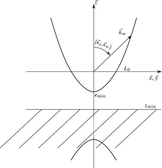
Then one shows easily from (A30) that x2 + y2 has a minimum for |$z_m = -z_0\frac{L/z_0}{1 + L^2/z_0^2} = -z_0 L/z_0 + \bigcirc \left(L^2/z_0^2\right)$| (|$\bigcirc \left(L^2/z_0^2\right) = \bigcirc \left(1\right)$|). Hence, |$z_m \simeq - \frac{A}{\alpha }\frac{\beta _\Vert }{\alpha }$| while |$z_\delta = \frac{A}{\beta _\Vert }$|. Using the fact that |$\alpha \lesssim \beta _\Vert$| one gets that zm ≲ zδ, which means zm is slightly under the bottom of the hyperboloid. Since x2 + z2 can be easily shown to be a growing function of z, its smallest value can only be zδ.
REFERENCES
APPENDIX A: Derivation of the general result
We show that domain of integration can be approximated by a hyperboloid of revolution. Then, we compute the integral Wk over this surface assuming that the distribution function of weak photons is given by a polynomial (e.g. Taylor expansion). A variety of notations and relations are used and we summarize them in Appendix B.
A1 Parametrization of L− by the three momentum of the weak photons
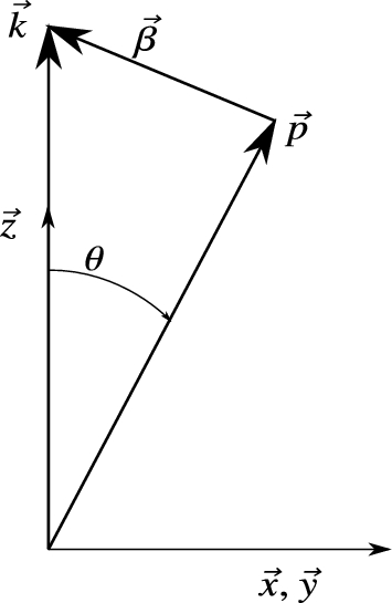
Coordinate system. In our approximation, |$\vec{k}$| is a quasi-symmetry axis.
