


Abstract
Calculation of the collisional rate coefficients with the most abundant species has been motivated by the desire to interpret observations of molecules in the interstellar medium. This paper will be concerned with rotational excitation of the phosphorus nitride (PN) molecule in its ground vibrational state by collisions with para-H2(j = 0). Ab intio potential energy surface for the PN–H2 van der Waals system, considering both molecules as rigid rotors, was computed via CCSD(T) method using the aug-cc-pVTZ basis sets, augmented by a bond functions placed at midway between the PN and H2 centres of mass. Cross-sections among the 40 first rotational levels of PN in collisions with para-H2(j = 0) were obtained using close coupling and coupled states calculations, for total energies up to 3000 cm− 1. Rate coefficients are presented for temperatures ranging from 5 to 300 K. A strong propensity favouring even Δj transitions is found. The comparison of the new PN–H2 rate coefficients with previously calculated PN–He rate coefficients shows that significant differences exist.
1 INTRODUCTION
Among the phosphorus-containing species, the phosphorus nitride (PN) is the first one detected in the interstellar medium. In 1987, two different groups have identified, in parallel investigations, interstellar PN by observation of its j = 2 → 1, j = 3 → 2, j = 5 → 4 and j = 6 → 5 rotational transitions toward Ori (KL), W51M and Sgr B2 stars (Turner & Bally 1987; Ziurys 1987). Since then, the PN molecule has been extensively observed by several groups using different techniques (Turner et al. 1990, 1992; Turner 1991; Schilke et al. 1997; Milam et al. 2008; De Beck et al. 2013; Fontani et al. 2016; Velilla Prieto et al. 2017). Having a large permanent dipole moment (μ = 2.75 D Wyse, Manson & Gordy 1972), the PN molecule has the advantage that its rotational lines are easily accessible to radio telescopes. Other phosphorus-bearing molecules (e.g. CP, HCP, PO, PH3) were detected in interstellar and circumstellar sources (Milam et al. 2008; De Beck et al. 2013; Agúndez et al. 2014).
Despite its fundamental role in biological systems (e.g. Pasek & Lauretta 2005), little is known about the phosphorus gas phase chemistry. The few theoretical works focused so far on the chemistry of interstellar phosphorus disagree in the prediction of the abundances of the main P-bearing molecules (see e.g. Charnley & Millar 1994; Maciá, Hernández & Oró 1997). Only the determination of the abundance of these molecules from observations can advance these models. The modelling of molecular emission from interstellar clouds requires the calculation of rate coefficients for excitation by collisions with H2, which is the most abundant species.
This paper focuses on rotational excitation rate coefficients of PN with para-H2 for temperatures ranging from 5 up to 300 K. The results were obtained using close-coupling method for transitions between lower rotational levels of PN and coupled-states approximation for higher levels. During the collision, we assumed that the para-H2 remains in its ground rotational state (j = 0), since at this range of temperature the probability to excite the j = 2 rotational level of H2 can be neglected (Kalugina, Kłos & Lique 2013; Lanza et al. 2014; Lique et al. 2015).
For this purpose, a new accurate ab initio potential energy surface (PES), averaged over the H2 orientations, was calculated using the coupled cluster approach. The new results are compared with those previously obtained for PN–He collisional system (Tobola et al. 2007). We then test the validity of the approximation for which collisional rate coefficients with para-H2 can be obtained from collisional rate coefficients with He by a simple multiplication by the square root of the ratio of the reduced masses of the collision systems (Green & Thaddeus 1974; Schöier et al. 2005).
The paper is structured as follows. Section 2 provides the details of the ab initio calculation of the potential energy surface. Scattering calculations are briefly described in Section 3. The discussion of our results is given in Section 4. Conclusions are given in Section 5.
2 THE PN − H2 POTENTIAL ENERGY SURFACE
In this work, we shall be concerned by rotational collisions of PN with para-H2 at low/moderate temperatures. During the PES calculations, both molecules were treated as rigid rotors. Recently, Faure et al. (2016) have shown for the CO–H2 system that state-averaged geometries give scattering results very close to full-dimensional calculations. Thus, we fixed the H2 molecular bond length at its average distance in the ground vibrational level: rHH = 1.449 Bohr, while PN was kept fixed at its experimental equilibrium geometry: rPN = 2.8173 Bohr (Huber & Herzberg 1979), which differs by less than 0.01 Bohr from the calculated value obtained by averaging over the ν = 0 vibrational wave function.
The Jacobi coordinate system corresponding to the collision process is displayed in Fig. 1. Relative to body-fixed system, the geometry of PN–H2 is described by three angles, θ, θ' and φ, and the intermolecular distance R. θ and θ' denote the polar angles of PN and H2 with respect to R, respectively, while φ is the azimuth angle of H2 molecule around R.
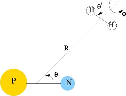
Jacobi coordinates describing the PN − H2 collisional system.
The collision occurs on the ground electronic state of the PN–H2 complex which is of 1A' symmetry. The adiabatic potential energy surfaces (PESs), function of R, θ, θ' and φ, were computed in the supermolecular approach by means of the highly correlated coupled cluster with single, double and perturbative triple excitations [CCSD(T)] method (Knowles, Hampel & Werner 1993, 2000). The ab initio calculations were done with the MOLPRO 2010 package (Werner et al. 2010). All atoms were described by the standard aug-cc-pVTZ (aVTZ) basis sets of Dunning (1989), augmented by the [3s3p2d2f1g] bond functions (BFs) optimized by Cybulski & Toczyłowski (1999) placed at mid-distance between the H2 centre of mass and the PN centre of mass.
For some characteristic geometries, we present in Table 1 a comparison of the interaction potential computed by our method CCSD(T)/aVTZ + BF with CCSD(T)-F12/aVTZ level of theory (Knizia, Adler & Werner 2009), recently used for many similar systems and proved to be accurate enough to describe van der Waals intermolecular interactions (see e.g. Bop et al. 2017; Bouhafs et al. 2017). A comparison with the standard CCSD(T), using basis sets aVTZ, aVQZ and a complete basis set (CBS) extrapolation, is also done. As one can see the inclusion of BFs increases significantly the rate of convergence of the interaction energy with respect to the basis size (this result also confirmed by Dubernet et al. 2015). The comparison also shows that the two methods (CCSD(T)/aVTZ + BF and CCSDT-F12/aVTZ) give similar results. Moreover, the difference between our CCSD(T)/aVTZ + BF data and the reference CCSD(T)/CBS is less than 5 per cent.
Interaction energies of PN − H2 system computed at different levels of theory for some characteristic geometries. All energies are in cm− 1 and distances in Bohr.
| Geometry | CCSD(T)/aVTZ | CCSD(T)/aVQZ | CCSD(T)/aVTZ + BF | CCSD(T)-F12/aVTZ | CCSD(T)/CBS |
|---|---|---|---|---|---|
| R = 8, θ = 0°, θ' = 0°, φ = 0° | −212.685 | −219.369 | −219.822 | −220.734 | −224.009 |
| R = 10, θ = 0°, θ' = 0°, φ = 0° | −94.146 | −94.575 | −94.688 | −94.254 | −95.212 |
| R = 14, θ = 0°, θ' = 0°, φ = 0° | −16.022 | −16.104 | −16.035 | −15.913 | −16.215 |
| R = 8, θ = 30°, θ' = 0°, φ = 0° | −172.719 | −177.391 | −178.328 | −178.853 | −180.7489 |
| R = 10, θ = 30°, θ' = 0°, φ = 0° | −69.778 | −70.291 | −70.354 | −70.160 | −70.817 |
| R = 14, θ = 30°, θ' = 0°, φ = 0° | −12.642 | −12.731 | −12.653 | −12.562 | −12.831 |
| R = 8, θ = 180°, θ' = 90°, φ = 90° | −61.150 | −67.054 | −67.573 | −67.596 | −70.747 |
| R = 10, θ = 180°, θ' = 90°, φ = 90° | −32.117 | −32.902 | −32.890 | −32.732 | −33.413 |
| R = 14, θ = 180°, θ' = 90°, φ = 90° | −5.781 | −5.893 | −5.749 | −5.784 | −5.972 |
| R = 8, θ = 90°, θ' = 90°, φ = 0° | −55.176 | −57.434 | −59.129 | −58.315 | −59.167 |
The values of the intermolecular distance R ranged from 5 to 30 Bohr. The grid included 13 values of θ ranging from 0° to 180° with a step of 15°. Three selected orientations, (θ' = 0°, φ = 0°), (θ' = 90°, φ = 0°) and (θ' = 90°, φ = 90°), of H2 molecule are calculated for each set of (R, θ). This resulted in a total of 1131 (R, θ, θ', φ) geometries calculated in Cs symmetry group for the PN–H2 system.
The geometry with θ = 0° and θ' = 0° corresponds to P − N⋅⋅⋅H − H collinear arrangement.
The one-dimensional PN–H2 potential energy curves, as a function of R, for θ = 0°, 90° and 180° are shown in Fig. 2 for the three H2 orientations. As can be seen, the potential has a relatively strong anisotropy due to H2 orientation. The most attractive interaction corresponds to P − N⋅⋅⋅H − H collinear geometry which is favoured by PN dipole and H2 quadrupole orientations. At linear configuration with θ = 180° and θ' = 0°, the attraction is weaker because of repulsive long-range electrostatic component of interaction which is due to an unfavourable PN dipole-H2 quadrupole orientation. For θ = 90°, the interaction potential, characterized by a relatively small electrostatic component of quadrupole–quadrupole origin, depends slightly on the orientation of H2 molecule.
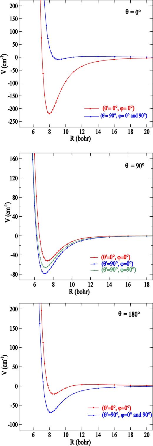
Potential curves of PN − H2, as a function of centre of mass separation, for different H2 orientations, (θ', φ) = (0°, 0°), (90°, 0°) and (90°, 90°), and for θ = 0° (upper panel), 90° (middle panel) and 180° (lower panel).
We approximate the average PES here by an equipoise averaging over the three PES's
Fig. 3 shows the contour plot for the averaged potential. The PN–H2 interaction energy minimum has a depth of − 72.65 cm− 1, located at about R = 7.55 Bohr and θ = 50.5°.
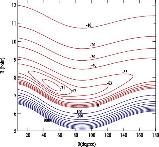
Contour plot of the PN − H2 interaction potential (in cm− 1), averaged over H2 orientations. The linear PN − H2 geometry corresponds to θ = 0.
It is interesting to compare our own PES for PN–H2 with the earlier PN − He PES of Tobola et al. (2007), calculated using similar theoretical approach. The two PESs have qualitatively the same behaviour, their well depths are comparable ( − 67.26 cm− 1 for PN–He), although the position of minimum of the PN–He PES is located in the linear He–PN configuration at R = 5.32 Bohr.
The calculated PES Vav is fitted with a least-squares routine to the analytical form given by equation (4) including expansion functions Pl up to lmax = 12. The quasi-symmetrical shape of PES with respect to θ↔π − θ (see Fig. 3) imposes a dominant contribution of the radial coefficients vl(R) with even l into the PES expansion (equation 4).
3 COLLISION DYNAMICS
The 2D PES Vav(R, θ) was used to compute cross-sections and rate coefficients for the rotational excitation due to collisions of PN(X1Σ) molecule with para-H2(j = 0). We do not take into account hyperfine excitation in PN because the component separation is not yet resolved by astrophysical observations (Cazzoli et al. 2006). By neglecting the rotational structure of the H2 molecule and the vibrational motion in PN molecule, the collisional problem reduces to rigid rotor colliding with a structureless projectile. The rotational energy levels for 31P14N were computed from the rotational constant B0 = 0.78649 cm− 1 (Wyse, Manson & Gordy 1972) and the centrifugal distortion constant D0 = 1.09 10− 6 cm− 1 (Huber & Herzberg 1979). Using such a reduced dimensional approach, we do expect an accuracy within 50 per cent for collisions with para-H2(j = 0) as already found by Lique et al. (2008) in the case of SiS − H2 collisions. At the opposite, using such an approach, it is not possible to estimate rate coefficients for collisions with H2 (j > 0) and full dimensional calculations will have to be performed in future studies to provide the astrophysical community with a full set of collisional data for PN molecules.
The close coupling (CC) formalism of Arthurs & Dalgarno (1960) is used to determine the cross-sections for transitions in PN molecule from rotational level j to rotational level j'. Unfortunatly, the accurate CC method is computationally too expensive for heavy molecule with small rotational constant. Accordingly, we used the coupled-states (CS) approximation (McGuire & Kouri 1974) to present cross-sections involving higher rotational levels j, j > 16. In the CC and CS approaches, the total inelastic cross-sections are obtained by including a sufficient total angular momentum partial waves J until convergence is reached (J = j + l, where l is the orbital angular momentum of the collision system).
The molscat code (Hutson & Green 1994) was used to solve the coupled scattering equations. Fully CC calculations between the first rotational levels j = 0 − 16 and CS approximation for transitions with j, 16 < j ≤ 39, were performed at values of the total energy ranging from 0 to 3000 cm− 1. The energy step sizes were chosen small enough to correctly describe the resonance structures of the inelastic cross-sections (specifically, 0.1 cm− 1 for total energies below 80 cm− 1). The variables which control the integration, such as Rmin, Rmax and STEPS (step size) were chosen to ensure convergence of the cross-sections over this range. For all energies the integration range extended from Rmin = 3 to Rmax = 40 Bohr. The rotational basis set employed in these calculations is extended to jmax = 28 and jmax = 54, respectively, for the CC and CS calculations. The maximum value of the total angular momentum quantum number J was fixed according to a convergence criterion of 1 per cent for the inelastic cross-sections.
4 RESULTS
4.1 Rotational cross-sections and rate coefficients
We illustrate in Fig. 4 the CC collisional excitation cross-sections as a function of collision energy for some typical Δj transitions in PN molecule. As may be seen, regardless the transition considered, the cross-sections show a dense resonance structure at low energies (Ec < 100 cm− 1). This relates to both shape resonances (open-channel resonances) and Feshbach resonances (closed-channel resonances) resulting from the decay of quasi-bound states of the PN⋅⋅⋅H2 (j = 0) complex, supported by the van der Waals well of the intermolecular potential (Taylor, Nazaroff & Golebieski 1966; Taylor 1970).
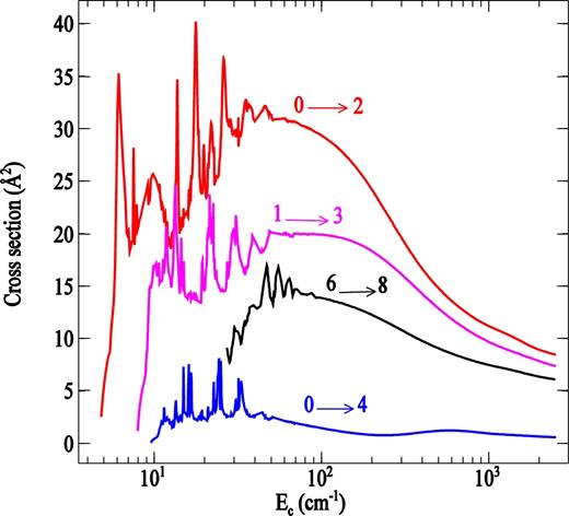
Rotational excitation cross-sections for selected transitions in PN molecule induced by para-H2(j = 0) as a function of the relative collision energy.
Fig. 5 displays rotational excitation cross-sections out the j = 0 level as functions of the final rotational quantum number. The cross-sections show a strong propensity favouring even Δj over odd Δj. This arises because the PN − H2(j = 0) interaction potential has nearly the symmetry of an atom-homonuclear diatomic system.
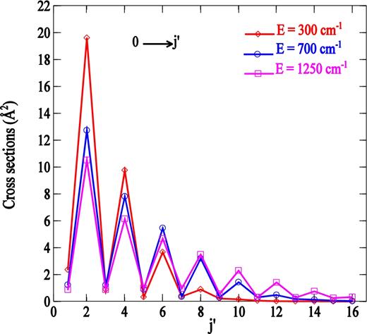
Cross-sections from the j = 0 level as a function of the final rotational quantum number at three selected total energies.
The coupled state approximation used in this work is known for its accurate results at high energies. This illustrated in Fig. 6, in which we compare the cross-sections predicted by both CS and CC approaches for the 0 → 2 transition. As expected, the CS cross-section differs significantly from that obtained using exact CC calculation at very low kinetic energy. This difference decreases rapidly with increasing energy. In Table 2, we also illustrate the degree of agreement between the two approaches at different total energy for transitions among low to higher rotational levels. As one can see beyond Ec > 350 cm− 1, the difference between CC and CS cross-sections is generally less than 10 per cent and not dependent on Δj transition even when j is large. Therefore, we can be confident in the accuracy of the CS calculations for transitions involving high rotational levels (j > 16) presented in this paper.
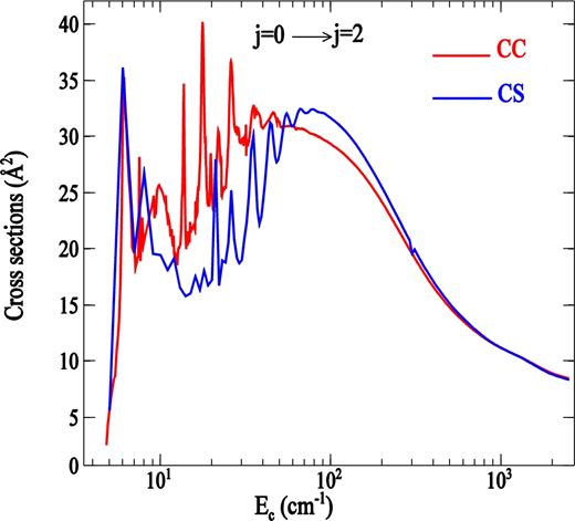
A comparison of CS and CC cross-sections for the j = 0 → j = 2 rotational transition in PN by collision with H2(j = 0) as a function of the collision energy.
Comparison between CC and CS cross-sections (in units of Å2) for different transitions at selected total energies.
| Transitions | E = 100 cm− 1 | E = 350 cm− 1 | E = 1000 cm− 1 | |||
|---|---|---|---|---|---|---|
| j → j' | CC | CS | CC | CS | CC | CS |
| σ1 → 0 | 1.86 | 2.74 | 0.70 | 0.84 | 0.33 | 0.36 |
| σ2 → 0 | 6.16 | 6.65 | 3.63 | 3.76 | 2.25 | 2.25 |
| σ2 → 1 | 2.69 | 3.92 | 1.10 | 1.30 | 0.65 | 0.70 |
| σ6 → 4 | 13.09 | 11.35 | 8.19 | 8.18 | 5.77 | 5.68 |
| σ10 → 8 | 33.70 | 37.74 | 9.44 | 9.02 | 6.03 | 5.90 |
| σ10 → 7 | 2.29 | 2.59 | 0.36 | 0.38 | 0.56 | 0.58 |
| σ10 → 6 | 4.56 | 3.43 | 3.03 | 2.94 | 2.63 | 2.53 |
| σ14 → 12 | – | – | 11.36 | 10.48 | 6.33 | 6.14 |
| σ14 → 11 | – | – | 0.37 | 0.42 | 0.58 | 0.60 |
| σ14 → 10 | – | – | 3.45 | 3.31 | 2.85 | 2.74 |
| σ14 → 9 | – | – | 0.17 | 0.18 | 0.37 | 0.39 |
| σ15 → 13 | – | – | 12.10 | 11.21 | 6.42 | 6.21 |
| σ15 → 12 | – | – | 0.38 | 0.44 | 0.58 | 0.60 |
| σ15 → 11 | – | – | 3.58 | 3.44 | 2.90 | 2.79 |
| σ16 → 14 | – | – | 13.00 | 12.28 | 6.51 | 6.28 |
| σ16 → 13 | – | – | 0.40 | 0.47 | 0.58 | 0.61 |
| σ16 → 12 | – | – | 3.72 | 3.62 | 2.96 | 2.86 |
| σ16 → 11 | – | – | 0.21 | 0.23 | 0.37 | 0.39 |
| σ18 → 16 | – | – | 16.80 | 17.26 | 6.72 | 6.45 |
| σ18 → 17 | – | – | 2.21 | 1.64 | 1.00 | 1.07 |
Rate coefficients which derive from the above cross-sections (equation 6) are displayed in Fig. 7 as a function of temperature for some transitions. As expected, the same propensity rules favouring even Δj transitions are observed. The rate coefficients for |Δj | = 2 transitions were about a factor of 3 larger than those for |Δj | = 1, especially at high temperatures. The complete sets of de-excitation rate coefficients will be made available online from the BASECOL1 website (Dubennet et al. 2013).
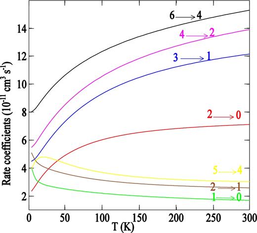
Temperature dependence of the rate coefficients for the rotational de-excitation of PN by para-H2(j = 0) for Δj = − 1 and Δj = − 2 transitions.
4.2 Comparison with PN − He rate coefficients
It is interesting to compare our new rate coefficients for rotational excitation of PN by para-H2(j = 0) with rate coefficients for excitation of PN by He calculated previously using the same methodology (Tobola et al. 2007). It is generally assumed that the excitation rate coefficients for para-H2(j = 0) were deduced from the He ones using a simple scaling factor, which accounts for the difference in reduced masses of He and H2 (Schöier et al. 2005). For PN molecule, this factor is|${\rm{\ }}{( {{\mu _{{\rm{PN}} - {{\rm{H}}_2}}}/{\mu _{{\rm{PN}} - {\rm{He}}}}} )^{1/2}} = \ 1.38$|. To assess the validity of this approximation, we report in Fig. 8 the PN − H2(j = 0) de-excitation rate coefficients as a function of the PN − He ones for Δj = j' − j = − 1, − 2, − 3, ⋅⋅⋅ transitions with j' ≤ 12 at a temperature of 100 K. The ratio of the two rate coefficients for Δj = − 1 is close to 1.38 but begins to deviate when Δj increases and reaches a factor 1/10 for large Δj. The reason for this difference is to be found in interaction potentials. A comparison of the two different sets of coefficients of the potential expansion (see Fig. 9) shows a comparable importance of the v1 anisotropy terms of the two PES (equation 4); on the other hand, the difference between vl > 1 anisotropy terms is relatively large and varies with the distance. This may explain why Δj = 1 agree with this scaling procedure and why the others do not. Thus, we can conclude that the multiplication of rate coefficients for PN − He collision by a scaling factor of 1.38 to estimate the H2 rate coefficients is unreliable. The result confirms previous results obtained for other molecules like NH2 (Bouhafs et al. 2017), C2H (Najar et al. 2014) or C2 (Najar et al. 2009).
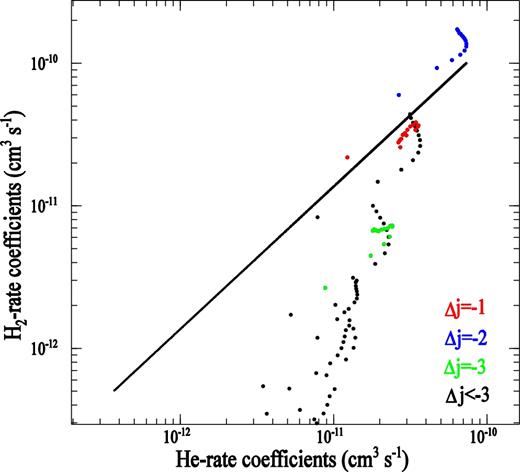
PN − H2 (j = 0) rate coefficients as a function of the PN − He rate coefficients for j' → j de-excitations with j' ≤ 12 at a temperature of 100 K. The solid line refers to a ratio of 1.38.
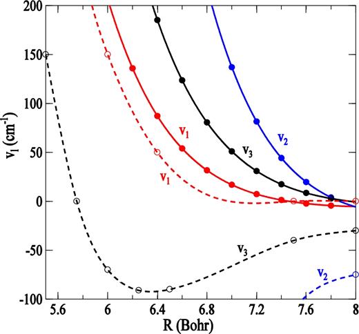
Plot of first anisotropic terms of radial Legendre expansion coefficients (l = 1, 2, 3). Solid curves for PN − H2 system; dashed curves for PN − He system (Tobola et al. 2007).
For astrophysical applications, as shown by Lique et al. (2015) for similar system, the new rate coefficients can lead to reconsideration of the estimate of PN abundance in molecular clouds.
5 SUMMARY AND CONCLUSION
We have used a new PN − H2 potential energy surface, averaged over three orientations of the H2 molecule, to study rotationally inelastic collisions between PN and para-H2(j = 0). Rate coefficients were determined for temperatures 5K < T < 300 K. Propensity rules favouring even Δj over odd Δj were found. As shown by Wernli et al. (2007) in HC3N − H2 collisions, this propensity can amplify population inversion in the rotational levels of interstellar PN.
A comparison of the present PN-para-H2 rate coefficients with scaled PN − He rate coefficients reveals discrepancies especially for large Δj, which may indicate significant differences in anisotropic parts of the two potentials.
In any case, these new rate coefficients will be useful for the interpretation of PN observations.
REFERENCES
