


Abstract
The Calar Alto Legacy Integral Field Area (CALIFA) survey, a pioneer in integral field spectroscopy legacy projects, has fostered many studies exploring the information encoded on the spatially resolved data on gaseous and stellar features in the optical range of galaxies. We describe a value-added catalogue of stellar population properties for CALIFA galaxies analysed with the spectral synthesis code starlight and processed with the pycasso platform. Our public database (http://pycasso.ufsc.br/, mirror at http://pycasso.iaa.es/) comprises 445 galaxies from the CALIFA Data Release 3 with COMBO data. The catalogue provides maps for the stellar mass surface density, mean stellar ages and metallicities, stellar dust attenuation, star formation rates, and kinematics. Example applications both for individual galaxies and for statistical studies are presented to illustrate the power of this data set. We revisit and update a few of our own results on mass density radial profiles and on the local mass–metallicity relation. We also show how to employ the catalogue for new investigations, and show a pseudo Schmidt–Kennicutt relation entirely made with information extracted from the stellar continuum. Combinations to other databases are also illustrated. Among other results, we find a very good agreement between star formation rate surface densities derived from the stellar continuum and the H α emission. This public catalogue joins the scientific community’s effort towards transparency and reproducibility, and will be useful for researchers focusing on (or complementing their studies with) stellar properties of CALIFA galaxies.
1 INTRODUCTION
The modus operandi of extragalactic astrophysics was transformed by large spectroscopic surveys, such as the 2dF Galaxy Redshift Survey (Colless et al. 2001) and the Sloan Digital Sky Survey (SDSS; York et al. 2000). Instead of relying on a few dozen galaxies, now hundreds of thousands are routinely summoned to address a wide variety of astrophysical questions. The combination of large surveys with stellar population libraries with good spectral resolution (e.g. Bruzual & Charlot 2003) was the cornerstone for the uprise of several spectral synthesis codes, such as our own code starlight (Cid Fernandes et al. 2005), and those by other groups: moped (Panter, Heavens & Jimenez 2003), stecmap/steckmap (Ocvirk et al. 2006a,b), vespa (Tojeiro et al. 2007) and ulyss (Koleva et al. 2008).
One example of the statistical power of applying starlight to a million SDSS galaxy spectra was revealing a huge and forgotten population of retired galaxies ionized by hot low-mass evolved stars (HOLMES), whose spectra are confounded with those of low-ionization nuclear emission regions (Stasińska et al. 2008; Cid Fernandes et al. 2010, 2011). This population completely changes the census of galaxies in the local Universe (Stasińska et al. 2015). Other examples include studies of the stellar mass–metallicity relation (Vale Asari et al. 2009), the chemical evolution and the star formation (SF) history of local galaxies (Asari et al. 2007; Cid Fernandes et al. 2007), how to distinguish active galactic nucleus (AGN) hosts (Stasińska et al. 2006), the bimodality of galaxies and the downsizing (Mateus et al. 2006), and the dependence of galaxy properties on the environment (Mateus et al. 2007). More importantly in the context of this paper, the data and tools behind these studies were made publicly available, fostering independent research. Since having published our value-added starlight-SDSS catalogue (Cid Fernandes et al. 2009) in a public database (http://starlight.ufsc.br), studies like Bian et al. (2007), Liang et al. (2007), Peeples, Pogge & Stanek (2009), Riffel et al. (2009), Lara-López et al. (2009a), Lara-López et al. (2009b), Lara-López et al. (2010) and Andrews & Martini (2013) have used our code and database.
These past few years have witnessed the surge of integral field spectroscopy (IFS) observations. While SDSS obtained one spectrum per galaxy, IFS surveys commit to spectrally map galaxies pixel by pixel. The Calar Alto Legacy Integral Field Survey Area survey (CALIFA; Sánchez et al. 2012) was a pioneer wide-field IFS survey of nearby galaxies. Its Data Release 3 (DR3; Sánchez et al. 2016c) contains 445 galaxy COMBO data cubes covering 3700–7500 Å and in the redshift range 0.005 < z < 0.03. The COMBO cubes have a resolution of 850, approximately FWHM = 6 Å at λ = 5000 Å. The spatial sampling is 1 arcsec, with a point spread function (PSF) given by a Moffat profile with FWHM = 2.5 arcsec and β = 2. CALIFA provides a statistically significant sample that is complete in the magnitude range −19.0 < Mr < −23.1 and stellar masses1 between 109.7 and 1011.4 M⊙ (Walcher et al. 2014). In addition to its clear selection criteria, another characteristic that sets CALIFA apart is its spatial coverage (>2 half-light radius), which maps galaxies farther in their outskirts than other ongoing surveys such as SAMI (Croom et al. 2012) and MaNGA (Bundy et al. 2015).
We have analysed the CALIFA data cubes with our spectral synthesis code starlight and the python CALIFA starlight Synthesis Organiser (pycasso) platform, as described in Cid Fernandes et al. (2013, 2014).This formed the basis of a series of studies about the spatially resolved stellar population properties, where we have obtained the following:
Evolutionary curves of the cumulative mass function, tracing the mass assembly history of ∼100 galaxies as a function of the radial distance (Pérez et al. 2013). The results suggest that galaxies grow inside-out, as confirmed by García-Benito et al. (in preparation) for a seven times larger sample.
2D maps and spatially resolved information of the stellar population properties used to retrieve the local relations between the following: (a) stellar mass surface density, Σ⋆, and luminosity-weighted stellar ages, 〈log t〉L (González Delgado et al. 2014a); (b) mass-weighted stellar metallicity, 〈log Z〉M, and Σ⋆ (González Delgado et al. 2014b); (c) the intensity of the star formation rate, ΣSFR, defined in this work as the star formation rate (SFR) surface density, and Σ⋆ (González Delgado et al. 2016). These relations indicate that local processes are relevant to regulate the SF and chemical enrichment in the disc of spirals. For spheroids, on the other hand, the stellar mass, M⋆, regulates these processes.
Radial profiles of stellar extinction, AV, Σ⋆, 〈log t〉L, 〈log Z〉M, and their radial gradients also confirm that more massive galaxies are more compact, older, metal rich and less reddened by dust. These trends are preserved spatially as a function of the radial distance to the nucleus. Deviations from these relations seem to be correlated with Hubble type: earlier types are more compact, older and more metal rich for a given M⋆, which evidences that the shutdown of the SF is related to galaxy morphology (González Delgado et al. 2015a). The negative radial gradients of 〈log t〉L and 〈log Z〉M also confirm that galaxies grow inside-out.
The radial profiles of ΣSFR and the small dispersion between the profiles of late-type spirals (Sbc, Sc, Sd) confirm that the main sequence of the star-forming galaxies is a sequence with nearly constant ΣSFR (González Delgado et al. 2016). Furthermore, the radial profiles of local and recent specific star formation rate (sSFR) depend on Hubble type (increasing as one goes from early to late types) and increase radially outwards. This behaviour suggests that galaxies are quenched inside-out, and that this process is faster in the central bulge-dominated parts than in the discs (González Delgado et al. 2016).
From the 2D (R × t) map of the galaxy SFH, we retrieve the spatially resolved time evolution information of the SFR, its intensity (ΣSFR) and sSFR. We find that galaxies form very fast independently of their stellar mass, with the peak of SF at high redshift (z > 2), and that subsequent SF is driven by M⋆ and morphology, with less massive and late-type spirals showing more prolonged periods of SF (González Delgado et al. 2017).
From the comparison of the spatially resolved and the integrated spectra analyses, we find that the stellar population properties are well represented by their values at one half-light radius (HLR; González Delgado et al. 2014a).
Detailed studies of a small sample of galaxies are very well served by the CALIFA survey and our analysis. For example, the analysis of the spatially resolved SFH of mergers (Cortijo-Ferrero et al. 2017a; Cortijo-Ferrero et al. 2017b,c) in comparison with ‘non-interacting’ spiral galaxies allows us to estimate the effect of the merger phase in the enhancement of the SF and their spatial extent, as well as to trace the merger epochs.
By extending starlight to combine CALIFA optical spectra and GALEX (Martin et al. 2005) UV photometric data, the uncertainties in stellar properties become smaller (López Fernández et al. 2016). Also, young stellar populations are better constrained, especially for low-mass late-type galaxies, where there is a significant <300 Myr population.
The well-defined selection function of the survey allows for reliable volume corrections (Walcher et al. 2014). Combining these with our homogeneous analysis led to an estimation of the SFR density of the Local Universe of 0.0105 ± 0.0008 M⊙ yr−1 Mpc−3, in agreement with independent estimates (González Delgado et al. 2016; see also López Fernández et al., in preparation).
We release the data used in those papers in a public value-added catalogue (http://pycasso.ufsc.br/, mirror at http://pycasso.iaa.es/). The data were updated to the latest CALIFA release (DR3) and reduction pipeline (v2.2). Stellar population models used in the starlight fits were also updated. These modifications have only minor effects with respect to the results reported in the studies mentioned above. Still, when exemplifying the use of this new database we will take the opportunity to revisit and update some of our previous results.
In addition to embracing the ethos of open science data and tools to encourage reproducible results, our CALIFA-starlight value-added catalogue can be used for many different purposes. We list a few of those, based on the impact of our former SDSS-starlight public database: (a) Stellar population data may be used to complement studies focused on nebular properties. (b) Our catalogue can be used to investigate the host galaxy of transient sources. For instance, if there is a supernova explosion in a CALIFA galaxy 10 yr from now, interested researchers need simply to look up the corresponding spaxel in our catalogue (Stanishev et al. 2012; Galbany et al. 2014). (c) Finally, other groups might be interested in the stellar population themselves, using our database with a different perspective from our group.
This paper is organized as follows. Section 2 describes the CALIFA observations and the sample selection. In Section 3, we discuss how CALIFA galaxies are analysed with starlight, our spectral synthesis code and pycasso, a tool to organize the synthesis results for IFS data. Section 4 describes the physical and quality control maps available in our value-added catalogue, as well as details on how to access the data. Section 5 shows a few example usages for the catalogue. Some comparisons to data from other sources are presented in Section 6. Our concluding remarks follow in Section 7.
2 OBSERVATIONS AND SAMPLE
The survey data were collected using the Potsdam Multi-Aperture Spectrophotometer (Roth et al. 2005) in PPak mode (Kelz et al. 2006). PPak is a bundle of 382 fibres, each one having 2.7 arcsec of diameter. It covers a field of view (FoV) of 74 arcsec × 64 arcsec, with a filling factor of ∼60 per cent.
Observations for CALIFA were obtained in two different spectral settings using the V500 and V1200 gratings. The V500 grating has a spectral resolution of ∼ 6 Å (FWHM), with a wavelength coverage from 3745 to 7300 Å, while the V1200 has a higher spectral resolution of ∼2.3 Å, covering the 3650–4840 Å range. However, vignetting on the CCD corners reduces the useful wavelength range in some regions of the FoV. The vignetting can be reduced by combining observations using V500 and V1200 gratings. These are called COMBO cubes. A dithering scheme using three observations is used to fill the whole FoV. More information on the observational strategy, effects of vignetting, the reduction pipeline and data quality can be found in Sánchez et al. (2012) and Sánchez et al. (2016c).
The sample is formed by 445 galaxies of the final CALIFA data release DR3 (Sánchez et al. 2016c) that were observed with both V500 and V1200, and have COMBO cubes. This sample includes 395 galaxies from the main sample, the remaining galaxies are from the extended CALIFA sample. The main sample is a statistically significant subset of the mother sample, which in turn was drawn from the SDSS DR7 (Abazajian et al. 2009). It consists of a representative sample of galaxies of the local Universe at the redshift range 0.005 < z < 0.03, with magnitudes (−24 < Mr < −17) and colours (u − r < 5) that cover all the colour–magnitude diagram (CMD). The galaxies were selected by their apparent size with an angular isophotal diameter 45 arcsec < isoAr < 80 arcsec to fill the FoV of PPaK. A full description of the mother sample is in Walcher et al. (2014). The extended CALIFA sample comes from a heterogeneous set of galaxies observed in different ancillary science projects that are fully described in Sánchez et al. (2016c).
The galaxies from the main and the extended samples were morphologically classified by members of the collaboration through a visual inspection of the SDSS r-band images.2 Fig. 1(a) shows the location of the main sample galaxies in the CMD, compared to the mother sample. The distribution by morphological type, again for both samples, is shown in Fig. 1(b).
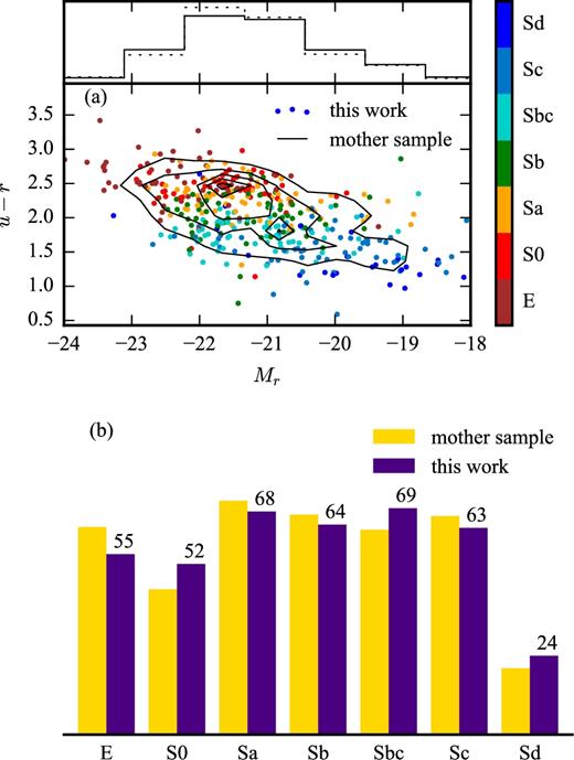
Panel (a): Color–magnitude diagram (CMD) of the sample, using photometric magnitudes from SDSS DR7. The black contours show the density of galaxies in the mother sample. The dots, coloured by morphological type, show the 395 galaxies with COMBO cubes from the main sample. Above the CMD is the Mr histogram of both the mother sample, as a black line, and the 395 galaxy sample, as a dotted line. Panel (b): histogram of morphological types of the mother sample (red bars) and the 395 galaxy sample (blue bars). The histograms are normalized for comparison between the two distributions. The number of galaxies in each type for the 395 galaxies from the main sample is printed above the blue bars.
3 METHOD OF ANALYSIS
We use a full spectral approach to the stellar population synthesis, using starlight. The cubes pass through a series of pre-processing steps, meant to extract good quality data for the analysis. These are part of the qbick pipeline, described in detail in the section 3.2 of Cid Fernandes et al. (2013). The main steps are briefly discussed below.
3.1 Pre-processing
The first step is to mask all spaxels containing light from spurious sources. This includes foreground stars and other galaxies in the FoV. The outer spaxels that have S/N < 3 are also masked.
The cubes are then segmented in Voronoi zones, as implemented by Cappellari & Copin (2003). We use, as input, signal and noise images from the 5635 ± 45 Å spectral range (the same that is used for spectra normalization, as discussed below). Some modifications were done on the co-added error estimation to account for spatial covariance, as described in the appendix of García-Benito et al. (2015). The target S/N was 20, which lead to most zones inside 1 HLR consisting of a single spaxel.
3.2 Spectral synthesis
After the pre-processing steps the resulting spectra are fitted using starlight (Cid Fernandes et al. 2005). We fit the λ = 3700–6850 Å rest-frame stellar continuum, masking spectral windows around emission lines ([O ii]λ3726/3729, H γ, H β, [O iii]λ5007, He iλ5876, [O i]λ6300, H α, [N ii]λ6584, [S ii]λ6716/6731). We further mask the Na i doublet at λ = 5890 Å because of possible absorption in the neutral interstellar medium.
The fits decompose the observed spectra in a base built from single stellar populations (SSP). Model SSP spectra are a central ingredient in our analysis, which allow us to link the results of the spectral decomposition to physical properties of the stellar populations. Our previous analysis of CALIFA data (reviewed in Section 1) explored different sets of SSP spectra, varying the number of components, the range in metallicity, the specific ages of the SSP, initial mass function (IMF) and stellar evolution. The fits presented here were obtained using two sets of bases, labelled as GMe and CBe, that have been extensively tested and compared (González Delgado et al. 2015b,c; González Delgado et al. 2016). These bases are similar to bases GM and CB of Cid Fernandes et al. (2014), but extended in terms of the metallicity coverage.
Base GMe is a combination of 235 SSP spectra from Vazdekis et al. (2010), for populations older than 63 Myr, and González Delgado et al. (2005) models, for younger ages. The evolutionary tracks are those from Girardi et al. (2000), except for the youngest ages (1 and 3 Myr), which are based on the Geneva tracks (Schaller et al. 1992; Charbonnel et al. 1993; Schaerer et al. 1993a,b). The metallicity covers the seven bins provided by Vazdekis et al. (2010): log Z/Z⊙ = −2.3, −1.7, −1.3, −0.7, −0.4, 0, +0.22, but for SSP younger than 63 Myr, Z includes only the four largest metallicities. The chosen IMF is Salpeter.
Base CBe is a combination of 246 SSP spectra provided by Charlot & Bruzual (2007, private communication,3) covering 41 ages from 0.001 to 14 Gyr, with six metallicities: log Z/Z⊙ = −2.3, −1.7, −0.7, −0.4, 0, +0.4. The IMF is that from Chabrier (2003). These SSP are an update of the Bruzual & Charlot (2003) models, where STELIB (Le Borgne et al. 2003) is replaced by the MILES (Sánchez-Blázquez et al. 2006) and GRANADA (Martins et al. 2005) spectral libraries. The stellar tracks are those known as ‘Padova 1994’ (Alongi et al. 1993; Bressan et al. 1993; Fagotto et al. 1994a,b,c; Girardi et al. 1996).
Other important issues in our methodology are as follows: (a) dust effects are also modelled in the spectral fits as a foreground screen with a Cardelli, Clayton & Mathis (1989) reddening law with RV = 3.1; (b) kinematics effects are also taken into account, assuming a Gaussian line-of-sight velocity distribution. Both spectral bases are smoothed to 6 Å FWHM effective resolution prior to the fits. This is because the kinematical filter implemented in starlight operates in velocity-space, whereas both CALIFA and the SSP spectra have a constant resolution in λ-space. This way the velocity dispersion obtained by starlight is not contaminated by the spectral resolution mismatch.
3.3 PyCASSO
starlight was developed to work with individual spectra. The pycasso platform was developed to organize its output into spatially resolved data.
The output produced by starlight is quite large, and it takes a little effort to transform some of the values into familiar physical measurements. pycasso takes care of these computations and provides convenient functions that allow us to deal directly with the physical maps. This made the exploration of the data a lot easier, yielding the various results discussed in Section 1. These physical maps (and some diagnostic ones) are published in this database, and are described in the following section.
4 DESCRIPTION OF THE CATALOGUE
The catalogue is comprised of fits files containing images for a suite of physical properties of each galaxy of the sample. The files also contain quality control and fit diagnostic maps. A fits table with properties derived for the integrated spectra of the galaxies is also available. We present these data products below.
4.1 Map data format
Maps are distributed in multi-extension binary fits files, containing several HDUs. The HDUs consist of a header and an image extension. The headers are all the same for all HDUs, except for the first (primary), which contains additional cards. In particular, CALIFA_ID and NED_NAME are present for object identification. BASE informs which SSP base was used in the fit; it may be either gsd6e (the GMe base) or zca6e (the CBe base). Also worth mentioning is the luminosity distance used when calculating masses, stored in the card DL_MPC, in units of Mpc. All headers also contain celestial WCS extracted from the original COMBO cubes.
For a given galaxy, the maps are images with the same dimensions. The exact dimensions will change for each galaxy; they are the same as the raw cubes from DR3. Except for badpix and zones, which are integers, all data are stored as 64-bit floating point numbers. If a pixel is considered ‘bad’ (see Section 4.5.1), its value in all maps is set to zero.4 The 12 first HDUs, listed in Table 1, contain maps with physical results from starlight. The remaining 7 HDUs contain data and fit diagnostic maps. The content of these maps are explored in detail in Sections 4.4 and 4.5.
Physical quantities and diagnostic maps present in the galaxy cubes.
| HDU | Quantity | Units | Extension name | Description |
|---|---|---|---|---|
| 0 | Σ⋆ | M⊙ pc−2 | sigma_star | Stellar mass surface density. Mass that is currently trapped inside stars. |
| 1 | |$\Sigma ^\prime _\star$| | M⊙ pc−2 | sigma_star_ini | Initial stellar mass surface density. Mass ever formed into stars. |
| 2 | |$\mathcal {L}_{5635{A\!\!\!\!\!^{^\circ}}}$| | L⊙ Å−1 pc−2 | L_5635 | Luminosity surface density in the 5635 Å normalization window. |
| 3 | 〈log t〉L | log yr | log_age_flux | Mean log of stellar age, in years, weighted by luminosity. |
| 4 | 〈log t〉M | log yr | log_age_mass | Mean log of stellar age, in years, weighted by mass. |
| 5 | 〈log Z〉L | log Z⊙ | log_Z_flux | Mean log of stellar metallicity, in solar units, weighted by luminosity. |
| 6 | 〈log Z〉M | log Z⊙ | log_Z_mass | Mean log of stellar metallicity, in solar units, weighted by mass. |
| 7 | ΣSFR | M⊙ Gyr−1 pc−2 | sigma_sfr | Mean star formation rate surface density in the last 32 Myr. |
| 8 | xY | – | x_young | Luminosity fraction of stellar populations younger than 32 Myr. |
| 9 | τV | – | tau_V | Attenuation coefficient for a dust screen model. |
| 10 | v⋆ | km s−1 | v_0 | Line-of-sight velocity. |
| 11 | σ⋆ | km s−1 | v_d | Line-of-sight velocity dispersion. |
| 12 | |$\overline{\Delta }$| | per cent | adev | Mean model deviation. |
| 13 | Nλ, clip/Nλ | per cent | nl_clip | Fraction of the wavelengths clipped by the fitting algorithm. |
| 14 | |$\chi ^2/N_\lambda ^\mathrm{eff}$| | – | chi2 | Fit statistic. |
| 15 | Bad pixels | – | badpix | Masked pixels. |
| 16 | Zones | – | zones | Voronoi segmentation zones. |
| 17 | S/N | – | sn | Signal-to-noise ratio in individual pixels. |
| 18 | S/N (zones) | – | sn_zone | Signal-to-noise ratio in zones. |
4.2 Integrated spectra table data format
We also fit the integrated spectra of the galaxies, summing the flux from all non-masked spaxels. The data are stored in a binary fits table, with columns described in Table 2. The data are stored as 64-bit floating point numbers, except for califaID, which is integer, and NED_name and base, which are text strings. The quantities in this table are the same ones provided as maps. Note, however, that the extensive quantities in this table (luminosity, stellar masses and SFR) are not surface densities.
Global properties of galaxies using integrated spectra.
| Quantity | Units | Column | Description |
|---|---|---|---|
| CALIFA ID | – | califaID | CALIFA galaxy ID. |
| Object name | – | NED_name | Object name. |
| Luminosity distance | Mpc | DL_Mpc | Luminosity distance used when calculating stellar masses. |
| SSP base | – | base | Base used in the fit. |
| M⋆ | M⊙ | M_star | Stellar mass currently trapped inside stars. |
| |$M^\prime _\star$| | M⊙ | M_star_ini | Total mass ever formed into stars. |
| L5635Å | L⊙ Å−1 | L_5635 | Luminosity in the 5635 Å normalization window. |
| 〈log t〉L | log yr | log_age_flux | Mean log of stellar age, in years, weighted by luminosity. |
| 〈log t〉M | log yr | log_age_mass | Mean log of stellar age, in years, weighted by mass. |
| 〈log Z〉L | log Z⊙ | log_Z_flux | Mean log of stellar metallicity, in solar units, weighted by luminosity. |
| 〈log Z〉M | log Z⊙ | log_Z_mass | Mean log of stellar metallicity, in solar units, weighted by mass. |
| SFR | M⊙ Gyr−1 | sfr | Mean star formation rate in the last 32 Myr. |
| xY | – | x_young | Luminosity fraction of stellar populations younger than 32 Myr. |
| τV | – | tau_V | Attenuation coefficient for a dust screen model. |
| v⋆ | km s−1 | v_0 | Line-of-sight velocity. |
| σ⋆ | km s−1 | v_d | Line-of-sight velocity dispersion. |
| |$\chi ^2/N_\lambda ^\mathrm{eff}$| | – | chi2 | Fit statistic. |
| |$\overline{\Delta }$| | per cent | adev | Mean model deviation. |
| Nλ,clip/Nλ | per cent | nl_clip | Fraction of the wavelengths clipped by the fitting algorithm. |
4.3 Data access
The data are publicly available at the PyCASSO web site (http://pycasso.ufsc.br/, mirror at http://pycasso.iaa.es/). The galaxies are listed with a colour SDSS image stamp for reference. There are some preview plots available for each galaxy, in the same fashion as Fig. 2. fits files with the maps are also available for download, with names following the convention: KNNNN_base.fits. The file names always start with K, and NNNN is the CALIFA ID, padded with zeros up to four digits. The suffix base indicates the base used in the fit, which can be gsd6e, for base GMe, or zca6e, for base CBe. For example, the galaxy shown in Fig. 2, fitted using GMe, is stored as K0140_gsd6e.fits. Tables with integrated data fitted with both bases are also available for download, with the same suffixes indicating which base.
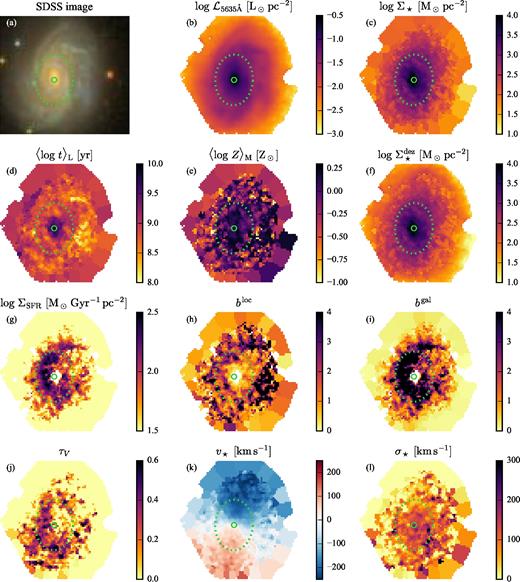
Maps with physical properties of CALIFA 0140. A dotted ellipse marks the 1 HLR area, and a small circle marks the galaxy centre. See Table 1 for a brief description of each map.
There is also a form for selecting galaxies based on some of their characteristics. These may be observational (Hubble type, SDSS magnitudes, etc.) or physical quantities obtained on integrated spectra (stellar mass, mean stellar age, τV, etc.). Given that the data set is small (445 galaxies × 2 bases), a simple search form suffices.
The observed data used as input for this work are available at the CALIFA web site (http://califa.caha.es/DR3/).
4.4 Description of the physical maps
To facilitate the description and illustrate the information content of the catalogue, Fig. 2 shows the maps for a sample galaxy, CALIFA 0140 (NGC 1667). The SDSS image5 of this galaxy is shown in panel (a). This is a low inclination Sbc galaxy, with a small bar. It has an HLR6 (computed in the 5635 ± 45 Å normalization band) of 15.1 arcsec, with an ellipticity of ε = 0.26 and position angle of 177°.
In what follows we describe each of the maps available, as well as ways of processing them to improve the results or express them in other forms to highlight certain aspects of the data.
4.4.1 Luminosity and stellar mass surface densities
The luminosity surface density (|$\mathcal {L}_{5635\,{A\!\!\!\!\!^{^\circ}}}$|, Fig. 2b) associated with each spaxel is calculated directly from the observed spectra using the median flux in the spectral window of 5635 ± 45 Å. The map has units of L⊙ Å−1 pc−2. The bulge and spiral arms are clearly visible in the image.
The stellar mass surface density (Σ⋆, Fig. 2c) is calculated using the masses derived from starlight, and are provided in units of M⊙ pc−2. This mass has been corrected for mass that returned to the interstellar medium during stellar evolution, so it reflects the mass currently in stars. The uncorrected mass, i.e. the total mass ever turned into stars, |$\Sigma ^\prime _\star$|, is also included in the database.
The morphological structures are still visible in the Σ⋆ map. None the less, an artefact is evident in the Σ⋆ map: the outer parts of the galaxy are broken in flat patches. This happens because we combine the lower S/N spaxels that are spatially close into Voronoi zones before running starlight. This behaviour occurs in all maps that are products of the synthesis. Only |$\mathcal {L}_{5635\,{A\!\!\!\!\!^{^\circ}}}$|, which comes directly from the spectra, is presented as a full resolution image.
4.4.2 Dezonification
Before proceeding with the description of the catalogue maps, it is useful to present a simple data processing to smooth over the spatial effects of the Voronoi zones used in the spectral fitting, as those seen in the image of Σ⋆ (Fig. 2c). This procedure was first introduced by Cid Fernandes et al. (2013) to smooth extensive properties, and is generalized below.
By design, the total mass of the zones does not change, we only redistribute the mass among their pixels. Fig. 2(f) shows an example of dezonification using α = 1.4. This value was found by fitting Σ⋆ as a function of |$\mathcal {L}_{5635\,{A\!\!\!\!\!^{^\circ}}}$| for our example galaxy, as seen in Fig. 3(a). In Fig. 3(b), we show radial profiles of Σ⋆, the original (dots and black line) and dezonified versions with various values of α. Inwards of ∼1.7 HLR, the curves are identical, because zones there actually correspond to single spaxels (N = 1). At larger radii, the α = 1.4 line (in green) seems to better represent the cloud of dots for this galaxy, while without dezonification (black line) the profile becomes artificially flatter. Note that the value for α was calculated for this galaxy only. Other values may be needed for other galaxies, and can be straightforwardly obtained with the data provided in the catalogue. The same overall procedure can be applied to any property that is extensive, that is, scales with the size of the system (for instance, |$\Sigma ^\prime _\star$| and ΣSFR). Intensive properties, like age and metallicity, are inherently ‘undezonifiable’.
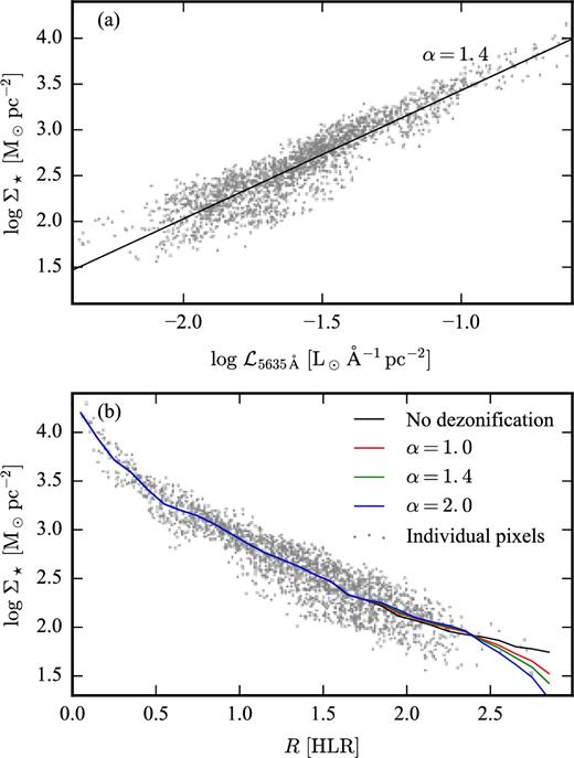
Dezonification (see Section 4.4.1) of the mass surface density for CALIFA 0140. Panel (a): mass–luminosity plot to derive the α parameter used in equation (1). The black line is the linear fit to the data (grey dots). Panel (b): radial profile of the mass surface density. The dots are the mean mass surface density in each zone. The black line is the mean radial profile without dezonification, while the coloured lines are the profiles with dezonification for different α values. The value used in this work is α = 1.4 (green).
4.4.3 Mean stellar age and metallicity
The luminosity-weighted mean stellar age (equation 3) and mass-weighted mean stellar metallicity (equation 6) are shown in panels (d) and (e) of Fig. 2. Most of the works on stellar population use these two definitions. Stellar metallicity is directly related to the mass, which justifies this choice. On the other hand, the mean age spans a larger dynamical range weighting by light, which helps better mapping younger populations. A spiral pattern is present in both maps, following the spiral seen in luminosity. Negative gradients are present in both age and metallicity. These become more evident with a little processing of the data, as seen in Section 5.1.
These are all intensive quantities, independent of the size of the system. Thus, unlike Σ⋆ and ΣSFR, they are intrinsically not dezonifiable.
4.4.4 Star formation rate surface density
Fig. 2(g) shows the map of the mean recent SFR surface density7 (ΣSFR), obtained by adding the mass turned into stars in the last tSF = 32 Myr and dividing by this time-scale (Asari et al. 2007; Cid Fernandes et al. 2015). The maps are in units of M⊙ Gyr−1 pc−2. Close to the spiral arms we see higher values of ΣSFR.
Unlike for the mass and luminosity densities, this map has some empty patches. To remove possible spurious young populations (intrinsic to the way starlight works), we mask the zones where the fraction of luminosity in populations younger than 32 Myr, that is, the xY map, is smaller than 3 per cent (see González Delgado et al. 2016 for details). Dezonification of this map is also possible, but there is a caveat. The luminosity map represents the median luminosity in the 5635 ± 45 Å band, a wavelength that is not usually dominated by the t < tSF populations which go into the computation of ΣSFR. Users may thus prefer to use the image at a shorter wavelength (extractable from the raw DR3 data) to obtain more suitable dezonification weights.
The reference SFR value does not need to be local. For example, we define two b parameters, one where the reference value is the mean SFR surface density of the same spaxel (bloc), and another where the reference value is the mean SFR surface density of the whole galaxy (bgal). These maps are shown in Figs 2(h) and (i). bloc shows regions where the SF is currently stronger locally, independent of the total mass formed, while bgal shows where in the galaxy the current SFR is stronger. Note that the bgal map is equivalent to that in Fig. 2(d), but in different units and in a linear scale. These maps are shown here as examples of simple operations over the data distributed in our catalogue to highlight one or another aspect of interest.
4.4.5 Attenuation coefficient
As in the case of mean ages and metallicities, the τV maps are not dezonifiable. One could, in principle, modify our dezonification scheme by defining weights in terms of colours instead of fluxes, and attribute larger τV values to the redder spaxels within a zone according to an empirically calibrated relation analogous to that in Fig. 3(a). Known degeneracies with other stellar population properties (mainly age) complicate this extension of the dezonification method, but it might still be worth exploring this possibility.
4.4.6 Stellar kinematics
Stellar velocity (v⋆) and velocity dispersion (σ⋆) maps are shown in Figs 2(k) and (l), respectively. Again, dezonification is not possible with these images.
The rotation pattern is clearly seen in the v⋆ map, with projected speeds reaching ∼200 km s−1. The σ⋆ map shows a decline towards the outside. There are, however, several low σ⋆ patches, as well as some high σ⋆ spikes, none of which seem real.
These artefacts are a consequence of the low resolution (FWHM = 6 Å) of the spectra, as well as of intrinsic difficulties faced by starlight in fitting σ⋆ under some circumstances (like noisy spectra or dominant young populations). We thus recommend caution in the use of the σ⋆ maps provided in the catalogue. A much more precise kinematical analysis is possible with the V1200 grism (FWHM = 2.7 Å) data cubes, not analysed here because their limited wavelength coverage makes them less informative for a stellar population analysis. Falcón-Barroso et al. (2017) have recently published8 a detailed kinematical analysis of 300 CALIFA galaxies using this higher resolution set-up.
4.5 Quality control and uncertainties
Despite the homogeneity of CALIFA data, there are relevant variations in data quality both within and between galaxies. Moreover, the starlight fits themselves can be bad even in cases the data are good, e.g. because of unmasked strong emission lines. It is thus important to keep track of these caveats in order to evaluate to which extent they affect the results of any one particular analysis.
Our catalogue offers a suite of indices to carry out this quality control. The indices are listed in rows 12–18 of Table 1. Quality control maps for CALIFA 0140 are shown as an example in Fig. 4 and discussed in Sections 4.5.1 and 4.5.2 below. A discussion of the uncertainties in the derived properties is also presented (Section 4.5.3).
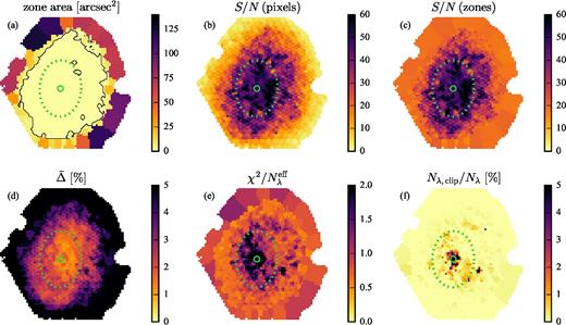
Maps with fit quality indicators of NGC 1667 (CALIFA 0140). A dotted ellipse marks the 1 HLR area, and a small circle marks the galaxy centre. See Table 1 for a brief description of each map.
4.5.1 Data quality maps
Before running the spectra through starlight, some pre-processing is necessary. The most basic is flagging spaxels that we do not want to apply the synthesis to. That includes spaxels with artefacts, foreground objects and very low S/N spaxels (<3). These become masked regions in the maps, where there is no data, appearing white in Figs 2 and 4. The mask is stored in the bad pixel map.
As discussed in Section 3.1, and detailed in section 3.2 of Cid Fernandes et al. (2013), the spaxels with S/N lower than 20 are then binned into Voronoi zones. The zones map assigns a zone number to each pixel, so that if two or more pixels are contained in a given zone, then they share the same number.
Fig. 4(a) shows the area of the Voronoi zones for our example galaxy. As expected, the outer parts of the galaxy have larger zones. The black contour indicates the region where the zones are composed of a single pixel, reaching approximately 2 HLR of the galaxy in this case. This map may be used, for example, to calculate the total mass in each zone. It is also used in the dezonification procedure explained in Section 4.4.2.
Fig. 4(b) shows the pixel-by-pixel S/N ratio in the 5635 ± 45 Å band. The outer parts of the galaxy have S/N well below 10. With the Voronoi binning all the spectra have S/N > 20, as can be seen in Fig. 4(c).
4.5.2 Fit quality maps
Usually, one would resort to χ2 to check the quality of the fit. However, χ2 is closely tied to the uncertainty of the spectra (ελ), which is sometimes difficult to estimate precisely. Due to the clipping algorithm, discussed below, the number of measurements effectively used in the fit (|$N_\lambda ^\mathrm{eff}$|) varies between the spaxels. Therefore, we use |$\chi ^2/N_\lambda ^\mathrm{eff}$| to be able to compare the fit statistic between them. Inspection of Fig. 4(e) may lead to the wrong conclusion that the spectral fits are worse in the nuclear regions than outside, but the larger |$\chi ^2/N_\lambda ^\mathrm{eff}$| values in those regions is because of smaller errors (larger S/N, as seen in panel c), not worse fits. The mean absolute deviation |$\overline{\Delta }$| does not depend explicitly on the uncertainties, so its map in Fig. 4(a) conveys a more appropriate measure of the fit quality.
Another useful quantity to keep track of is the amount of clipping done by starlight during the fit. If some wavelengths have fluxes that are outliers, over ±4 ελ off the model during the fit, they are flagged as clipped, and not used in the fit anymore. This is enforced to keep artefacts and non-masked emission lines from messing up the fit. The fraction of clipped wavelengths, given by Nλ, clip/Nλ, is shown in Fig. 4(f). For CALIFA 0140, the median fraction of clipping is 3.5 per cent, with very few going over 5 per cent. Nevertheless, given that these are usually only a handful among the thousands of pixels, they are usually irrelevant for statistics that take large slices of the maps.
4.5.3 Uncertainties
starlight does not provide error estimates in its output. These uncertainties are usually explored by perturbing the data according to some prescription related to observational and calibration errors, and performing the spectral synthesis several times (e.g. Cid Fernandes et al. 2005).
It is not practical, in our case, to run the synthesis code dozens of times for all spectra from CALIFA. We can, however, use the simulations by Cid Fernandes et al. (2014) to estimate the uncertainties associated with the physical properties obtained by starlight. The simulations were performed using data from a single galaxy, CALIFA 0277. The spectra were perturbed in different ways to estimate the effects of noise, calibration issues and multiplicity of solutions.
Table 3 lists estimated uncertainties associated with the maps in our catalogue. These values are based on the OR1 simulations in Cid Fernandes et al. (2014), in which Gaussian noise with amplitude given by the error in fluxes was injected in the data. The uncertainties are obtained by taking the standard deviation of the difference between the results from perturbed and original spectra. Except for xY, v⋆ and σ⋆, the uncertainties are logarithmic, independent of scale. That means the uncertainties in log Σ⋆ and in |$\log \Sigma ^\prime _\star$| are the same as the uncertainties for log M⋆ given in the table.
Estimated uncertainties of physical quantities, obtained by simulations (Cid Fernandes et al. 2014).
| Uncertainty | ||
|---|---|---|
| Quantity | 20 < S/N < 30 | 40 < S/N < 50 |
| log M⋆ | 0.09 | 0.04 |
| 〈log t〉L | 0.08 | 0.05 |
| 〈log t〉M | 0.15 | 0.07 |
| 〈log Z〉L | 0.08 | 0.05 |
| 〈log Z〉M | 0.12 | 0.07 |
| log SFR | 0.16 | 0.14 |
| xY | 0.03 | 0.01 |
| τV | 0.05 | 0.02 |
| v⋆ [km s−1] | 19 | 9 |
| σ⋆ [km s−1] | 22 | 10 |
Table 3 complements and expands upon a similar table presented in Cid Fernandes et al. (2014). While in that paper the uncertainties were evaluated considering all zones of the galaxy, here we break them into two bins in S/N, one for zones where 20 < S/N < 30, and another one for 40 < S/N < 50, which roughly translates to outer and inner regions of galaxies, respectively (see Fig. 4 c for an example). We find that uncertainties decrease by typically a factor of 2 from the high to the low S/N bin. Uncertainties for individual zones may be obtained by interpolating the values given in Table 3, and using the S/N diagnostic maps. Naturally, these uncertainty estimates must be interpreted as approximate, as they are based on experiments with a single galaxy, and do not take into consideration sources of error other than random noise (like the continuum calibration, also explored by Cid Fernandes et al. 2014).
An independent and more empirical estimate of the uncertainties may be obtained from the catalogue data itself, by comparing regions known to have similar spectra, as those along fixed radial bins in elliptical galaxies, or in the bulges of spirals. This recipe is explored in Section 5.1.1 for CALIFA 0140.
4.6 Integrated spectral analysis
We now turn to the properties derived from the integrated spectra in our catalogue (i.e. simulating a single-beam observation for each galaxy). In the following, we compare physical properties obtained directly from the integrated spectra to the same properties obtained by integrating the spatially resolved results. Since there is only one integrated spectrum per object, we must thus set aside the analysis of one single sample galaxy and consider all galaxies in our main sample.
Fig. 5(a) shows that the total stellar mass M⋆ obtained from the integrated spectra and integrated spatially resolved masses agree remarkably well.
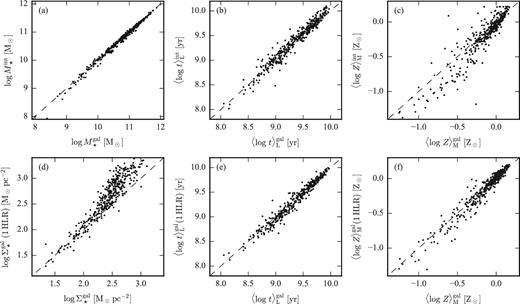
Properties from integrated spectra (superscript ‘int’) versus spatially resolved properties (superscript ‘gal’) for all galaxies in the sample. Panel (a): mass obtained from the integrated spectra against the total mass in the integral of mass surface density map. Panel (b): luminosity-weighted stellar age from the integrated spectra against the mean of stellar ages of all pixels. Panel (c): the same as panel (b), but for mass-weighted stellar metallicity. Panel (d): Mean stellar mass surface density of the whole galaxies against the mean in a ring of 1 HLR around the galaxy nucleus. Panel (e): the same as panel (d), but for luminosity-weighted stellar age. Panel (f): the same as panel (d), but for mass-weighted stellar Metallicity. The dashed lines show the y = x diagonal.
In the lower panels of Fig. 5, we present a comparison between the mean values over the whole galaxy to the mean over a ring at 1 ± 0.1 HLR from the nucleus. The plots show that, for stellar ages and metallicities, the value at 1 HLR is a good proxy for the mean of the whole galaxy. The same is not strictly valid for Σ⋆ (Fig. 5). This happens because the mean stellar mass surface density of a galaxy is not a well-defined value. Given that Σ⋆ decreases with the radius, depending on which radius is chosen as the ‘boundary’ of the galaxy, the surface density can become arbitrarily small. The galaxies of the sample were observed typically up to ∼2.5 HLR. Calculating the average over 2 HLR, for example, moves the points closer to the diagonal. These results confirm what was obtained by González Delgado et al. (2014a), who used the first 107 galaxies observed by CALIFA to perform this same kind of integrated versus resolved analysis.
4.7 Comparison of results with different bases
All examples presented in this paper were obtained with base GMe, described in Section 3.2. As mentioned there, our catalogue also offers results derived with CBe. Previous papers in this series combining CALIFA data with a starlight analysis have compared results obtained with these two bases, drawn from independent sets of evolutionary synthesis models (Cid Fernandes et al. 2014; González Delgado et al. 2015c, 2016). In the interest of completeness, and also to update these previous comparisons to our final sample, Fig. 6 compares properties derived with these two bases, for all 395 galaxies of the main sample. These properties were averaged in radial bins up to 2.5 HLR, in steps of 0.1 HLR. See Section 5.1.1 for more details on radial profiles. The averaging strategy for intensive quantities is the same adopted in the previous section, using equation (10).
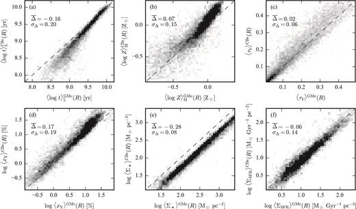
Comparison between the synthesis results using bases GMe and CBe. The panels show 2D histograms of values averaged in radial bins of all 395 maps of the main sample. The horizontal and vertical axes are values obtained using GMe and CBe, respectively. In each panel, we also show the mean and standard deviations of the difference between CBe and GMe. (a) Luminosity-weighted mean stellar age. (b) Mass-weighted mean stellar metallicity. (c) Dust attenuation. (d) Fraction of light in populations younger than 32 Myr. (e) Stellar mass surface density. (f) SFR surface density.
Panels (a)–(d) of Fig. 6 compare the intensive properties 〈log t〉L (panel a), 〈log Z〉M (b), τV (c) and the fraction of light in stellar populations younger than 32 Myr (xY, d) obtained with bases GMe (horizontal axis) and CBe (vertical axis). The other panels compare the results for Σ⋆ (panel e), and ΣSFR (f), both of which are extensive and IMF-sensitive quantities. In all panels, the mean (|$\overline{\Delta }$|) and standard deviation (|$\sigma _\Delta$|) of the Δ ≡ y − x = CBe − GMe difference are indicated.
The results in Fig. 6 agree with our previous comparisons for smaller samples. Mean stellar ages using CBe are 0.16 dex lower, on average. As indicated by the tendency of the offset to increase towards smaller values of 〈log t〉L in panel (a), the difference is mostly due to the fact that young stellar populations come out somewhat stronger with CBe than with GMe, as confirmed in panel (d). Metallicities are somewhat larger when using CBe because its base models reach higher Z than GMe, while the dust attenuation is essentially the same (|$\overline{\Delta }\tau _V = 0.02$|). The stellar mass surface density is lower by a factor of ∼2 when using CBe, reflecting the different IMF used in each base. Differences in ΣSFR values, however, are not as large, with an offset of only 0.06 dex. As seen above in the xY comparison, the fraction of mass in young stellar populations is higher with CBe, which compensates for the lower absolute mass due to differences between the Chabrier and Salpeter IMFs.
Despite the non-negligible differences between bases CBe and GMe, the general results are essentially the same. There are, naturally, systematic offsets in the properties derived with these two sets of models, but these are ultimately not relevant in a comparative analysis, which is essentially what one aims when studying spatial variations of properties such as mean stellar age, metallicity or attenuation caused by dust.
5 USING THE CATALOGUE
The data in our PyCASSO database can be used in a variety of ways to address a wide ranging spectrum of questions. This section gives concrete examples of the kind of work that can be carried out with some simple processing of the maps made publicly available, as described in Section 4.3.
An underlying characteristic of all examples below is that they explore the statistical power of the database, be it using all 316 960 zones in all 395 galaxies from the main sample, in subsamples focusing on certain types of galaxies, or even in single galaxies, which become statistical samples themselves with IFS data. This is not only a sensible approach, but a firmly established working philosophy within the stellar population synthesis community, which, acknowledging the several uncertainties involved in properties retrieved from single spectra, has long vouched for a statistical approach (Panter et al. 2007; Cid Fernandes et al. 2013).
Examples of how to use our database for single galaxies are explored in Section 5.1, while Section 5.2 presents examples of what can be done for samples of galaxies. As anticipated in the introduction (and as already done in Fig. 5), we take the opportunity to update some of the results obtained in our own earlier work.
5.1 Examples of usage for a single galaxy
Maps such as those in Fig. 2 are good for a global appreciation of the results and locating particular spots of the galaxies, like H ii regions or spiral arms, but they are not convenient to visualize trends and gradients. By reducing the dimensionality of the data we may have a better grasp of the behaviour of the physical properties. With radial profiles, we take advantage of both statistics and visualization.
5.1.1 Radial profiles
As an example, Fig. 7 shows radial profiles for some of the physical properties for CALIFA 0140. Each plot shows the values of some property for each zone as grey dots, while the average and ±1σ dispersion in radial bins are shown by the thick and thin solid lines. The radial bins are elliptical annuli with thickness of 0.1 HLR. A vertical dashed line marks the HLR for this galaxy. We warn that this simple statistics may not be the wiser way to treat the physical quantities in this plot, but it suffices for our current illustrative purposes.
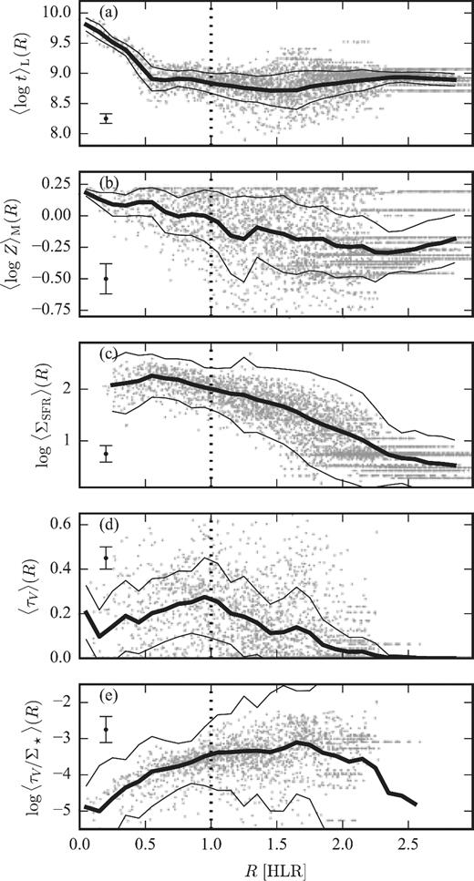
Radial profiles of some physical quantities for CALIFA 0140. The grey dots are the values for individual pixels. The black lines are the mean values in radial bins of width 0.1 HLR, with the 1σ range shown by thin black lines. The vertical dotted line marks 1 HLR. Typical uncertainties associated with these quantities (with the lowest S/N from Table 3) are shown as single error bars at the left side of the plots. See Table 1 for a brief description of these quantities. From top to bottom: luminosity-weighted mean stellar age (a), in (yr); mass-weighted mean stellar metallicity (b), in (Z⊙); SFR surface density (c), in (M⊙ Gyr−1 pc−2); dust attenuation (d), dimensionless; dust-to-stars ratio (e), in arbitrary units.
Panels (a)–(d) show the radial run of 〈log t〉L, 〈log Z〉M, ΣSFR and τV, respectively. The estimated uncertainties, described in Section 4.5.3, are shown as single error bars in each panel. There is substantial scatter in the plots, but the mean radial profiles are well behaved. The mean stellar age (〈log t〉L, Fig. 7(a) shows a clear drop from the centre down to R ∼ 0.7 HLR, where it levels off at a value of about 0.5 Gyr. The mass-weighted mean stellar metallicity 〈log Z〉M decreases more or less steadily by ∼0.4 dex from the nucleus to the outskirts of the galaxy (Fig. 7b). The large scatter is not surprising considering that metallicities are notoriously harder to estimate than ages. The ΣSFR profile (Fig. 7c) peaks at about 0.7 HLR, coinciding with the inflection in the 〈log t〉L profile, decreasing both towards the inner bulge region and the outer disc, as indeed seen (but less clearly so) in the full ΣSFR maps in Fig. 2(g). The dust optical depth9 shows weaker trends, slowly decreasing towards 0 outwards of ∼1 HLR (more or less in tandem with the ΣSFR profile), and slowly decreasing to values around 0.2 in the nucleus.
As anticipated in Section 4.5.3, these profiles may be used to estimate the uncertainties adopted for the properties. For CALIFA 0140, the region inside 0.7 HLR is the bulge of the galaxy. Given that the bulge is fairly symmetrical, the spectra in a radial bin will be roughly equivalent to multiple observations of the same object. This means that the dispersion of the radial profiles serves as an empirical estimate of the uncertainty of these properties. In fact, as the error bars in Fig. 7 illustrate, they are in good agreement with the estimated uncertainties obtained by simulation (Cid Fernandes et al. 2014) presented in Table 3.
The argument of symmetry does not apply to the outer parts of this particular galaxy. The spiral pattern breaks the symmetry, which means the dispersion in the profiles increases outside of 0.7HLR, is caused by the data. Nevertheless, it is still a good estimator of the uncertainty for, e.g. asserting that a gradient in a radial profile is significant.
Further analysis may be done by combining the values present in the catalogue maps. For instance, in Fig. 7(e) we show τV/Σ⋆ to obtain a proxy for the dust-to-stars ratio (itself a proxy for the gas-to-stars ratio given some hypothesis about dust/gas). As shown in González Delgado et al. (2014a), τV profiles generally tend to show negative gradients, which one might read as a tendency for galaxies to be less dusty towards their outer regions. Fig. 7(e) conveys a different impression, however. The rise of τV/Σ⋆ with radius indicates that here are more dust particles per star as one moves away from the nucleus, a trend that may ultimately be reflecting the fact that galaxies are more gas rich towards the outside.
5.1.2 Bulge–disc decomposition in light and mass
Perhaps the most traditional type of surface photometry analysis for spirals is bulge/disc decomposition (Kormendy 1977; Kent 1985). The data distributed in our catalogue allow one to perform this kind of analysis both in light (|$\mathcal {L}_{5635\,{A\!\!\!\!\!^{^\circ}}}$|) and mass (Σ⋆) surface densities.
A morphological analysis of our |$\mathcal {L}_{5635\,{A\!\!\!\!\!^{^\circ}}}$| images (or those produced at any other λ) is not particularly attractive per se, as the image quality of CALIFA is inferior that of publicly available photometry. Indeed, Méndez-Abreu et al. (2017) have recently used SDSS images to perform a morphological analysis of CALIFA galaxies. The mass density maps, however, are clearly of interest, despite the limitations in resolution. Bulge and disc parameters deduced from an analysis of Σ⋆ images are not only more physically meaningful, but also less ambiguous than those derived from the surface brightness, which have the inconvenient property of depending on the wavelength of the image.
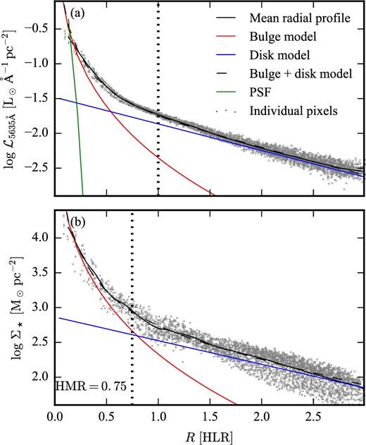
Bulge/disc fit of luminosity (a) and mass (b) surface densities for CALIFA 0127. The morphology models (equations 11 and 12) were fitted to radial profiles of these properties. The central 2.5 arcsec were masked to avoid issues with PSF convolution (the green line shows the PSF profile). The vertical dotted line marks 1 HLR in panel (a) and 1 HMR in panel (b). Blue and red lines in both panels show, respectively, the fitted disc and bulge models, while a dashed black line shows the combined models.
The bulge effective radii obtained from the fits are Re = 0.26 HLR for the |$\mathcal {L}_{5635\,{A\!\!\!\!\!^{^\circ}}}$| profile and 0.24 HLR for Σ⋆ (both of the same order of the PSF width, and so not well resolved), while the disc scales are h = 1.14 HLR for |$\mathcal {L}_{5635\,{A\!\!\!\!\!^{^\circ}}}$| and 1.28 HLR for Σ⋆. It thus seems that the structures have approximately the same sizes whether measured in light or in mass. The relative bulge-to-disc intensity scales, however, change substantially from the |$\mathcal {L}_{5635\,{A\!\!\!\!\!^{^\circ}}}$| to the Σ⋆ fits, as indeed visually evident comparing the vertical scales in Figs 8(a) and (b). The bulge-to-total ratios implied by the fits are B/T = 0.39 in light and 0.55 in mass. In other words, the bulge is more relevant in mass than in light, as expected from its older stellar populations (see Fig. A1) and thus larger mass-to-light ratios.
These differences imply that this galaxy is more compact in mass than in light. A convenient and simple way of quantifying this effect is by comparing the HLRs and half-mass radii (HMRs), respectively. The HMR can be computed using Σ⋆, finding the distance where the cumulative sum of the mass reaches half of its total value. For CALIFA 0127, we obtain HLR = 11.4 arcsec and HMR = 8.5 arcsec, as indicated by the dashed vertical lines in Fig. 8. This galaxy is thus some 25 per cent more compact in mass than in light, as indeed found for most CALIFA galaxies (González Delgado et al. 2015c).
Interestingly, Fig. 8(b) shows that the bulge and disc components have almost exactly the same Σ⋆ at R = 1 HMR. Thus, at least for this galaxy, R = 1 HMR = 0.75 HLR is a good place to divide the galaxy into bulge- and disc-dominated regions. Previous work by our group complies with this recipe, treating regions within 0.5 HLR as bulge-dominated and those at R > 1 HLR as disc-dominated (González Delgado et al. 2014b).
5.2 Examples of usage for many galaxies
While there is much to be learned examining a single galaxy from the sample, the true power of the catalogue becomes evident when we combine large chunks of it. To illustrate this, we begin by investigating half-mass and half-light radii for all galaxies in the sample. Then we move to a little processing, combining radial profiles of all galaxies and deriving a mass–metallicity relation. We finish this section obtaining a Schmidt–Kennicutt (SK)-like relation for a subsample of spiral galaxies.
5.2.1 Half-mass versus half-light radii
As discussed at the end of Section 5.1.2, stellar mass and light are not equally distributed spatially. González Delgado et al. (2015c) have previously compared the HLR and HMR radii of 312 CALIFA galaxies.
Fig. 9 updates that previous result, now for all 395 galaxies in our database, and with the slight changes in the reduction pipeline and starlight analysis described in Section 3. The plot shows HMR and HLR for each galaxy in the sample. For most galaxies, HMR < HLR. A linear fit is drawn as a black line. We find that the galaxies are on average 22 per cent more compact in mass. The difference goes from 18 per cent for elliptical galaxies up to 25 per cent for Sbc galaxies, and decreasing again to 7 per cent for Sd galaxies, in agreement with the results reported by González Delgado et al. (2015c) for a smaller sample.
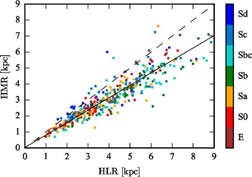
HMR versus HLR for all galaxies in the sample. The y = x line is shown as a black dashed line, while the best linear fit is shown as a continuous black line. The colour of the points denotes the morphological type.
5.2.2 Local relations: stellar mass surface density, age and metallicity
Galaxies come in various shapes and sizes. If we wish to combine and analyse all the galaxies in the sample, we have to somehow homogenize the data. One such way is to take mean radial profiles of the maps, using the HLR as a spatial scale. We use radial bins of 0.1 HLR, from 0 to 2.5 HLR. As seen in Section 5.1.1, we also take the ellipticity and orientation into account.
By using the radial profiles of the maps Σ⋆ and 〈log Z〉M, we can build a mass–metallicity relation (MZR), as seen in Fig. 10(a). The colour of the bins represents the mean value of 〈log t〉L. This plot reproduces one of the results presented by González Delgado et al. (2014b, fig. 2). There we used radial profiles of 300 galaxies. Here, we update that result for 395 galaxies from the main sample.
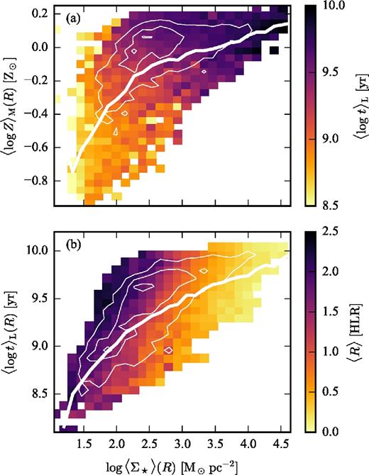
Panel (a): mass–metallicity relation using radial profiles of 〈log Z〉M and Σ⋆, for all galaxies in the sample. The radial bins cover 0 to 2.5 HLR in steps of 0.1 HLR. The background tiles are the mean stellar age in 2D bins. Panel (b): the same as panel (a), but for 〈log t〉L as a function of Σ⋆, with colours representing the mean radial distance. The contours of the density of points are shown in thin white lines, and the mean value of stellar metallicity and age, in bins of mass surface density, is shown as a thick white line, in both panels.
In the bottom panel we show a similar plot, using Σ⋆ and 〈log t〉L, with colours representing the radial distance in HLR units. The white line shows the mean value of stellar metallicity (top) and age (bottom) in bins of mass surface density. The region where the MZR is steeper corresponds to the outer parts of the galaxies, which also tend to be less dense and have younger stellar populations. The MZR becomes flatter in the inner and more dense parts, where the stellar populations are older.
5.2.3 The ΣSFR–τV relation: a proxy for the SK law
One of the most important relations in galaxy studies is the so-called SK law, which relates ΣSFR to surface gas densities (Kennicutt & Evans 2012). Our starlight-based estimates of ΣSFR differ from conventional ones, like those based on the H α luminosity or the far-infrared emission, but at least we have a direct estimate of ΣSFR. The same cannot be said about the gas surface density Σgas, the x-axis in the SK law, which requires measurements of the cold gaseous component in galaxies.
We do, however, have τV at hand. Interpreting it as a proper dust optical depth and making some assumption about grain sizes one may derive dust column densities. Further assuming a constant dust-to-gas ratio one has that τV ∝ Σgas. These are all bold and highly questionable assumptions, of course. Nevertheless they prompt us to investigate the relation between ΣSFR and τV.
In order to do this we first select a subsample of 98 galaxies classified as spiral, non-interacting, with an ellipticity <0.2 – that is, close to being face-on. These galaxies are processed in the same way as the previous section, by calculating radial profiles of ΣSFR and τV. Fig. 11 shows the results, with the colour of the points encoding the radial distance (in HLR units). The black line shows the mean value of mean SFR in bins of τV, with a ±1σ range drawn as thin black lines. If we fit a line to the points, we obtain a slope of ∼1.3. This is amazingly close to the slope of the SK relation (Kennicutt & Evans 2012). A preliminary version of this same relation was presented in Cid Fernandes et al. (2015, fig. 3).
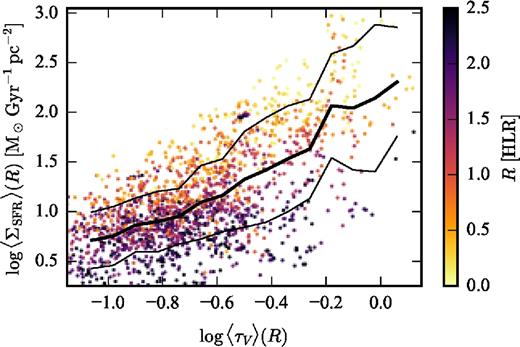
SFR surface density versus the dust extinction (both obtained from our starlight analysis) for 98 face-on spiral galaxies, as derived from images provided in our database. The points are radial means, taken in bins of 0.1 HLR, up to 2.5 HLR. The colour of the points codes for the distance of the bin to the centre of the galaxy, in units of HLR. The mean value of log 〈ΣSFR〉 in bins of log 〈τV〉 is shown as a thick black line, with 1σ range drawn as thin lines. The slope of this line, ∼1.3, is proxy for a SK relation.
6 COMBINING DATA FROM OTHER SOURCES
The combination of our PyCASSO maps with data from other sources should be useful both as an external test on the consistency of the properties offered in our catalogue, and as a way to gain insight into physical processes within galaxies. In this section we explore both approaches. We start by comparing the stellar surface mass densities presented here with those obtained from near-IR imaging (Section 6.1). We then combine our stellar population properties with emission line data to test our SFR estimates and to exemplify how to explore the complementarity of these independent sources of information (Section 6.2). In both cases only publicly available data are used.
6.1 Mass maps from S4G
The Spitzer Survey of Stellar Structure in Galaxies (S4G; Sheth et al. 2010) produced, among other results, maps of the mass in old stars, through imaging in the 3.6 and 4.5 μm bands. We found 35 galaxies present in both PyCASSO and S4G catalogues. In order to compare their Σ⋆ maps to ours, we first downloaded their dust-free surface brightness maps at 3.6 μm (S3.6 μm). As prescribed by Querejeta et al. (2015), a mass-to-light ratio |$M/L_{3.6\, {\mu} \mathrm{m}} = 0.6\,\mathrm{M}_{\odot }\,\mathrm{L}^{-1}_{\odot }$| was used to transform S3.6 μm to stellar surface mass densities. The images were then aligned to ours assuming the centroids in the infrared and optical are at the same position, and radial profiles |$\Sigma _\star ^\mathrm{S^4G} (R)$| were computed exactly as described in Section 5.1.1.
The comparison between the mass surface density from our catalogue and S4G is shown in Fig. 12. Because S4G assumes a Chabrier IMF, we use the CBe base maps. On average these completely independent estimates of Σ⋆ differ by 0.20 dex, with an rms of 0.21 dex, compatible with the expected uncertainties of 0.08 and 0.1 dex from starlight and S4G, respectively.
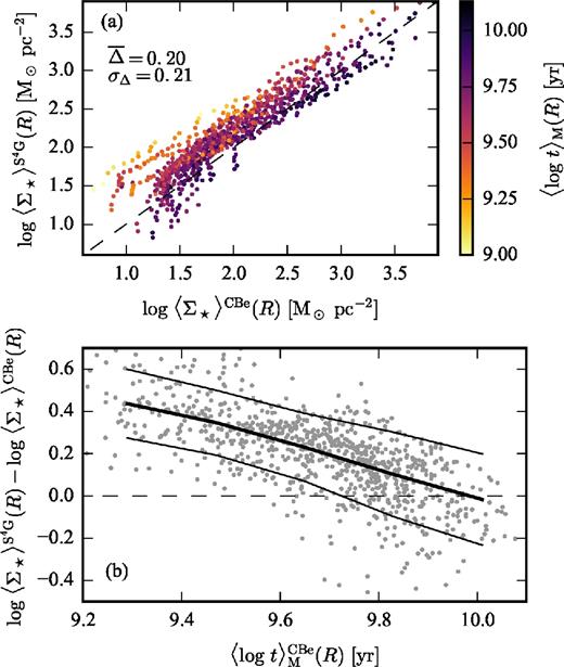
Comparison between stellar mass surface density of 35 galaxies from PyCASSO (using base CBe) and S4G. Each point is the average in an elliptical annulus around the centre of the galaxy. (a) S4G versus PyCASSO. The colour of the points indicates the mass-weighted mean stellar age, 〈log t〉M. (b) Difference between the (logarithmic) masses in both samples, as a function of mass-weighted mean stellar age. The thick black line shows the median in bins of age, and the thin lines indicate the ±1σ dispersion.
There is, however, a clear trend for the difference to increase as Σ⋆ decrease. The mass-weighted mean stellar age (〈log t〉M), coded by the colours in Fig. 12(a), help us understand what is behind this trend. As shown in Fig. 12(b), the S4G and PyCASSO masses are essentially identical as when ∼1010 yr populations dominate the mass in stars. As the contribution of younger populations increases the two estimates start to diverge, reaching a difference of ∼0.4 dex in the extreme cases. The excellent agreement in Σ⋆ for large values of 〈log t〉M is expected, as Querejeta et al. (2015) assumes the light in 3.6 μm comes from old populations, a hypothesis that is encoded in the constant value adopted for M/L3.6 μm. The offset for younger regions is not much larger than the expected uncertainties in the Σ⋆ estimates, and can be improved with a small age-dependent correction to M/L3.6 μm.
6.2 Emission lines from Pipe3D
Pipe3D (Sánchez et al. 2016b) is a pipeline that derives stellar and ionized gas properties from IFS. It uses FIT3D (Sánchez et al. 2016a), a spectral synthesis tool, to model the stellar continuum. The results of Pipe3D applied to 200 galaxies (V500 setup) from CALIFA DR2 (García-Benito et al. 2015) are publicly available at the CALIFA web site.10 We combine the emission line results from Pipe3D to PyCASSO stellar data to explore the gas properties in relation to those of the underlying stellar populations.
When considering a combination of PyCASSO and Pipe3D data, some issues should be noted. The data reduction changed from CALIFA DR2 to DR3. The cubes are not spatially compatible. The techniques used in Pipe3D were implemented independently of this work. Also, Pipe3D used V500 cubes, while we used COMBO cubes. All these characteristics mean that, while using data from the same survey, Pipe3D and PyCASSO are data sets different enough so that a comparison between them is not trivial.
To match the cubes from both sources, we take a 58 × 58 pixels slice around the reference pixel in each fits file, taking advantage of the same pixel scale and orientation in both cases. This allows us to compare results pixel by pixel,11 as well as using radial bins. We exclude galaxies that are morphologically irregular or interacting to avoid problems with the centroid in the reference pixel. The final selection contains 166 galaxies present in both samples.
6.2.1 Star formation rates
As a first application, we may obtain the SFR from the maps of H α emission. This is a measurement of SFR using a region of spectra that is ignored by starlight, being a totally independent measurement. It is therefore instructive to compare these two estimates, following Asari et al. (2007). This is the first time this type of study is done for spatially resolved data.
The SFR is directly converted from H α luminosity using the standard linear relation from Kennicutt (1998), the same used by Sánchez et al. (2016b) to compare their results to other works. The H α fluxes are first corrected for dust attenuation using the Cardelli et al. (1989) law, with RV = 3.1. In this process, we assume an intrinsic ratio H α/H β = 2.86. We mask pixels where S/N < 5 in H α or H β. Pixels where WH α < 14 Å are also masked, to ensure the H α emission is dominated by SF (Lacerda et al., in preparation). The dereddened H α surface brightness translates straightforwardly to ΣSFR, H α, which is then averaged in radial bins of 0.1 HLR, between 0 and 2.5 HLR.
Fig. 13 compares ΣSFR, H α with our starlight-based ΣSFR. The values from both sources agree remarkably well, with virtually no offset. The scatter in this plot, 0.28 dex, is close to the estimated uncertainty of ΣSFR in Table 3. Points in Fig. 13 are colour-coded by |$\tau _V^\mathrm{neb}$|, the optical depth derived from the observed Balmer decrement. We see that |$\tau _V^\mathrm{neb}$| increases with increasing ΣSFR, as expected from the pseudo SK law previously investigated in Fig. 11 in the context of stellar properties alone. This remarkable agreement gives us confidence that the SFR from the PyCASSO database can be used not only for star-forming galaxies, but for other types of galaxies where H α is unrelated to SF.
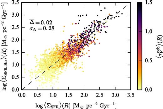
Comparison between the SFR surface density from 166 galaxies in PyCASSO and Pipe3D catalogues. Each point represents an elliptical annulus around the nucleus, going from 0 to 2.5 HLR in steps of 0.1 HLR. The points are coloured according to the mean nebular attenuation.
6.2.2 The WHAN diagram
Still using Pipe3D data, we explore the classification scheme in the WHAN diagram, which plots the equivalent width of H α (WH α) as a function of the ratio between the fluxes in the lines of [N ii]λ6584 and H α. This is a diagnostic diagram proposed by Cid Fernandes et al. (2011) to distinguish among the main ionization sources behind galaxy spectra. SF and AGNs are separated by vertical lines (constant |$[\mathrm{N\, {\small II}}]/\mathrm{H}\,\alpha$|) in this diagram, while sources located below WH α = 3 Å are associated with photoionization by HOLMES.
We extrapolate the original intent of the WHAN diagram by plotting not whole galaxies, but regions of galaxies. In Fig. 14, we have 2D histograms of all pixels of the 166 galaxies matched to Pipe3D. Bin colours in each panel represent the average luminosity-weighted stellar age (〈log t〉L, panel a), specific star formation rate (sSFR, panel b) and distance to the nucleus in units of HLR (panel c); only bins with five points or more are plotted. Contours show the logarithm of the density of points. The WH α = 3 Å line separating HOLMES-ionized gas from SF and AGN regions is indicated. Lines at |$[\mathrm{N\, {\small II}}]/\mathrm{H}\,\alpha = -0.4$| and −0.1 separate SF from AGN regions according to the criteria of Stasińska et al. (2006) and Kewley et al. (2001), respectively, as explained in Cid Fernandes et al. (2010).
![Histogram of equivalent width of H α versus the line ratio $[\mathrm{N\, {\small II}}]/\mathrm{H}\,\alpha$, known as WHAN diagram, using all pixels (no radial binning) from 166 galaxies matched to Pipe3D maps. The colour of the bins represent the mean value of luminosity-weighted mean stellar age (panel a), specific star formation rate (panel b) and radial distance (panel c). Each bin has at least five data points. White contours indicate the logarithm of the density of data points. Blue lines separate the WHAN diagram in the classes SF (star-forming), AGNs and HOLMES. The horizontal continuous line shows the WH α = 3 Å limit for HOLMES. The dashed and dotted vertical lines are equivalent to the Stasińska et al. (2006) and Kewley et al. (2001) SF/AGN dividing lines, respectively.](https://oup.silverchair-cdn.com/oup/backfile/Content_public/Journal/mnras/471/3/10.1093_mnras_stx1805/1/m_stx1805fig14.jpeg?Expires=1716425514&Signature=pGqmnDK2uUOB6pnZAcaWSTtAqs1egYU2asr3TKIuSlfKabxBtDAaR-4jXzOFPjyoXF3SPuJGFWVZZD4kOgGou9hjKoUM1PqnuVWphK4UDS3-HGx9ugQC8RnXNQPc64bTvt0cpO8hnROltlqyW25NJYXQ2Ox2tY1il3kZV5JPFyJ1fJ3HaaVn~o6-Kuc3FYTJL-HjvrsH2B01wqCQAC5S6HmnGtSjeopcPEMQYnI6YTbPwbnNNQ5-mRslaQfEeeVX8XavhLz9eOX8W9PpRA8WS21XVXAYGmOFYjrVej7C3ZWIuNtPkoTULRhxaz4NPCvWzWwKvXTzgh8-Mqzs~HEuyA__&Key-Pair-Id=APKAIE5G5CRDK6RD3PGA)
Histogram of equivalent width of H α versus the line ratio |$[\mathrm{N\, {\small II}}]/\mathrm{H}\,\alpha$|, known as WHAN diagram, using all pixels (no radial binning) from 166 galaxies matched to Pipe3D maps. The colour of the bins represent the mean value of luminosity-weighted mean stellar age (panel a), specific star formation rate (panel b) and radial distance (panel c). Each bin has at least five data points. White contours indicate the logarithm of the density of data points. Blue lines separate the WHAN diagram in the classes SF (star-forming), AGNs and HOLMES. The horizontal continuous line shows the WH α = 3 Å limit for HOLMES. The dashed and dotted vertical lines are equivalent to the Stasińska et al. (2006) and Kewley et al. (2001) SF/AGN dividing lines, respectively.
In Fig. 14(a), we can see that the HOLMES-dominated regions in the WHAN diagram are composed of old stellar populations. Those regions also have the lowest sSFR, as seen in Fig. 14(b). This might not be surprising, since WH α is a proxy for sSFR. This is only true, however, for systems where H α is produced by H ii regions. In contrast, the sSFR measured from the stellar continuum can be used to estimate SFRs in systems where H α is dominated by radiation fields other than young stars, such as AGNs and HOLMES. Fig. 14(c) shows that the region in the WHAN diagram dubbed AGNs is populated not only by the nuclear parts of galaxies, but also by off-nuclear regions. We expect those at low R to be bona fide AGNs, while at higher R the ionization field is most likely a mixture of H ii regions and HOLMES (see Lacerda et al., in preparation).
7 CONCLUSIONS
We have presented a value-added catalogue, publicly available at http://pycasso.ufsc.br/, for CALIFA galaxies analysed with the spectral synthesis code starlight and the pycasso pipeline. The CALIFA IFS sample is representative of galaxies in the local Universe at 0.005 < z < 0.03. Our catalogue is comprised of 445 galaxies from the CALIFA Data Release 3 with COMBO data. From these, 395 are taken from the mother sample, the remaining are from the extended sample.
Our public data contains maps of stellar mass surface densities, mean stellar ages and metallicities, stellar dust attenuation, SFRs, and kinematics. We have provided a road map on how to read and interpret each physical-property image on our catalogue, and given a few examples of how to access the data in the electronic files. Since our analysis is based on spectra that have been binned with Voronoi tessellation to increase the signal-to-noise ratio, we also discuss how one may dezonify (or pixelize) the information on Voronoi zones.
We have also shown how to obtain radial profiles from our maps. Radial profiles are useful representations of 2D maps, and we showcase their usefulness by separating a galaxy’s bulge and disc both in its light and stellar mass profiles. This case study agrees with our previous results (González Delgado et al. 2015c) that galaxies are more compact in mass than in light.
We have used our catalogue to update and revisit a few of our former results, like the relation between HMRs and HLRs, and local relations between stellar mass surface density, age and metallicity. A few previously unexplored results were also presented, like a pseudo SK relation between the SFR surface density and the dust optical depth obtained using only stellar continuum information.
Finally, in order to illustrate the potential of the catalogue when used in conjunction with complementary information from other databases, we have combined it with publicly available data from the S4G and Pipe3D databases. Using emission line measurements for 166 galaxies from Pipe3D, we compare the sSFR from the stellar continuum to that obtained from H α, finding that the two agree with a factor of 2. We also investigate how galaxy pixels populate the WHAN diagram, which can distinguish the ionization by SF, AGNs or HOLMES in full galaxies. We show that the HOLMES/SF scenario is compatible with the stellar population ages and sSFR in the PyCASSO database. These example applications demonstrate the catalogue should be a useful tool to gain insight into galaxy physics.
Acknowledgements
ALdA, NVA, RCF and EADL acknowledge the support from the Coordenação de Aperfeiçoamento de Pessoal de Nivel Superior (CAPES) Ciência sem Fronteiras - Pesquisador Visitante Especial (CsF-PVE) project 88881.068116/2014-01.
CALIFA is the first legacy survey carried out at Calar Alto. The CALIFA collaboration would like to thank the Instituto de Astrofísica de Andalucía - Centro Superior de Investigaciones Científicas (IAA-CSIC) and Max Planck Institut für Astronomie - Max Planck Gesellschaft (MPIA-MPG) as major partners of the observatory, and CAHA itself, for the unique access to telescope time and support in manpower and infrastructures. We also thank the CAHA staff for the dedication to this project.
We thank the support from the Spanish Ministerio de Economía y Competitividad, through projects AYA2016-77846-P, AYA2014-57490-P, AYA2010-15081 and Junta de Andalucía FQ1580. We also thank the Viabilidad, Diseño, Acceso y Mejora funding program, ICTS-2009-10, for funding the data acquisition of this project. ALdA, EADL and RCF thanks the hospitality of the IAA and the support of Conselho Nacional de Pesquisa (CNPq). RGD acknowledges the support of CNPq.
We thank the referee for comments that substantially improved this manuscript.
This research used astropy, a community-developed core python package for Astronomy (Astropy Collaboration 2013).
Assuming a Salpeter IMF.
Morphological classification performed by the collaboration is available as ancillary data tables, at the CALIFA DR3 website (http://www.caha.es/CALIFA/public_html/?q=content/dr3-tables).
The Charlot & Bruzual (2007) models are available at http://www.bruzual.org/∼gbruzual/cb07.
The bad pixels values are set to zero, which may be a valid value depending on the map. A map indicating which pixels are bad is also provided, to help in those cases.
SDSS DR13 image obtained from SkyServer.
The HLR is straightforwardly computed by finding the distance where the cumulative sum of the luminosity reaches half of its total value. This is done along the major axis of ellipses with ellipticity and position angle defined by the moments of the image (Stoughton et al. 2002). Note that in this work we calculate HLR using the |$\mathcal {L}_{5635\,{A\!\!\!\!\!^{^\circ}}}$| map, which may or may not have masked regions. Also, in some cases the FoV does not cover the whole galaxy. The HLR is a convenient spatial metric, particularly useful when comparing results obtained for different galaxies.
Also known as SFR intensity in some works.
Stellar kinematics maps from Falcón-Barroso et al. (2017) are available at http://www.caha.es/CALIFA/public_html/?q=content/science-dataproducts.
Note that starlight assumes a dust screen and finds the effective attenuation at each zone of a CALIFA galaxy. Thus, one should be careful when interpreting τV as the dust optical depth. In addition, the arithmetic averaging of τV may be misleading: the radial profiles show the typical value of τV at a given radius, but not the effective attenuation one would obtain if analysing the co-added spectra in a ring.
CALIFA science dataproducts available at http://www.caha.es/CALIFA/public_html/?q=content/science-dataproducts.
Pipe3D used a different segmentation scheme, named CS-method. The maps are reconstructed using a form of dezonification similar to ours.
REFERENCES
APPENDIX A: OTHER GALAXIES
This appendix shows a few more examples of maps available in the PyCASSO database (http://pycasso.ufsc.br/) presented in this paper. Figs A1 to A8 are sorted according to morphological type, from an elliptical galaxy to a merger.
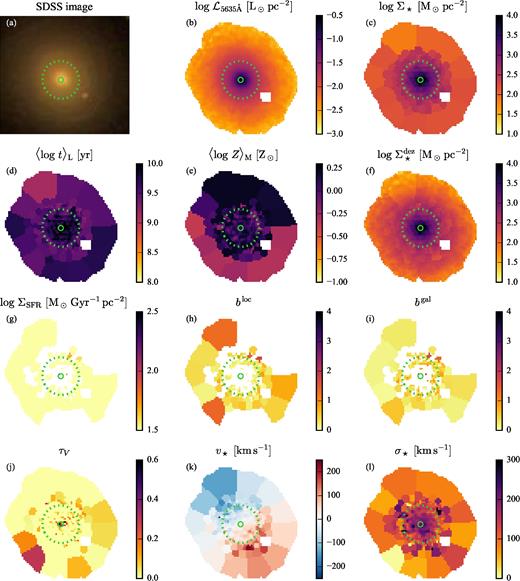
Maps of selected physical properties for the elliptical galaxy NGC 1349 (CALIFA 0127). A dotted ellipse marks the 1 HLR area.
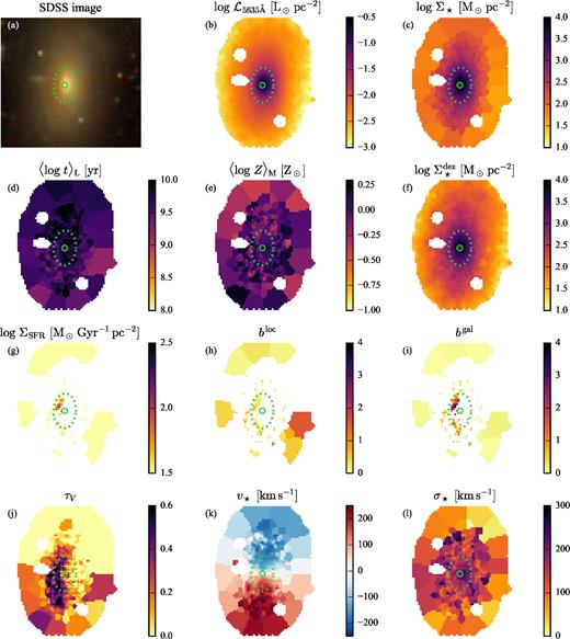
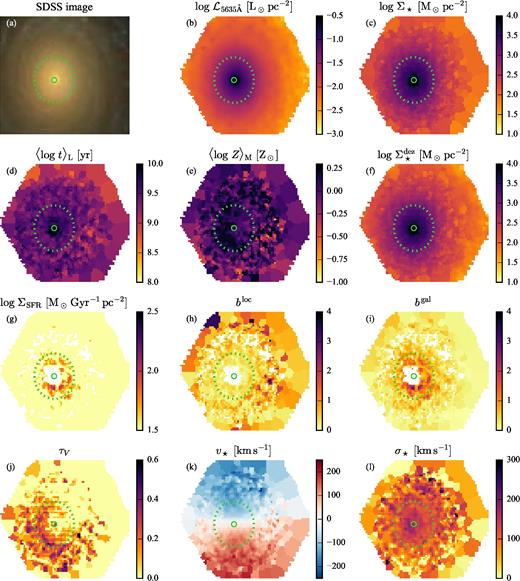
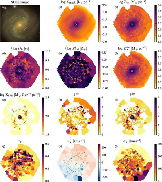
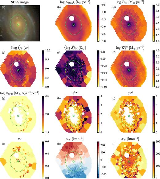
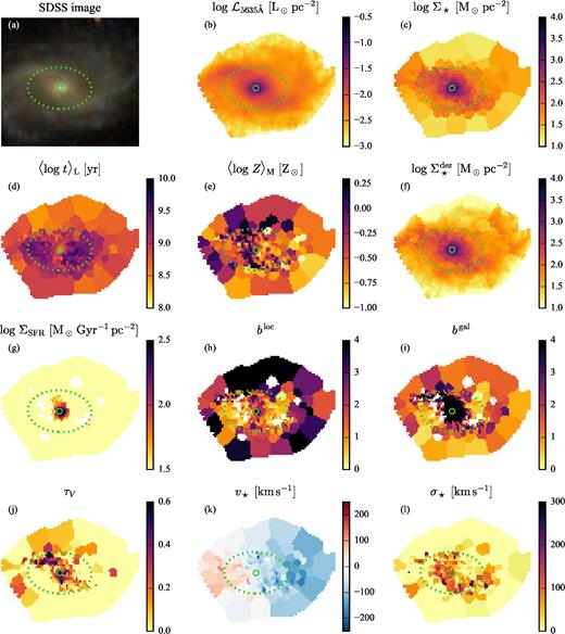
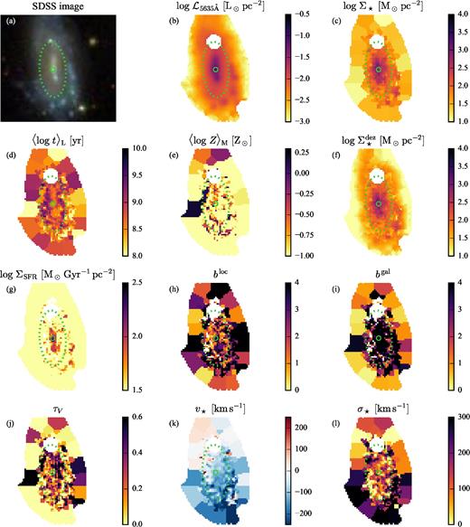
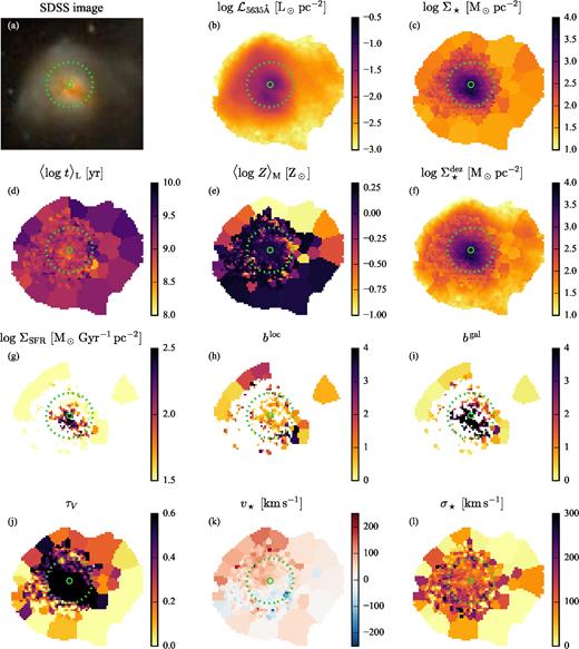
