


Abstract
Binary black holes (BBHs) may form both through isolated binary evolution and through dynamical interactions in dense stellar environments. The formation channel leaves an imprint on the alignment between the BH spins and the orbital angular momentum. Gravitational waves (GW) from these systems directly encode information about the spin–orbit misalignment angles, allowing them to be (weakly) constrained. Identifying subpopulations of spinning BBHs will inform us about compact binary formation and evolution. We simulate a mixed population of BBHs with spin–orbit misalignments modelled under a range of assumptions. We then develop a hierarchical analysis and apply it to mock GW observations of these populations. Assuming a population with dimensionless spin magnitudes of χ = 0.7, we show that tens of observations will make it possible to distinguish the presence of subpopulations of coalescing binary black holes based on their spin orientations. With 100 observations, it will be possible to infer the relative fraction of coalescing BBHs with isotropic spin directions (corresponding to dynamical formation in our models) with a fractional uncertainty of ∼40 per cent. Meanwhile, only ∼5 observations are sufficient to distinguish between extreme models – all BBHs either having exactly aligned spins or isotropic spin directions.
1 INTRODUCTION
Compact binaries containing two stellar-mass black holes (BHs) can form as the end point of isolated binary evolution, or via dynamical interactions in dense stellar environments (see e.g. Mandel & O'Shaughnessy 2010; Abbott et al. 2016h, for a review). These binary black holes (BBHs) are a promising source of gravitational waves (GWs) for ground-based detectors such as Advanced LIGO (aLIGO; Aasi et al. 2015), Advanced Virgo (AdV; Acernese et al. 2015) and KAGRA (Aso et al. 2013). Searches of data from the first observing run (Abbott et al. 2016a) of Advanced LIGO (aLIGO) yielded three likely BBH coalescences: GW150914 (Abbott et al. 2016e), GW151226 (Abbott et al. 2016g) and LVT151012 (Abbott et al. 2016c,d). A further BBH coalescence, GW170104, has been reported from the on-going second observing run (Abbott et al. 2017). GW observations give a unique insight into the properties of BBHs. We will examine one of the ways in which BH spin measurements can be used to constrain formation mechanisms.
GW observations inform our understanding of BBH evolution in two ways: from the merger rate and from the properties of the individual systems. The merger rate of BBHs is inferred from the number of detections; it is uncertain as a consequence of the small number of BBH observations so far. Currently, merger rates are estimated to be 12–213 Gpc−3 yr−1 (Abbott et al. 2016i; Abbott et al. 2017). These rates are broadly consistent with predictions from both population synthesis models of isolated binary evolution (e.g. Voss & Tauris 2003; Lipunov et al. 2009; Dominik et al. 2012; Postnov & Yungelson 2014) and dynamical formation models (e.g. Sigurdsson & Hernquist 1993; Sadowski et al. 2008; Rodriguez et al. 2015). Possible progenitors systems of BBHs, including Cyg X-3 (Belczynski et al. 2013), IC 10 X-1 (Bulik, Belczynski & Prestwich 2011) and NGC 300 X-1 (Crowther et al. 2010), provide some additional limits on BBH merger rates, but extrapolation is hindered by current observational uncertainties.
The parameters of individual systems can be estimated by comparing the measured GW signal with template waveforms (Abbott et al. 2016f). The masses and spins of the BHs can be measured through their influence on the inspiral, merger and ringdown of the system (Finn & Chernoff 1993; Cutler & Flanagan 1994; Poisson & Will 1995). The distribution of parameters observed by aLIGO will encode information about the population of BBHs, and may also help to shed light on their formation channels (O'Shaughnessy et al. 2008; Kelley et al. 2010; Gerosa et al. 2013, 2014; Mandel et al. 2015; Stevenson et al. 2015; Mandel et al. 2017; Vitale et al. 2017).
Stellar-mass BHs are expected to be born spinning, with observations suggesting their dimensionless spin parameters χ take the full range of allowed values between 0 and 1 (McClintock et al. 2011; Fragos & McClintock 2015; Miller & Miller 2015). Stars formed in binaries are expected to have their rotational axis aligned with the orbital angular momentum (e.g. Boss 1988; Albrecht et al. 2007), although there is observational evidence that this is not always the case (e.g. Albrecht et al. 2009, 2014). Even if binaries are born with misaligned spins, there are many processes in binary evolution that can act to align the spin of stars, such as realignment during a stable mass accretion phase (Bardeen & Petterson 1975; Kalogera 2000; King et al. 2005), accretion on to a BH passing through a common-envelope (CE) event (Ivanova et al. 2013) and realignment through tidal interactions in close binaries (e.g. Zahn 1977; Hut 1981).
On the other hand, asymmetric mass loss during supernova explosions can tilt the orbital plane in binaries (Brandt & Podsiadlowski 1995; Kalogera 2000), leading to BH spins being misaligned with respect to the orbital angular momentum vector. Population synthesis studies of BH X-ray binaries predict that these misalignments are generally small (Kalogera 2000), with Fragos et al. (2010) finding that the primary BH is typically misaligned by ≲10°. However, electromagnetic observations of high-mass X-ray binaries containing BHs have hinted that the BHs may be more significantly misaligned (Miller & Miller 2015). One such system is the microquasar V4641 Sgr (Orosz et al. 2001; Martin, Reis & Pringle 2008), where the primary BH has been interpreted to be misaligned by >55°.
Alternatively, BBHs can form dynamically in dense stellar environments such as globular clusters. In these environments, it is expected that the distribution of BBH spin–orbit misalignment angles is isotropic (e.g. Rodriguez et al. 2016). The distribution of BBH spin–orbit misalignments therefore contains information about their formation mechanisms.
Constraints on spin alignment from GW observations so far are weak (Abbott et al. 2016f; Abbott et al. 2016b; Abbott et al. 2016c, 2017). Some configurations, such as anti-aligned spins for GW151226 (Abbott et al. 2016g), are disfavoured; however, there is considerable uncertainty in the spin magnitude and orientation. Determining the spins precisely is difficult because their effects on the waveform can be intrinsically small (especially if the source is viewed face on), and because of degeneracies between the spin and mass parameters (Poisson & Will 1995; Baird et al. 2013; Farr et al. 2016). Although the spins of individual systems are difficult to measure, here we show it is possible to use inferences from multiple systems to build a statistical model for the population (cf. Vitale et al. 2017).
This paper describes how to combine posterior probability density functions on spin–orbit misalignment angles from multiple GW events to explore the underlying population.
We develop a hierarchical analysis in order to combine multiple GW observations of BBH spin–orbit misalignments to give constraints on the fractions of BBHs forming through different channels. We consider different populations of potential spin–orbit misalignments, each representing different assumptions about binary formation, and use the GW observations to infer the fraction of binaries from each population. In the field of exoplanets, similar hierarchical analyses have been used to make inference on the frequency of Earth-like exoplanets from measurements of the period and radius of individual exoplanet candidates (e.g. Foreman-Mackey, Hogg & Morton 2014; Farr et al. 2014a). Other examples of the use of hierarchical analyses in astrophysics include modelling a population of trans-Neptunian objects (Loredo 2004), measurements of spin–orbit misalignments in exoplanets (Naoz, Farr & Rasio 2012), measurements of the eccentricity distribution of exoplanets (Hogg, Myers & Bovy 2010) and the measurement of the mass distribution of galaxy clusters (Lieu et al. 2017).
In Section 2, we introduce our simplified population synthesis models for BBHs, paying special attention to the BH spins. We briefly describe in Section 3 the parameter estimation (PE) pipeline that will be employed to infer the properties (such as misalignment angles) of real GW events, and discuss previous spin-misalignment studies in the literature. We introduce a framework for combining posterior probability density functions on spin–orbit misalignment angles from multiple GW events to explore the underlying population in Section 4. We demonstrate the method using a set of mock GW events in Section 5, and show that tens of observations will be sufficient to distinguish subpopulations of coalescing BBHs, assuming spin magnitudes of ∼0.7. Lower typical BH spin magnitudes would reduce the accuracy with which the spin–orbit misalignment angle can be measured, therefore requiring more observations to extract information about subpopulations. We also show that more extreme models, such as the hypothesis that all BBHs have their spins exactly aligned with the orbital angular momentum, can be ruled out at a 5σ confidence level with only |$\mathcal {O}(5)$| observations of rapidly spinning BBHs. Finally, we conclude and suggest areas that require further study in Section 6.
2 BH SPIN MISALIGNMENT MODELS
Owing to the many uncertainties pertaining to stellar spins and their evolution in a binary, and the fact that keeping track of stellar spin vectors can be computationally intensive, many population synthesis models choose not to include spin evolution. However, the distribution of spins of the final merging BHs is one of the observables that can be measured with the advanced GW detectors. In this section, we therefore implement a simplified population synthesis model to evolve an ensemble of binaries that will be detectable with aLIGO and Advanced Virgo (AdV) and predict their distributions of spin–orbit misalignments. We describe the assumed mass distribution, spin distribution and spin evolution below.
2.1 Mass and spin magnitude distribution
We assume the same simplified mass distribution for all of our models, so that any differences in the final spin distributions are purely due to our assumptions about the spin–orbit misalignments described in the next section. There are many uncertainties in the evolution of isolated massive binaries, including (but not limited to) uncertainties in the initial distributions of the orbital elements (de Mink & Belczynski 2015), the strength of stellar winds in massive stars (Belczynski et al. 2010), the effect of rotation of massive stars on stellar evolution (de Mink et al. 2013; Ramírez-Agudelo et al. 2015), the natal kicks (if any) given to BHs (Repetto, Davies & Sigurdsson 2012; Mandel 2016; Mirabel 2017; Repetto, Igoshev & Nelemans 2017) and the efficiency of the CE (Ivanova et al. 2013; Kruckow et al. 2016). Population synthesis methods are large Monte Carlo simulations using semi-analytic prescriptions in order to explore the effect these uncertainties have on the predicted distributions of compact binaries. Instead, we adopt a number of simplifications that allow us to produce an astrophysically plausible distribution that should not, however, be considered representative of the actual mass distribution of BBHs.
We simulate massive binaries with semi-major axis a drawn from a distribution uniform in ln a (Abt 1983). The components of the binary are a massive primary BH with mass m1 and a secondary star at the end of its main sequence lifetime.
The primary BH was formed from a massive star with zero-age main sequence (ZAMS) mass |$m_1^\mathrm{ZAMS}$| drawn from the initial-mass function (IMF) with a power-law index of −2.35 (Salpeter 1955; Kroupa 2001). The mass ratio of the binary at ZAMS qZAMS is drawn from a flat distribution [0, 1]. The mass of the secondary star is given by |$m_{2}^\mathrm{ZAMS} = q^\mathrm{ZAMS} m_{1}^\mathrm{ZAMS}$|.
We assume that the binary has negligible eccentricity e = 0, appropriate for post-CE systems. In all models, we have assumed that both main-sequence stars in the binary are born with their rotation axis aligned with the orbital angular momentum axis. In general, the first supernova will misalign the spins due to any natal kick imparted on the remnant. There are expected to be mass-transfer phases between the first and second supernovae, which may realign the spins of both the primary BH and the secondary BH progenitors; we vary the assumed degree of realignment in our models.
We assume that BHs receive natal kicks comparable to those received by neutron stars (Hobbs et al. 2005), namely drawn from a Maxwellian with a root-mean-square velocity of ∼250 km s−1. This assumption will lead to the maximum amount of spin misalignment, and may be consistent with neutrino-driven kicks; if the natal kicks are due to asymmetric ejection of baryonic matter, then any fall-back (Fryer et al. 2012) on to BHs during formation will reduce the kick magnitude and thus the spin misalignment.
BH spin magnitudes can take any value 0 ≤ χi < 1, but we set χi = 0.7 for all our BHs. High spin magnitudes are consistent with measurements from X-ray observations (cf. Miller & Miller 2015), and lie towards the upper end of the range allowed by current GW observations (Abbott et al. 2016c, 2017). Such spins are large enough to ensure spin effects on the gravitational waveform are significant, providing an opportunity for us to demonstrate our hierarchical approach, but small enough that we do not have to worry about the validity of the model gravitational waveform. Uncertainties in the relationship between pre-supernova stellar spins and BH spins mean it is not currently possible to produce a realistic distribution of spins from first principles, although a direct translation is often assumed, e.g. by Kushnir et al. (2016). If the distribution of BH spin magnitudes in nature favours smaller values, then more observations will be required to draw the conclusions we find here. The methodology we use here can be extended to models including BH spin magnitudes, which could potentially give us further information regarding formation mechanisms.
After a supernova, we establish whether the binary remains bound, and for those that do, we find the new orbital elements (Blaauw 1961; Brandt & Podsiadlowski 1995; Kalogera 1996). Of the remaining bound systems, we are only interested in those binaries that merge due to the emission of gravitational radiation within a Hubble time, as these are the binaries that are potentially observable with GW detectors.
2.2 Models for spin–orbit misalignment distributions
We model the overall population of BBHs as a mixture of four subpopulations, each of which makes differing assumptions leading to distinct spin–orbit misalignment distributions.
Subpopulation 1: Exactly aligned. We assume that irrespective of all prior processes, both BHs have their spins aligned with the orbital angular momentum vector after the second supernova, such that cos θ1 = cos θ2 = 1. This may be the case if BHs receive no kicks. GW searches often assume BBHs have aligned spins as this simplification makes the search less computationally demanding (Abbott et al. 2016d).
Subpopulation 2: Isotropic/dynamical formation. We assume that BBHs are formed dynamically, such that the distribution of spin angles is isotropic. Initially, isotropic distributions of spins remain isotropic (Schnittman 2004). We still generate the binary mass distribution with our standard approach, so that the only difference in BBHs between this model and the others is the spin distribution.
Subpopulation 3: Alignment before second SN. Motivated by Kalogera (2000), we assume that the spins of both components are aligned with the orbital angular momentum after a CE event and prior to the second supernova. The tilt of the orbital plane caused by the second supernova is then taken to be the spin misalignment angle of both components, i.e. cos θ1 = cos θ2. As we discuss in Section 2.3, these spins freely precess from the time of the second supernova up until merger. This precession somewhat scatters these angles, but leaves them with generally similar values, as seen in Fig. 1.
Subpopulation 4: Alignment of secondary. We follow the standard mass-ratio model with effective tides presented in Gerosa et al. (2013), which assumes that after the first supernova, the secondary is realigned via tides or the CE prior to the second supernova. However, the primary BH is not realigned. Because the binary's orbit shrinks during CE ejection, the kick velocity of the secondary is small relative to its pre-supernova velocity, causing the secondary to be only mildly misaligned (in general θ1 > θ2).
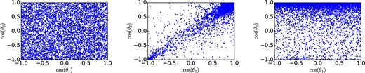
Three of the four astrophysically motivated subpopulations making up our mixture model for BBH spin misalignment angles θ1 and θ2 described in Section 2. Subpopulation 1 (not shown) has both spins perfectly aligned (cos θ1 = cos θ2 = 1), so all points would lie in the top right-hand corner. In subpopulation 2 (left-hand panel), both spins are drawn from an isotropic distribution, and so the samples are distributed uniformly in the plane. In subpopulation 3, BH spins are aligned with the orbital angular momentum just prior to the second supernova. In subpopulation 4, the secondary BH has its spin aligned with the orbital angular momentum prior to the second supernova, whilst the primary is misaligned. See Section 2 for more details. Spins are quoted at a GW frequency of fref = 10 Hz.
We generate several thousand samples from each of these models. We plot samples from the four subpopulations in the {cos θ1, cos θ2} plane of the misalignment angles in Fig. 1. From each of these models, we randomly select 20 mock detected systems (for a total of N = 80) with component masses between 10 and 40 M⊙ (cf. Abbott et al. 2016c); we describe the analysis of these mock GW signals in Section 3. We show the true values of the spin misalignment angles for the mock detected systems in Fig. 2.
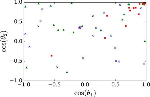
True values of BH spin–orbit misalignment angles cos θ1 and cos θ2 for a mixture of 20 draws from each of our four subpopulations. Exactly aligned systems from subpopulation 1 sit in the upper right-hand corner of this diagram and thus are not shown. Systems drawn from subpopulation 2 are shown as blue crosses, those from subpopulation 3 as red squares and those from subpopulation 4 as green triangles. The injection plotted in Figs 3 and 7 is circled in magenta.
We use a roughly astrophysical distribution of systems with sky positions and inclinations randomly chosen, and distances DL distributed uniformly in volume, |$p(D_\mathrm{L}) \propto D_\mathrm{L}^{2}$|, such that the distribution of signal-to-noise ratio (SNR) ρ is p(ρ) ∝ ρ−4 (Schutz 2011). This approximates the Universe as being static, with constant merger rates per unit time, at the distance scales probed by current detectors. We use a detection threshold (minimum network SNR) of ρmin = 12 (Berry et al. 2015; Abbott et al. 2016a).
2.3 Precession and spin–orbit resonances
After the second supernova, the evolution of the BBH is purely driven by relativistic effects and the orbit decays due to the emission of gravitational radiation (Peters & Mathews 1963; Peters 1964). As the BHs orbit, their spins precess around the total angular momentum (Apostolatos et al. 1994; Blanchet 2014). In order to predict the spin misalignment angles when the frequency of GWs emitted by the binary are high enough (or equivalently when the orbital separation of the binary is sufficiently small) to be in the aLIGO band (fGW > 10 Hz), we take into account the post-Newtonian (PN) evolution of the spins by evolving the ten coupled differential equations given by equations (14)–(17) in Gerosa et al. (2013). We begin our integrations at an orbital separation a = 1000M, and integrate up until fGW = 10 Hz.2
Some of these binaries are attracted to spin–orbit resonances (Schnittman 2004). In particular, the binaries from subpopulation 4 are attracted to the ΔΦ = ±180° resonance, where ΔΦ is the angle between the projection of the two spins on the orbital plane. The current generation of ground-based GW observations are generally insensitive to this angle for BBHs (Schmidt, Ohme & Hannam 2015; Abbott et al. 2016b), and the waveform model we use does not include it, so we focus on distinguishing subpopulations through the better-measured θ1 and θ2 angles.
3 GW PARAMETER ESTIMATION
3.1 Signal analysis and inference
We sample the posterior distribution using the publicly available, Bayesian PE code LALInference (Veitch et al. 2015a).4 For each event we obtain ν ∼ 5000 independent posterior samples. We show an example of the marginalized posterior distribution in {cos θ1, cos θ2} space for one of our 80 events in Fig. 3. Unless otherwise stated, we quote all parameters at a reference frequency fref = 10 Hz.
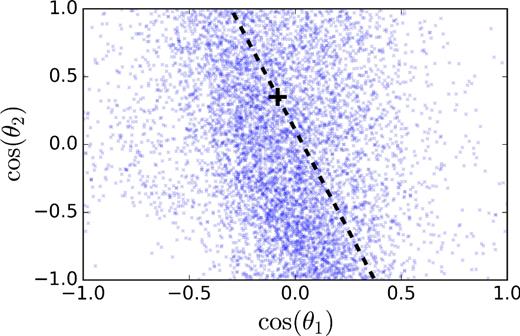
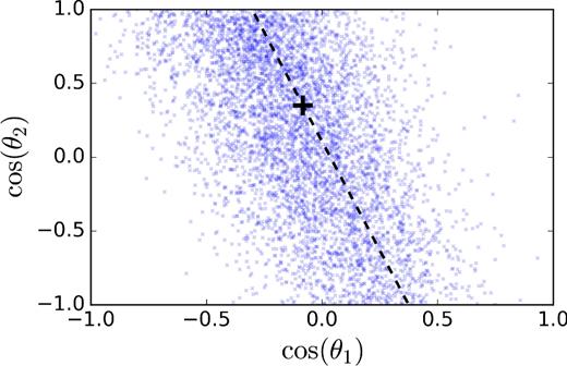
Marginalized posterior samples for one of the 80 events shown in Fig. 2, generated by analysing mock GW data using LALInference. The true spin–orbit misalignments (thick black plus) for this event were cos θ1 = −0.08 and cos θ2 = 0.35, with a network SNR of 15.35. The dashed black diagonal line shows the line of constant χeff.
We sample in the system frame (Farr et al. 2014b), where the binary is parametrized by the masses and spin magnitudes of the two component BHs {mi} and {χi}, the spin misalignment angles {θi}, the angle ΔΦ between the projections of the two spins on the orbital plane, and the angle β between the total and orbital angular momentum vectors. We find, in agreement with similar studies such as Littenberg et al. (2015) and Miller et al. (2015), that there is a strong preference for detecting GWs from nearly face-on binaries, since GW emission is strongest perpendicular to the orbital plane.
Following common practice in PE studies, we use a special realization of Gaussian noise, which is exactly zero in each frequency bin (Veitch, Pürrer & Mandel 2015b; Trifirò et al. 2016). Real GW detector noise will be non-Gaussian and non-stationary, and events will be recovered with non-zero noise.5 Non-zero noise-realizations will mean that in general the maximum likelihood parameters do not match the injection parameters; in the Gaussian limit, however, using a zero noise realization is equivalent to averaging over a large number of random noise realizations, such that these offsets approximately cancel out (cf. Vallisneri 2011). This assumption makes it straightforward to compare the posterior distributions, as differences only arise from the input parameters and not any of the specific noise realization.
3.2 Previous studies
Vitale et al. (2017) study GW measurements of BH spin misalignments in compact binaries containing at least one BH. They consider both BBHs (using IMRPhenomPv2 waveforms as we do here) and neutron star–black hole (NSBH) binaries (using inspiral-only SpinTaylorT4 waveforms). They fit a mixture model allowing for both a preferentially aligned/anti-aligned component and an isotropically misaligned component, excluding aligned/anti-aligned systems. They find that ∼100 detections yield a ∼10 per cent precision for the measured aligned fraction. One of the main limitations of the analysis performed by Vitale et al. (2017) is that they only consider models that are mutually exclusive, although this should not affect their results since the excluded region for their non-aligned model is negligible. Here, all of our formation models overlap in the parameter space of spin–orbit misalignment angles. Therefore, we cannot directly apply the formalism of Vitale et al. (2017). The framework we develop here is able to correctly determine the relative contributions of multiple models, even when those models overlap in parameter space significantly, as expected in practice.
There have also been significant advances in the past few years in the understanding of PN spin–orbit resonances. These resonances occur when BH spins become aligned or anti-aligned with one another and precess in a common plane around the total angular momentum (Schnittman 2004). This causes binaries to be attracted to different points in parameter space identified by ΔΦ, the angle between the projections of the two BH spins on to the orbital plane. Kesden, Sperhake & Berti (2010) have shown that these resonances are effective at capturing binaries with mass ratios 0.4 < q < 1 and spins χi > 0.5. For equal-mass binaries, spin morphologies remain locked with binaries trapped in or out of resonance (Gerosa, Sperhake & Vošmera 2017); however, it is unlikely for astrophysical formation scenarios to produce exactly equal mass binaries, although Marchant et al. (2016) predict nearly equal masses for the chemically homogeneous evolution channel.
Gerosa et al. (2013) show how the family of resonances that BBHs are attracted to can act as a diagnostic of the formation scenario for those binaries. Trifirò et al. (2016) demonstrate that GW measurements of spin misalignments can be used to distinguish between the two resonant families of ΔΦ = 0° and ΔΦ = ±180°. They use a full PE study to show that they can distinguish two families of PN resonances. However, they consider only a small corner of parameter space that contains binaries that will become locked in these PN resonances.
Our study extends on those discussed in several ways:
Rather than focusing on specific systems preferred in previous studies, we use injections from an astrophysically motivated population. Our injections have total masses M = m1 + m2 in the range 10–40 M⊙ and an astrophysical distribution of SNRs.
The misalignment angles of our BHs are given by simple but astrophysically motivated models introduced in Section 2.
For performing PE on individual GW events, we use the inspiral-merger-ringdown gravitational waveform IMRPhenomPv2 model, rather than the inspiral-only waveforms used in some of the earlier studies.
Most importantly, we perform a hierarchical Bayesian analysis on the posterior probability density functions of a mock catalogue of detected events in order to make inferences about the underlying population.
4 HIERARCHICAL ANALYSIS FOR POPULATION INFERENCE
PE on individual GW events yields samples from the posterior distributions for parameters under astrophysical prior constraints. We now wish to combine these individual measurements of BH spin misalignment angles in order to learn about the underlying population, which may act as a diagnostic for binary formation channels and binary evolution scenarios. Importantly, we are able to do this without reanalysing the data for the individual events.
Given a set of reasonable population synthesis model predictions for BBH spin misalignment angles, we would like to learn what mixture of those subpopulations best explains the observed data. Here, we assume that the subpopulation distributions representing different formation channels are known perfectly, and use the same subpopulations that we drew our injections from to set these distributions. Thus, each subpopulation model Λℓ (ℓ ∈ 1…4) corresponds to a known distribution of source parameters |$p(\boldsymbol {\Theta } | \Lambda _\ell )$|. In practice, the uncertainty in the subpopulation models will be one of the challenges in carrying out accurate hierarchical inference.6
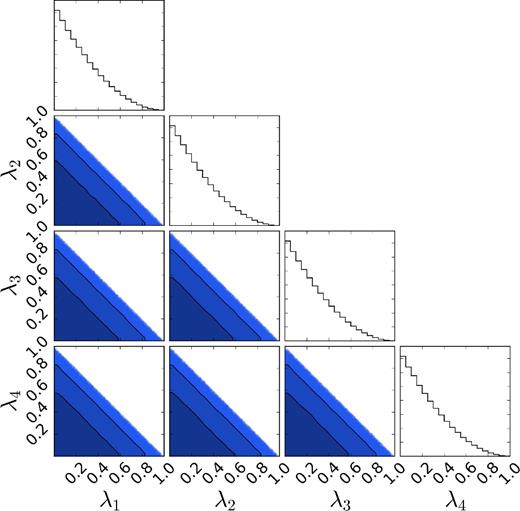
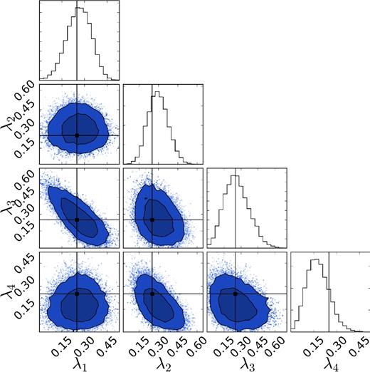
Marginalized 1D and 2D probability density functions for the Dirichlet prior used for the analysis of the λ parameters, which describe the fractional contribution of each of the four subpopulations introduced in Section 2. The constraint λ1 + λ2 + λ3 + λ4 ≡ 1 introduces correlations between parameters. The shaded regions show the 68 per cent (darkest blue) and 95 per cent (middle blue) confidence regions, with the individual posterior samples outside these regions plotted as scatter points (lightest blue).
5 RESULTS
To gain a qualitative understanding of hierarchical modelling on the spin–orbit misalignment angles, we first consider inference under the assumption of perfect measurement accuracy for individual observations, and then introduce realistic measurement uncertainties. We then analyse the scaling of the inference accuracy with the number of observations.
5.1 Perfect measurement accuracy
Here, we assume that aLIGO–AdV GW observations could perfectly measure the spin–orbit misalignment angles of merging BBHs. In this case, the posterior is simply a delta function centred at the true value. Since our underlying astrophysical models have significant overlap in the {cos (θ1), cos (θ2)} plane, as shown in Fig. 1, there is still ambiguity about which model a given event comes from.
We sample equation (17), where our data consist of 80 events with perfectly measured spin–orbit misalignments (as seen in Fig. 2). This number of detections could be available by the end of the third observing run under optimistic assumptions about detector sensitivity improvements (Abbott et al. 2016c). The results of this analysis are shown in Fig. 5.
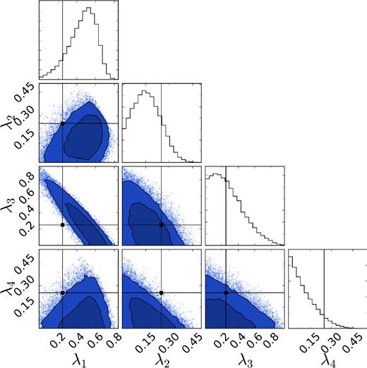
Marginalized 1D and 2D probability density functions for the λ parameters describing the fractional contribution of each of the four subpopulations introduced in Section 2. The thin black lines indicate the true injection fraction from each model, which is 0.25 for all models. The data used were the 80 mock GW events shown in Fig. 2, assumed to have perfect measurements of the spin–orbit misalignment angles cos θ1 and cos θ2. Colours are the same as Fig. 4.
We find that after 80 BBH observations with perfect measurement accuracy, we would be able to confidently establish the presence of all four subpopulations. From this analysis, we can already understand some of the features of the posterior on the hyperparameters. For example, we see that there is a strong degeneracy between λ1 and λ3, since both of these models predict a large (nearly) aligned (θ1 = θ2 = 0) population. There is a similar degeneracy between λ2 and λ4. We can also see that the fraction of exactly aligned systems (λ1) and the fraction of systems with isotropically distributed spin–orbit misalignments (λ2) are not strongly correlated. Both fractions are measured to be between ∼0.15 and ∼0.45 at the 90 per cent credible level with 80 BBH observations, corresponding to a fractional uncertainty of ∼50 per cent.
5.2 Realistic measurement accuracy
We know that in practice GW detectors will not perfectly measure the spin–orbit misalignments of merging BBHs (see Fig. 3 for a typical marginalised posterior). We now use the full set of 80 LALInference posteriors, each containing ∼5000 posterior samples as our input data, when sampling equations (16) and (17).
We show the results of this analysis in Fig. 6. Many of the features seen in the posteriors on the hyperparameters are the same as those seen in Fig. 5, such as the strong anti-correlation between λ1 and λ3. We see that the posterior is not perfectly centred on the true λ values, though the true values do have posterior support. While the hierarchical modelling unambiguously points to the presence of multiple subpopulations, with no single subpopulation able to explain the full set of observations, the data no longer require all four subpopulations to be present.
Marginalized 1D and 2D probability density functions for the λ parameters describing the fractional contribution of each of the four subpopulations introduced in Section 2. The thin black lines indicate the true injection fraction from each model, which is 0.25 for all models. The data used were the full LALInference posteriors of the 80 mock GW events shown in Fig. 2. Colours are the same as Fig. 4.
We have checked that the structure of this posterior is typical given the limited number of observations and the large measurement uncertainties. In the next section, we show that our posteriors converge to the true values in the limit of a large number of detections.
5.3 Dependence on number of observations
The LALInference PE pipeline used to compute the posterior distributions for our 80 injections in Section 3 is computationally expensive. However, we would like to generate a larger catalogue of mock observations. First, this allows us to check that our analysis is self consistent by running many tests, such as confirming that the true result lies within the P per cent credible interval in P per cent of trials. Secondly, it allows us to predict how the accuracy of the inferred fractions of the subpopulations evolves as a function of the number of GW observations.
These posterior models are designed to mimic the typical properties of the posterior on the θ1 and θ2. We have chosen a particular strategy that allows us to make faithful models; starting with models for posteriors on χeff and θ1 before converting them into posteriors on θ1 and θ2 is desirable because χeff and θ1 are only weakly correlated, making it possible to write down independent expressions for the individual likelihoods, while θ1 and θ2 are strongly correlated, so would require a more complex joint likelihood model. The posteriors already implicitly account for marginalization over correlated parameters such as spin magnitudes and the mass ratio, which will not be known in practice. These mock posteriors will not correctly reproduce actual posteriors for specific events, since they do not include the noise realization, except probabilistically; they only reproduce the average properties of the posterior distributions.
We draw ν = 5000 posterior samples of χeff and cos θ1 independently, and calculate the values of cos θ2 using equation (18), fixing the mass ratio q and spin magnitudes χi to their true values. This builds the correct degeneracies between cos θ1 and cos θ2 into the mock posteriors. We show an example of a posterior distribution generated this way in Fig. 7.
Using this method, we generate spin–orbit misalignment posteriors for 400 BBHs drawn in equal fractions (λi = 0.25) from the four subpopulation models introduced in Section 2. Using the method introduced in Section 4, we calculate the posteriors on the λ parameters after 0 (prior), 10, 20, 40, 80, 160 and 400 observations, similar to Mandel et al. (2017). In Fig. 8, we show the 68 per cent and 95 per cent credible intervals for the fraction λ2 of observed BBHs coming from an isotropic distribution (subpopulation 2), corresponding to dynamically formed binaries. Given our models and incorporating realistic measurement uncertainties, we find that this fraction can be measured with a ∼40 per cent fractional uncertainty after 100 observations. Since subpopulations 1 and 3 are somewhat degenerate in our model, we find that the combined fraction λ1 + λ3 is a well-measured parameter (as shown in Fig. 9), whilst the individual components are measured less well. For N ≳100 observations, the uncertainties in the λℓ scale as the inverse square root of the number of observations; e.g. |$\sigma _{\lambda _1 + \lambda _3} \approx 0.8\, N^{-1/2}$|.
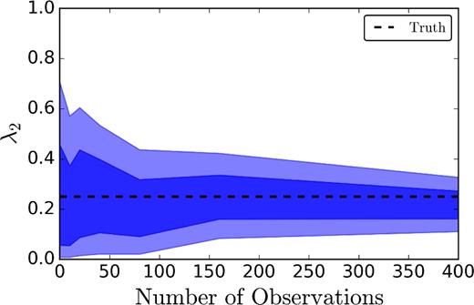
Marginalized posterior on λ2, the fraction of BBHs from the subpopulation with isotropic spin distribution (representing dynamical formation), as a function of the number of GW observations. The posterior converges to the injected value of λ2 = 0.25 (dashed black horizontal line) after ∼100 observations. The coloured bands show the 68 per cent (darkest) and 95 per cent (lightest) credible intervals.
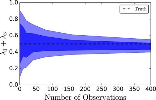
Marginalized posterior on λ1 + λ3, the combined fraction of BBHs formed through subpopulations 1 and 3, as a function of the number of GW observations. These subpopulations correspond to spins preferentially aligned with the orbital angular momentum. The posterior converges to the injected value of λ1 + λ3 = 0.5 (dashed black horizontal line) after ∼20 observations. The coloured bands show the 68 per cent (darkest) and 95 per cent (lightest) credible intervals.
Although ≳ 100 observations are required to accurately measure the contribution of each of the four subpopulations, it is possible to test for more extreme models with fewer observations. For example, ∼20 observations are sufficient to demonstrate the presence of an isotropic subpopulation at the 95 per cent credible level.
Inference using small numbers of observations is sensitive to the exact choice of these observations (both true parameters and measurement errors), which we randomly draw from the relevant distributions. We therefore repeat this test 100 times to account for the random nature of the mock catalogue. In all cases, we find that with only five observations of BBHs with component spin magnitudes χ = 0.7, the exactly aligned model λ1 = 1 can be ruled out at more than 5σ confidence. Similarly, when drawing from the exactly aligned model, we find that the hypothesis that all events come from an isotropic population λ2 = 1 can be ruled out at more than 5σ confidence in all tests with five observations.
6 DISCUSSION AND CONCLUSIONS
With the first direct observations of GWs from merging BBHs, the era of GW astronomy has begun. GW observations provide a new and unique insight into the properties of BBHs and their progenitors. For individual systems, we can infer the masses and spins of the component BHs; combining these measurements we can learn about the population, and place constraints on the formation mechanisms for these systems, whether as the end point of isolated binary evolution or as the results of dynamical interactions.
In this work, we investigated how measurements of BBH spin–orbit misalignments could inform our understanding of the BBH population. We chose the properties of our sources to match those we hope to observe with aLIGO and AdV (at design sensitivity), using four different astrophysically motivated subpopulations for the distribution of spin–orbit misalignment angles, each reflecting a different formation scenario. We performed a Bayesian analysis of GW signals (using full inspiral–merger–ringdown waveforms) for a population of BBHs. We assumed a mixture model for the overall population of BBH spin–orbit misalignments and combined the full PE results from our GW analysis in a hierarchical framework to infer the fraction of the population coming from each subpopulation. A similar analysis could be performed following the detection of real signals.
Adopting a population with spins of χ = 0.7, we demonstrate that the fraction of BBHs with spins preferentially aligned with the orbital angular momentum (λ1 + λ3) is well measured and can be measured with an uncertainty of ∼10 per cent with 100 observations, scaling as the inverse square root of the number of observations. We also show that after 100 observations, we can measure the fraction λ2 of the subpopulation with isotropic spins (assumed to correspond to dynamical formation) with a fractional uncertainty of ∼40 per cent. Extreme hypotheses can be tested and ruled out with even fewer observations. For example, with just five observations, we can rule out the hypothesis that all BBHs have their spins exactly aligned with high confidence (>5σ), if the true population has isotropically distributed spins, and vice versa. This number of observations may be reached by the end of the second aLIGO observing run.
One limitation of the current approach is the assumption that the subpopulation distributions are known perfectly. This will not be the case in practice, but the simplified models considered here are still relevant as parametrizable proxies for astrophysical scenarios. Hierarchical modelling with strong population assumptions could lead to systematic biases in the interpretation of the observations if those assumptions are not representative of the true populations; this can be mitigated by coupling such analysis with weakly modelled approaches, such as observation-based clustering (Mandel et al. 2015, 2017).
In this work we have not taken into account observational selection effects, particularly the differences in the detectabilty of different subpopulations because their different spin parameter distributions impact the SNR (Reisswig et al. 2009). These must be incorporated in the analysis to correctly infer the intrinsic subpopulation fractions (Farr et al., in preparation), but the impact is not expected to be significant in this case. Care must also be taken to avoid biases when performing an hierarchical analysis with real observations, since the observations will not be drawn from the same distribution as the priors used for the analysis of individual events. Our framework accounts for the differences in the priors on the parameters of interest (spin–orbit misalignment angles) between the original PE and model predictions, but not for any discrepancy in the priors of the parameters we marginalize over (e.g. masses); this is likely a second-order effect.
Neither theoretical models nor observations can currently place tight constraints on the spin magnitudes of BHs. We therefore chose to give all BHs a spin magnitude of 0.7 in this study. This choice is clearly ad hoc; we expect a distribution of BH spin magnitudes in nature. Since GW events with BHs with low spin will not constrain the spin–orbit misalignment angles well, a distribution of spin magnitudes containing lower BH spins will act to increase the requirements for the numbers of observations quoted here. Even with significantly smaller BH spin magnitudes, a few to a few tens of observations can distinguish between sufficiently different subpopulation models for spin–orbit misalignment (perfectly aligned versus isotropic) as shown in Farr et al. (2017).
Here, we have assumed that BHs receive large natal kicks, comparable to neutron stars, leading to relatively large spin–orbit misalignments even for isolated binary evolution. We further assume that the effect of the kick is simply to tilt the orbital plane, but not the BH spin. There is, however, evidence from the Galactic double pulsar PSR J0737−3039 that the second born pulsar received a spin tilt at birth (Farr et al. 2011). Furthermore, alignment through mass transfer prior to BH formation may be imperfect. Our models of BBHs that are preferentially but imperfectly aligned because of high natal kicks can be viewed as proxies for misalignment through a combination of these effects.
Optimal hierarchical modelling should fold in all available information, including component masses (cf. Rodriguez et al. 2016) and spin magnitudes (cf. Gerosa & Berti 2017; Fishbach, Holz & Farr 2017), into a single analysis. Complementary electromagnetic observations of high-mass X-ray binaries, Galactic radio pulsars, short gamma-ray bursts, supernovae and luminous red novae will contribute to a concordance model of massive binary formation and evolution.
Acknowledgements
This work was supported in part by the Science and Technology Facilities Council. IM acknowledges support from the Leverhulme Trust. We are grateful for computational resources provided by Cardiff University, and funded by an STFC grant supporting UK Involvement in the Operation of Advanced LIGO. SS and IM acknowledge partial support by the National Science Foundation under Grant No. NSF PHY11-25915. We are grateful to colleagues from the Institute of Gravitational-wave Astronomy at the University of Birmingham, as well as Ben Farr, M. Coleman Miller, Chris Pankow and Salvatore Vitale for fruitful discussions. We thank Davide Gerosa and the anonymous referee for comments on the paper. Corner plots were made using triangle.py available from https://github.com/dfm/triangle.py. This is LIGO Document P1700007.
Throughout this paper, we use geometric units G = c = 1 unless otherwise stated.
A more efficient method of evolving binaries from wide-orbital separations to the frequencies where they enter the aLIGO band was introduced in Kesden et al. (2015) and Gerosa et al. (2015). This exploits the hierarchy of time-scales in the problem and integrates precession averaged equations of motion on the radiation reaction time-scale, rather than integrating the orbit-averaged equations we use here.
These parameters are (e.g. Veitch et al. 2015a) two component masses {mi}; six spin parameters describing |$\lbrace \boldsymbol {S}_i\rbrace$|; two sky coordinates; distance DL; inclination and polarization angles; a reference time, and the orbital phase at this time.
Available as part of the LIGO Scientific Collaboration Algorithm Library (LAL) https://wiki.ligo.org/DASWG/LALSuite.
Non-stationary, non-Gaussian noise has been shown not to affect average PE performance for binary neutron stars (Berry et al. 2015); however, these noise features could be more significant in analysing the shorter duration BBH signals.
Available from http://dan.iel.fm/emcee/.
REFERENCES
