


Abstract
Many high-state non-magnetic cataclysmic variables (CVs) exhibit blueshifted absorption or P-Cygni profiles associated with ultraviolet (UV) resonance lines. These features imply the existence of powerful accretion disc winds in CVs. Here, we use our Monte Carlo ionization and radiative transfer code to investigate whether disc wind models that produce realistic UV line profiles are also likely to generate observationally significant recombination line and continuum emission in the optical waveband. We also test whether outflows may be responsible for the single-peaked emission line profiles often seen in high-state CVs and for the weakness of the Balmer absorption edge (relative to simple models of optically thick accretion discs). We find that a standard disc wind model that is successful in reproducing the UV spectra of CVs also leaves a noticeable imprint on the optical spectrum, particularly for systems viewed at high inclination. The strongest optical wind-formed recombination lines are H α and He ii λ4686. We demonstrate that a higher density outflow model produces all the expected H and He lines and produces a recombination continuum that can fill in the Balmer jump at high inclinations. This model displays reasonable verisimilitude with the optical spectrum of RW Trianguli. No single-peaked emission is seen, although we observe a narrowing of the double-peaked emission lines from the base of the wind. Finally, we show that even denser models can produce a single-peaked H α line. On the basis of our results, we suggest that winds can modify, and perhaps even dominate, the line and continuum emission from CVs.
INTRODUCTION
Cataclysmic variables (CVs) are systems in which a white dwarf (WD) accretes matter from a donor star via Roche lobe overflow. In non-magnetic systems, this accretion is mediated by a Keplerian disc around the WD. Nova-like variables (NLs) are a subclass of CVs in which the disc is always in a relatively high-accretion-rate state (|$\dot{M} \sim 10^{-8}$| M⊙ yr−1). This makes NLs an excellent laboratory for studying the properties of steady-state accretion discs.
It has been known for a long time that winds emanating from the accretion disc are important in shaping the ultraviolet (UV) spectra of high-state CVs (Heap et al. 1978; Greenstein & Oke 1982). The most spectacular evidence for such outflows are the P-Cygni-like profiles seen in UV resonance lines such as C iv λ1550 (see e.g. Cordova & Mason 1982). Considerable effort has been spent over the years on understanding and modelling these UV features (e.g. Drew & Verbunt 1985; Drew 1987; Mauche & Raymond 1987; Shlosman & Vitello 1993 [hereafter SV93]; Knigge, Woods & Drew 1995; Knigge & Drew 1997; Knigge et al. 1997; Long & Knigge 2002 [hereafter LK02]; Noebauer et al. 2010; Puebla et al. 2011). The basic picture emerging from these efforts is of a slowly accelerating, moderately collimated bipolar outflow that carries away ≃ 1–10 per cent of the accreting material. State-of-the-art simulations of line formation in this type of disc wind can produce UV line profiles that are remarkably similar to observations.
Much less is known about the effect of these outflows on the optical spectra of high-state CVs. These spectra are typically characterized by H and He emission lines superposed on a blue continuum. In many cases, and particularly in the SW Sex subclass of NLs (Honeycutt et al. 1986; Dhillon & Rutten 1995), these lines are single peaked. This is contrary to theoretical expectations for lines formed in accretion discs, which are predicted to be double peaked (Smak 1981; Horne & Marsh 1986). Low-state CVs (dwarf novae in quiescence) do, in fact, exhibit such double-peaked lines (Marsh & Horne 1990).
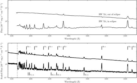
Murray & Chiang (1996, 1997, hereafter referred to collectively as MC96) have shown that the presence of disc winds may offer a natural explanation for the single-peaked optical emission lines in high-state CVs, since they can strongly affect the radiative transfer of line photons. Strong support for a significant wind contribution to the optical emission lines comes from observations of eclipsing systems. There, the single-peaked lines are often only weakly eclipsed, and a significant fraction of the line flux remains visible even near mid-eclipse (e.g. Baptista et al. 2000; Groot, Rutten & van Paradijs 2004). This points to line formation in a spatially extended region, such as a disc wind (see Fig. 1). Further evidence for a wind contribution to the optical lines comes from isolated observations of P-Cygni-like line profiles even in optical lines, such as H α and He i λ5876 (Patterson et al. 1996; Ringwald & Naylor 1998; Kafka & Honeycutt 2004).
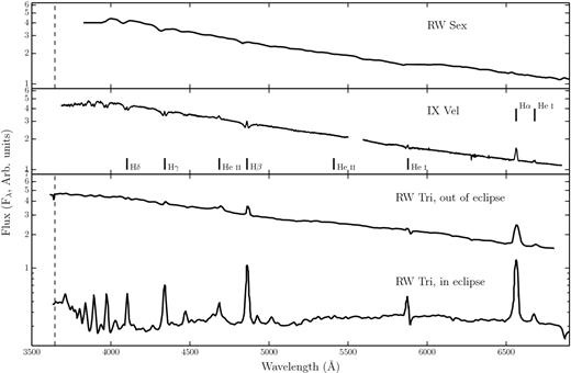
Optical spectra of three NLs: RW Sex (top; Beuermann, Stasiewski & Schwope 1992), IX Vel (top middle; Pala & Gaensicke, private communication) and RW Tri in and out of eclipse (bottom two panels; Groot et al. 2004). The data for RW Sex and RW Tri were digitized from the respective publications, and the IX Vel spectrum was obtained using the XSHOOTER spectrograph on the Very Large Telescope on 2014 October 10. These systems have approximate inclinations of 30°, 60° and 80° (see Section 5.4), respectively. The trend of increasing Balmer line emission with inclination can be seen. In RW Tri strong single-peaked emission in the Balmer lines is seen even in eclipse, indicating that the lines may be formed in a spatially extensive disc wind, and there is even a suggestion of a (potentially wind-formed) recombination continuum in the eclipsed spectrum. We have attempted to show each spectrum over a similar dynamic range.
Could disc winds also have an impact on the UV/optical continuum of high-state CVs? This continuum is usually thought to be dominated by the accretion disc and modelled by splitting the disc into a set of concentric, optically thick, non-interacting annuli following the standard Teff(R)∝R−3/4 radial temperature distribution (Shakura & Sunyaev 1973). In such models, each annulus is taken to emit either as a blackbody or, perhaps more realistically, as a stellar/disc atmosphere model (Schwarzenberg-Czerny & Rózyczka 1977; Wade 1984, 1988). In the latter case, the local surface gravity, log g(R), is assumed to be set solely by the accreting WD, since self-gravity is negligible in CV discs.
Attempts to fit the observed spectral energy distributions (SEDs) of high-state CVs with such models have met with mixed success. In particular, the SEDs predicted by most stellar/disc atmosphere models are too blue in the UV (Wade 1988; Long et al. 1991, 1994; Knigge et al. 1998) and exhibit stronger-than-observed Balmer jumps in absorption (Wade 1984; Haug 1987; La Dous 1989b; Knigge et al. 1998). One possible explanation for these problems is that these models fail to capture all of the relevant physics. Indeed, it has been argued that a self-consistent treatment can produce better agreement with observational data (e.g. Shaviv & Wehrse 1991; but see also Idan et al. 2010). However, an alternative explanation, suggested by Knigge et al. (1998; see also Hassall 1985), is that recombination continuum emission from the base of the disc wind might fill in the disc's Balmer absorption edge and flatten the UV spectrum.
Here, we carry out Monte Carlo radiative transfer simulations in order to assess the likely impact of accretion disc winds on the optical spectra of high-state CVs. More specifically, our goal is to test whether disc winds of the type developed to account for the UV resonance lines would also naturally produce significant amounts of optical line and/or continuum emission. In order to achieve this, we have implemented the ‘macro-atom’ approach developed by Lucy (2002, 2003) into the Monte Carlo ionization and radiative transfer code described by LK02 (a process initiated by Sim, Drew & Long 2005, hereafter SDL05). With this upgrade, the code is able to deal correctly with processes involving excited levels, such as the recombination emission produced by CV winds.
The remainder of this paper is organized as follows. In Section 2, we briefly describe the code and the newly implemented macro-atom approach. In Section 3, we describe the kinematics and geometry of our disc wind model. In Section 4, we present spectra simulated from the benchmark model employed by LK02, and, in Section 5, we present a revised model optimized for the optical waveband. In Section 6, we summarize our findings.
python: A MONTE CARLO IONIZATION AND RADIATIVE TRANSFER CODE
python is a Monte Carlo ionization and radiative transfer code which uses the Sobolev approximation to treat line transfer (e.g. Sobolev 1957, 1960; Rybicki & Hummer 1978). The code has already been described extensively by LK02, SDL05 and Higginbottom et al. (2013, hereafter H13), so here we provide only a brief summary of its operation, focusing particularly on new aspects of our implementation of macro-atoms into the code.
Basics
python operates in two distinct stages. First, the ionization state, level populations and temperature structure are calculated. This is done iteratively, by propagating several populations of Monte Carlo energy quanta (‘photons’) through a model wind. The geometric and kinematic properties of the outflow are specified on a pre-defined spatial grid. In each of these iterations (‘ionization cycles’), the code records estimators that characterize the radiation field in each grid cell. At the end of each ionization cycle, a new electron temperature is calculated that more closely balances heating and cooling in the plasma. The radiative estimators and updated electron temperature are then used to revise the ionization state of the wind, and a new ionization cycle is started. The process is repeated until heating and cooling are balanced throughout the wind.
This converged model is then used as the basis for the second set of iterations (‘spectral cycles’). In these, the emergent spectrum over the desired spectral range is synthesized by tracking populations of energy packets through the wind and computing the emergent spectra at a number of user-specified viewing angles.
python is designed to operate in a number of different regimes, both in terms of the scale of the system and in terms of the characteristics of the underlying radiation field. It was originally developed by LK02 in order to model the UV spectra of CVs with a simple biconical disc wind model. SDL05 used the code to model Brackett and Pfund line profiles of H in young-stellar objects (YSOs). As part of this effort, they implemented a ‘macro-atom’ mode (see below) in order to correctly treat H recombination lines with python. Finally, H13 used python to model broad absorption line QSOs. For this application, an improved treatment of ionization was implemented, so that the code is now capable of dealing with arbitrary photoionizing SEDs, including non-thermal and multicomponent ones.
Ionization and excitation: ‘simple atoms’
Finally, python originally modelled all bound–bound processes as transitions within a simple two-level atom (e.g. Mihalas 1982). This framework was used for the treatment of line transfer and also for the line heating and cooling calculations (see LK02). The approximation works reasonably well for resonance lines, such as C iv λ1550, in which the lower level is the ground state. However, it is a poor approximation for many other transitions, particularly those where the upper level is primarily populated from above. Thus an improved method for estimating excited level populations and simulating line transfer is needed in order to model recombination lines and continua.
Ionization and excitation: macro-atoms
Lucy (2002, 2003, hereafter L02, L03, respectively) has shown that it is possible to calculate the emissivity of a gas in statistical equilibrium accurately by quantising matter into ‘macro-atoms’, and radiant and kinetic energy into indivisible energy packets (r- and k- packets, respectively). His macro-atom scheme allows for all possible transition paths from a given level and provides a full non-local thermodynamic equilibrium (NLTE) solution for the level populations based on Monte Carlo estimators. The macro-atom technique has already been used to model Wolf–Rayet star winds (Sim 2004), AGN disc winds (Sim et al. 2008; Tatum et al. 2012), supernovae (Kromer & Sim 2009; Kerzendorf & Sim 2014) and YSOs (SDL05). A full description of the approach can be found in L02 and L03.
Ionization and excitation: a hybrid approach
SDL05 implemented a macro-atom treatment of H in python and used this to predict the observable properties of a pure H wind model for YSOs. Our goal here is to simultaneously model the optical and UV spectra of high-state CVs. Since the optical spectra are dominated by H and He recombination lines, both of these species need to be treated as macro-atoms. The UV spectra, on the other hand, are dominated by resonance lines associated with metals. This means we need to include these species in our models, but they can be treated with our (much faster) simple-atom approach. We have therefore implemented a hybrid ionization and excitation scheme into python. Any atomic species can now be treated either in our simple-atom approximation or with the full macro-atom machinery. In our CV models, we treat H and He as macro-atoms and all metals as simple-atoms. Species treated with either method are fully taken into account as sources of both bound–free opacity and line opacity, and contribute to the heating and cooling balance of the plasma.
Atomic data
We generally use the same atomic data as H13, which is an updated version of that described by LK02. In addition, we follow SDL05 in treating H as a 20-level atom, where each level is defined by the principal quantum number, n. For the macro-atom treatment of He, we have added the additional level and line information required from topbase (Badnell et al. 2005). He ii is treated in much the same way as H, but with 10 levels. He i has larger energy differentials between different l-subshells and triplet and singlet states. Thus, we still include levels up to n = 10, but explicitly treat the l and s sub-orbitals as distinct levels instead of assuming they are perfectly ‘l-mixed’. This allows us to model the singlet and triplet He i lines that are ubiquitous in the optical spectra of CVs (e.g. Dhillon 1996).
Code validation and testing
python has been tested against a number of radiative transfer and photoionization codes. LK02 and H13 conducted comparisons of ionization balance with cloudy (Ferland et al. 2013), demonstrating excellent agreement. We have also carried out comparisons of ionization and spectral synthesis with the supernova code tardis.tardis is described by Kerzendorf & Sim (2014), and the spectral comparisons can be found therein. For the effort reported here, we have additionally carried out tests of the macro-atom scheme in python. Fig. 2 shows two of these tests. In the top panel, we compare the Balmer series emissivities as predicted by python in the l-mixed Case B limit against the analytical calculations by Seaton (1959). In the bottom panel, we compare python and tardis predictions of He i level populations for a particular test case. Agreement is excellent for both H and He.
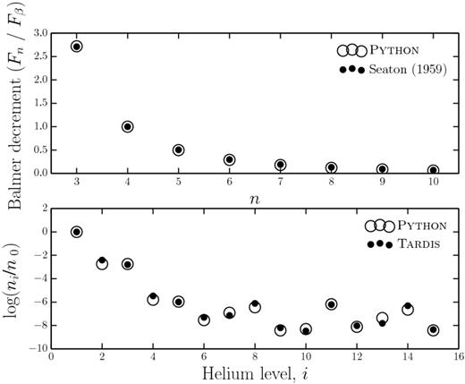
Top panel: ‘Case B’ Balmer decrements computed with python compared to analytic calculations by Seaton (1959). Both calculations are calculated at Te = 10 000 K (see Osterbrock 1989 for a discussion of this commonly used approximation). Bottom panel: a comparison of He i level populations (the most complex ion we currently treat as a macro-atom) between python and tardis models. The calculation is conducted with physical parameters of ne = 5.96 × 104 cm−3, Te = 30 600 K, TR = 43 482 K and W = 9.65 × 10⁻⁵. Considering the two codes use different atomic data and tardis, unlike python, currently has a complete treatment of collisions between radiatively forbidden transitions, the factor of <2 agreement is encouraging.
DESCRIBING THE SYSTEM AND ITS OUTFLOW
python includes several different kinematic models of accretion disc winds, as well as different options for describing the physical and radiative properties of the wind-driving system under consideration. Most of these features have already been discussed by LK02 and H13, so below we only briefly recount the key aspects of the particular system and wind model used in the present study.
Wind geometry and kinematics
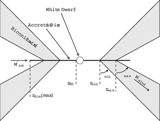
Cartoon illustrating the geometry and kinematics of the benchmark CV wind model.
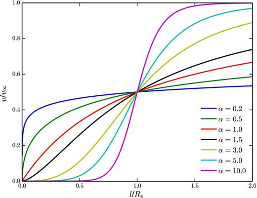
The adopted poloidal velocity law for various values of the acceleration exponent, α.
Sources and sinks of radiation
The net photon sources in our CV model are the accretion disc, the WD and, in principle, a boundary layer with user-defined temperature and luminosity. All of these radiating bodies are taken to be optically thick, and photons striking them are assumed to be destroyed instantaneously. The secondary star is not included as a radiation source, but is included as an occulting body. This allows us to model eclipses. Finally, emission from the wind itself is also accounted for, but note that we assume the outflow to be in radiative equilibrium. Thus all of the heating of the wind, as well as its emission, is ultimately powered by the radiation field of the net photon sources in the simulation. In the following sections, we will describe our treatment of these system components in slightly more detail.
Accretion disc
python has some flexibility when treating the accretion disc as a source of photons. The disc is broken down into annuli such that each annulus contributes an equal amount to the bolometric luminosity. We take the disc to be geometrically thin, but optically thick, and thus adopt the temperature profile of a standard Shakura & Sunyaev (1973) α-disc. An annulus can then be treated either as a blackbody with the corresponding effective temperature or as a stellar atmosphere model with the appropriate surface gravity and effective temperature. Here, we use blackbodies during the ionization cycles and to compute our Monte Carlo estimators. However, during the spectral synthesis stage of the simulation we use stellar atmosphere models. This produces more realistic model spectra and allows us to test if recombination emission from the wind base can fill in the Balmer jump, which is always in absorption in these models. Our synthetic stellar atmosphere spectra are calculated with synspec1 from either Kurucz (Kurucz 1991) atmospheres (for Teff ≤ 50 000 K) or from tlusty (Hubeny & Lanz 1995) models (for Teff > 50 000 K).
White dwarf
The WD at the centre of the disc is always present as a spherical occulting body with radius RWD in python CV models, but it can also be included as a source of radiation. In the models presented here, we treat the WD as a blackbody radiator with temperature TWD and luminosity |$L_{\rm WD} = 4\pi R_{\rm WD}^2 \sigma T_{\rm WD}^4$|.
Boundary layer
It is possible to include radiation from a boundary layer (BL) between the disc and the WD. In python, the BL is described as a blackbody with a user-specified effective temperature and luminosity. In the models presented here, we have followed LK02 in setting the BL luminosity to zero. However, we have confirmed that the addition of an isotropic BL with LBL = 0.5Lacc and temperatures in the range 80 kK ≤ TBL ≤ 200 kK would not change any of our main conclusions.
Secondary star
The donor star is included in the system as a pure radiation sink, i.e. it does not emit photons, but absorbs any photons that strike its surface. The secondary is assumed to be Roche lobe filling, so its shape and relative size are defined by setting the mass ratio of the system, q = M2/MWD. The inclusion of the donor star as an occulting body allows us to model eclipses of the disc and the wind. For this purpose, we assume a circular orbit with a semimajor axis a and specify orbital phase such that Φorb = 0 is the inferior conjunction of the secondary (i.e. mid-eclipse for i ≃ 90°).
A BENCHMARK DISC WIND MODEL
Our main goal is to test whether the type of disc wind model that has been successful in explaining the UV spectra of CVs could also have a significant impact on the optical continuum and emission line spectra of these systems. In order to set a benchmark, we therefore begin by investigating one of the fiducial CV wind models that was used by SV93 and LK02 to simulate the UV spectrum of a typical high-state system. The specific parameters for this model (model A) are listed in Table 1. A key point is that the wind mass-loss rate in this model is set to 10 per cent of the accretion rate through the disc. We follow SV93 in setting the inner edge of the wind (rmin) to 4 RWD. The sensitivity to some of these parameters is briefly discussed in Section 5.
Parameters used for the geometry and kinematics of the benchmark CV model (model A), which is optimized for the UV band, and a model which is optimized for the optical band and described in Section 5 (model B). For model B, only parameters which are altered are given – otherwise the model A parameter is used. Porb is the orbital period (the value for RW Tri from Walker 1963 is adopted, see Section 5.4) and R2 is the radius of a sphere with the volume of the secondary's Roche lobe. Other quantities are defined in the text or Fig. 3. Secondary star parameters are only quoted for model B as we do not show eclipses with the benchmark model (see Section 5.4).
| Model parameters | ||
|---|---|---|
| Parameter | Model A | Model B |
| MWD | 0.8 M⊙ | |
| RWD | 7 × 108 cm | |
| TWD | 40 000 K | |
| M2 | - | 0.6 M⊙ |
| q | - | 0.75 |
| Porb | - | 5.57 h |
| a | - | 194.4 RWD |
| R2 | - | 69.0 RWD |
| |$\dot{M}_{\rm acc}$| | 10−8 M⊙ yr−1 | |
| |$\dot{M}_{\rm wind}$| | 10−9 M⊙ yr−1 | |
| rmin | 4 RWD | |
| rmax | 12 RWD | |
| rdisc(max) | 34.3 RWD | |
| θmin | 20° | |
| θmax | 65° | |
| γ | 1 | |
| v∞ | 3 vesc | |
| Rv | 100 RWD | 142.9 RWD |
| α | 1.5 | 4 |
Physical structure and ionization state
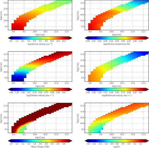
The physical properties of the wind – note the logarithmic scale. Near the disc plane the wind is dense, with low poloidal velocities. As the wind accelerates it becomes less dense and more highly ionized. The dominant He ion is almost always He iii, apart from in a small portion of the wind at the base, which is partially shielded from the inner disc.
There is an obvious drop-off in density and temperature with distance away from the disc, so any line formation process that scales as ρ2 – i.e. recombination and collisionally excited emission – should be expected to operate primarily in the dense base of the outflow. Moreover, a comparison of the rotational and poloidal velocity fields shows that rotation dominates in the near-disc regime, while outflow dominates further out in the wind.
The ionization equation used in the ‘simple atom’ approach used by LK02 (see Section 2.2) should be a reasonable approximation to the photoionization equilibrium in the benchmark wind model. Even though the macro-atom treatment of H and He does affect the computation of the overall ionization equilibrium, we would expect the resulting ionization state of the wind to be quite similar to that found by LK02. The bottom panels in Fig. 5 confirm that this is the case. In particular, He is fully ionized throughout most of the outflow, except for a small region near the base of the wind, which is shielded from the photons produced by the hot inner disc. In line with the results of LK02, we also find that Civ is the dominant C ion throughout the wind, resulting in a substantial absorbing column across a large range of velocities. As we shall see, this produces the broad, deep and blueshifted Civ λ1550 absorption line that is usually the most prominent wind-formed feature in the UV spectra of low-inclination nova-like CVs.
Synthetic spectra
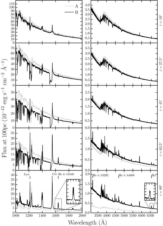
We begin by verifying that the benchmark model still produces UV spectra that resemble those observed in CVs. We do expect this to be the case, since the ionization state of the wind has not changed significantly from that computed by LK02 (see Section 4.1). The left column of panels in Fig. 6 shows that this expectation is met: all of the strong metal resonance lines – notably N v λ1240, Si iv λ1400 and C iv λ1550 – are present and exhibit clear P-Cygni profiles at intermediate inclinations. In addition, however, we now also find that the wind produces significant Ly α and He ii λ1640 emission lines.
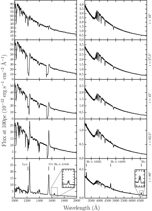
UV (left) and optical (right) synthetic spectra for model A, our benchmark model, computed at sightlines of 10°, 27| $_{.}^{\circ}$|5, 45°, 62| $_{.}^{\circ}$|5 and 80°. The inset plots show zoomed-in line profiles for He ii λ1640 and H α. Double-peaked line emission can be seen in He ii λ1640, He ii λ4686, H α and some He i lines, but the line emission is not always sufficient to overcome the absorption cores from the stellar atmosphere models. The model also produces a prominent He ii λ3202 line at high inclinations.
Fig. 6 (right-hand panel) and Fig. 7 show the corresponding optical spectra produced for the benchmark model, and these do exhibit some emission lines associated with H and He. We see a general trend from absorption lines to emission lines with increasing inclination, as one might expect from our wind geometry. This trend is consistent with observations, as can be seen in Fig. 1. However, it is clear that this particular model does not produce all of the lines seen in observations of high-state CVs. The higher order Balmer series lines are too weak to overcome the intrinsic absorption from the disc atmosphere, and the wind fails to produce any observable emission at low and intermediate inclinations. This contrasts with the fact that emission lines are seen in the optical spectra of (for example) V3885 Sgr (Hartley et al. 2005) and IX Vel (Beuermann & Thomas 1990, see also fig. 1).
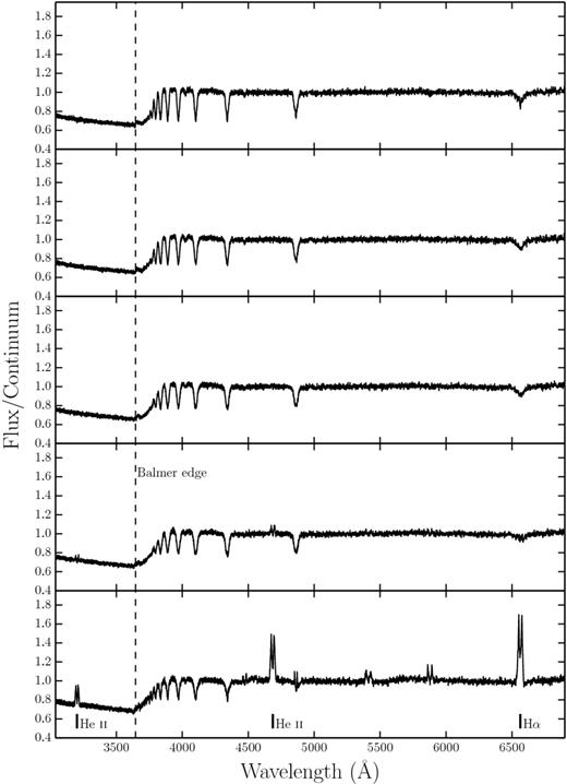
Synthetic optical spectra from model A computed for sightlines of 10°, 27| $_{.}^{\circ}$|5, 45°, 62| $_{.}^{\circ}$|5 and 80°. In these plots the flux is divided by a polynomial fit to the underlying continuum redwards of the Balmer edge, so that line-to-continuum ratios and the true depth of the Balmer jump can be shown.
The emissivity of these recombination features scales as ρ2, meaning that they form almost entirely in the dense base of the wind, just above the accretion disc. Here, the velocity field of the wind is still dominated by rotation, rather than outflow, which accounts for the double-peaked shape of the lines. In principle, lines formed in this region can still be single peaked, since the existence of a poloidal velocity gradient changes the local escape probabilities (MC96). However, as discussed further in Section 5.3, the radial velocity shear in our models is not high enough for this radiative transfer effect to dominate the line shapes.
The Balmer jump is in absorption at all inclinations for our benchmark model. This is due to the stellar atmospheres we have used to model the disc spectrum; it is not a result of photoabsorption in the wind. In fact, the wind spectrum exhibits the Balmer jump in emission, but this is not strong enough to overcome the intrinsic absorption edge in the disc spectrum. This is illustrated in Fig. 8, which shows the angle-integrated spectrum of the system, i.e. the spectrum formed by all escaping photons, separated into the disc and wind contributions. Even though the wind-formed Balmer recombination continuum does not completely fill in the Balmer absorption edge in this model, it does already contribute significantly to the total spectrum. This suggests that modest changes to the outflow kinematics might boost the wind continuum and produce emergent spectra with weak or absent Balmer absorption edges.
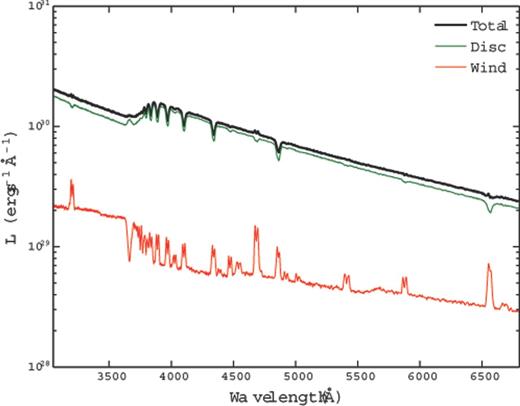
Total packet-binned spectra across all viewing angles, in units of monochromatic luminosity. The thick black line shows the total integrated escaping spectrum, while the green line shows disc photons which escape without being reprocessed by the wind. The red line shows the contributions from reprocessed photons. Recombination continuum emission bluewards of the Balmer edge is already prominent relative to other wind continuum processes, but is not sufficient to fill in the Balmer jump in this specific model
A REVISED MODEL OPTIMIZED FOR OPTICAL WAVELENGTHS
The benchmark model discussed in Section 4 was originally designed to reproduce the wind-formed lines seen in the UV spectra of high-state CVs. As we have seen, this model does produce some observable optical emission. We can now attempt to construct a model that more closely matches the observed optical spectra of CVs.
Specifically, we aim to assess whether a revised model can:
account for all of the lines we see in optical spectra of CVs while preserving the UV behaviour;
produce single-peaked Balmer emission lines;
generate enough of a wind-formed recombination continuum to completely fill in the disc's Balmer absorption edge for reasonable outflow parameters.
The emission measure of a plasma is directly proportional to its density. The simplest way to simultaneously affect the density in the wind (for fixed mass-loss rate), as well as the velocity gradients, is by modifying the poloidal velocity law. Therefore, we focus on just two kinematic variables (Section 3.1):
the acceleration length, Rv, which controls the distance over which the wind accelerates to |$\frac{1}{2} v_{\infty }$|;
the acceleration exponent, α, which controls the rate at which the poloidal velocity changes near Rv.
The general behaviour we might expect is that outflows with denser regions near the wind base – i.e. winds with larger Rv and/or larger α – will produce stronger optical emission signatures. However, this behaviour may be moderated by the effect of the increasing optical depth through this region, which can also affect the line profile shapes. In addition, modifying Rv also increases the emission volume. Based on a preliminary exploration of models with different kinematics, we adopt the parameters listed in table 1 for our ‘optically optimized’ model (model B).
Synthetic spectra
Fig. 9 shows the UV and optical spectra for the optically optimized model for the full range of inclinations. As expected, the trend from absorption to emission in the optical is again present, but in this revised model we produce emission lines in the entire Balmer series at high inclinations, as well as the observed lines in He ii and He i. This can be seen more clearly in the continuum-normalized spectrum in Fig. 10.
UV (left) and optical (right) synthetic spectra for model B computed at sightlines of 10°, 27| $_{.}^{\circ}$|5, 45°, 62| $_{.}^{\circ}$|5 and 80°. Model A is shown in grey for comparison. The inset plots show zoomed-in line profiles for He ii λ1640 and H α. The Balmer and He are double-peaked, albeit with narrower profiles. Strong He ii λ4686 emission can be seen, as well as a trend of a deeper Balmer jump with decreasing inclination.
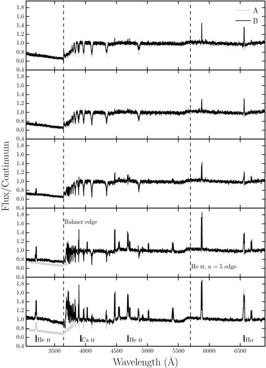
Synthetic optical spectra from model B computed for sightlines of 10°, 27| $_{.}^{\circ}$|5, 45°, 62| $_{.}^{\circ}$|5 and 80°. Model A is shown in grey for comparison. In these plots, the flux is divided by a polynomial fit to the underlying continuum redwards of the Balmer edge, so that line-to-continuum ratios and the true depth of the Balmer jump can be shown.
Two other features are worth noting in the optical spectrum. First, the collisionally excited Ca ii emission line at 3934 Å becomes quite prominent in our densest models. Secondly, our model predicts a detectable He ii recombination line at 3202 Å. This is the He equivalent of Paschen β and should be expected in all systems that feature a strong He ii λ4686 line (the He equivalent of Paschen α). This line is somewhat unfamiliar observationally, because it lies bluewards of the atmospheric cut-off, but also redwards of most UV spectra.
Our models do not exhibit P-Cygni profiles in the optical lines. This is perhaps not surprising. LK02 and SV93 originally designed such models to reproduce the UV line profiles. Thus, most of the wind has an ionization parameter of log U ∼ 2 (see Fig. 5). This means H and He are fully ionized throughout much of the wind and are successful in producing recombination features. However, the line opacity throughout the wind is too low to produce noticeable blue shifted absorption. We suspect that the systems that exhibit such profiles must possess a higher degree of ionization stratification, although the lack of contemporary observations means it is not known for certain if the P-Cygni profiles in UV resonance lines and optical H and He lines exist simultaneously. Ionization stratification could be caused by a clumpy flow, in which the ionization state changes due to small-scale density fluctuations, or a stratification in density and ionizing radiation field over larger scales. Invoking clumpiness in these outflows is not an unreasonable hypothesis. Theories of line-driven winds predict an unstable flow (MacGregor, Hartmann & Raymond 1979; Owocki & Rybicki 1984, 1985), and simulations of CV disc winds also produce density inhomogeneities (Proga, Stone & Drew 1998; Proga et al. 2002). Tentative evidence for clumping being directly related to P-Cygni optical lines comes from the fact that Prinja et al. (2000) found the dwarf nova BZ Cam's outflow to be unsteady and highly mass-loaded in outburst, based on observations of the UV resonance lines. This system has also exhibited P-Cygni profiles in He i λ5876 and H α when in a high state (Patterson et al. 1996; Ringwald & Naylor 1998). The degree of ionization and density variation and subsequent line opacities may be affected by our model parameters and the specific parametrization we have adopted.
In the UV, the model still produces all the observed lines, and deep P-Cygni profiles are produced in the normal resonance lines, as discussed in Section 4.2. However, the UV spectra also display what is perhaps the biggest problem with this revised model, namely the strength of resonance line emission at low and intermediate inclinations. In order to generate strong optical wind signatures, we have adopted wind parameters that lead to very high densities at the base of the wind (ne ∼ 1013–1014 cm−3). This produces the desired optical recombination emission, but also increases the role of collisional excitation in the formation of the UV resonance lines. This explains the pronounced increase in the emission component of the Civ λ1550 resonance line, for example, relative to what was seen in the benchmark model (compare Figs 6 and 9). The strength of this component in the revised model is probably somewhat too high to be consistent with UV observations of high-state CVs (see e.g. Long et al. 1991, 1994; Noebauer et al. 2010).
Continuum shape and the Balmer jump
The wind now also has a clear effect on the continuum shape, as shown by Fig. 11. In fact, the majority of the escaping spectrum has been reprocessed in some way by the wind, either by electron scattering (the wind is now moderately Thomson-thick), or by bound–free processes. This is demonstrated by the flatter spectral shape and the slight He photoabsorption edge present in the optical spectrum (marked in Fig. 10). This reprocessing is also responsible for the change in continuum level between models A and B. In addition, Figs 9, 10 and 11 clearly demonstrate that the wind produces a recombination continuum sufficient to completely fill in the Balmer jump at high inclinations.2 This might suggest that Balmer continuum emission from a wind can be important in shaping the Balmer jump region, as originally suggested by Knigge et al. (1998; see also Hassall 1985).
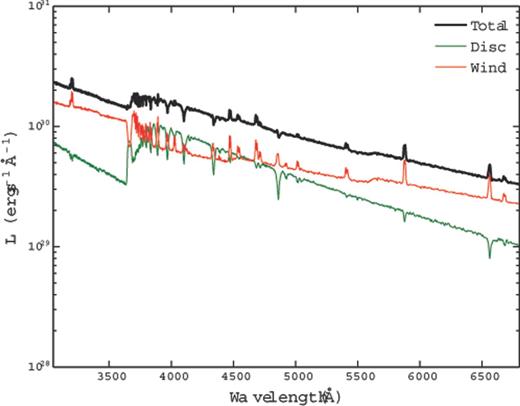
Total packet-binned spectra across all viewing angles, in units of monochromatic luminosity. The thick black line shows the total integrated escaping spectrum, while the green line shows disc photons which escape without being reprocessed by the wind. The red line show the contributions from reprocessed photons. In this denser model the reprocessed contribution is significant compared to the escaping disc spectrum. The Balmer continuum emission is prominent, and the wind has a clear effect on the overall spectral shape.
It should be acknowledged, however, that the Balmer jump in high-state CVs would naturally weaken at high inclinations due to limb-darkening effects (La Dous 1989a, 1989b). Although we include a simple limb-darkening law which affects the emergent flux at each inclination, we do not include it as a frequency-dependent opacity in our model. As a result, the efficiency of filling in the Balmer jump should really be judged at low and medium inclinations, where, although prominent, the recombination continuum does not overcome the disc atmosphere absorption. In addition, this effect could mean that any model which successfully fills in the jump at low inclinations could lead to a Balmer jump in emission at high inclinations. In any case, to properly understand this phenomenon, a fully self-consistent radiative transfer calculation of both the disc atmosphere and connected wind is required.
Line profile shapes: producing single-peaked emission
Fig. 12 shows how the H α profile changes with the kinematics of the wind for an inclination of 80°. The main prediction is that dense, slowly accelerating wind models produce narrower emission lines. This is not due to radial velocity shear. As stated by MC96, that mechanism can only work if poloidal and rotational velocity gradients satisfy (dvl/dr)/(dvϕ/dr) ≳ 1; in our models, this ratio is always ≲ 0.1. Instead, the narrow lines predicted by our denser wind models can be traced to the base of the outflow becoming optically thick in the continuum, such that the line emission from the base of the wind cannot escape to the observer. In such models, the ‘line photosphere’ (the τ ≃ 1 surface of the line-forming region) moves outwards, towards larger vertical and cylindrical distances. This reduces the predicted line widths, since the rotational velocities – which normally provide the main line broadening mechanism at high inclination – drop off as 1/r. This is not to say that the MC96 mechanism could not be at work in CV winds. For example, it would be worth investigating alternative prescriptions for the wind velocity field, as well as the possibility that the outflows may be clumped. An inhomogeneous flow (which has been predicted in CVs; see Section 5.2) might allow large radial velocity shears to exist while still maintaining the high densities needed to produce the required level of emission. However, such an investigation is beyond the scope of this paper.
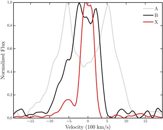
H α line profiles, normalized to 1, plotted in velocity space for three models with varying kinematic properties, computed at an inclination of 80°. The benchmark model and the improved optical model described in Section 6 are labelled as A and B, respectively, and a third model (X) which has an increased acceleration length of Rv = 283.8RWD, and α = 4 is also shown. The x-axis limits correspond to the Keplerian velocity at 4RWD, the inner edge of the wind. We observe a narrowing of the lines, and a single-peaked line in model X. This is not due to radial velocity shear (see Section 5.3).
In our models, single-peaked line profiles are produced once the line-forming region has been pushed up to ∼1011 cm (∼150RWD) above the disc plane. This number may seem unrealistically large, but the vertical extent of the emission region is actually not well constrained observationally. In fact, multiple observations of eclipsing NLs show that the H α line is only moderately eclipsed compared to the continuum (e.g. Baptista et al. 2000; Groot et al. 2004; see also Section 5.4), implying a significant vertical extent for the line-forming region. This type of model should therefore not be ruled out a priori, but this specific model was not adopted as our optically optimized model due to its unrealistically high continuum level in eclipse.
Sensitivity to model parameters
This revised model demonstrates that one can achieve a more realistic optical spectrum by altering just two kinematic parameters. However, it may also be possible to achieve this by modifying other free parameters such as |$\dot{M}_{\rm wind}$|, the opening angles of the wind and the inner and outer launch radii. For example, increasing the mass-loss rate of the wind increases the amount of recombination emission (which scales as ρ2), as well as lowering the ionization parameter and increasing the optical depth through the wind. Larger launching regions and covering factors tend to lead to a larger emitting volume, but this is moderated by a decrease in density for a fixed mass-loss rate. We also note that the inner radius of 4RWD adopted by SV93 affects the emergent UV spectrum seen at inclinations <θmin as the inner disc is uncovered. This causes less absorption in the UV resonance lines, but the effect on the optical spectrum is negligible. We have verified this general behaviour, but we suggest that future work should investigate the effect of these parameters in more detail, as well as incorporating a treatment of clumping. If a wind really does produce the line and continuum emission seen in optical spectra of high-state CVs, then understanding the true mass-loss rate and geometry of the outflow is clearly important.
Comparison to RW Tri
Fig. 13 shows a comparison of the predicted out-of-eclipse and mid-eclipse spectra against observations of the high-inclination nova-like RW Tri. The inclination of RW Tri is somewhat uncertain, with estimates including 70| $_{.}^{\circ}$|5 (Smak 1995), 75° (Groot et al. 2004), 80° (Longmore et al. 1981) and 82°(Frank & King 1981). Here, we adopt i = 80°, but our qualitative conclusions are not particularly sensitive to this choice. We follow LK02 is setting the value of rdisc (the maximum radius of the accretion disc) to 34.3RWD. When compared to the semimajor axis of RW Tri, this value is perhaps lower than one might typically expect for NLs (Harrop-Allin & Warner 1996). However, it is consistent with values inferred by Rutten, van Paradijs & Tinbergen (1992). We emphasize that this model is in no sense a fit to this – or any other – data set.
Top panel: in and out of eclipse spectra of the high-inclination NL RW Tri. Bottom panel: in and out of eclipse synthetic spectra from model B. The artificial ‘absorption’ feature just redwards of the Balmer jump is caused for the reasons described in Section 5.2.
The similarity between the synthetic and observed spectra is striking. In particular, the revised model produces strong emission in all the Balmer lines, with line-to-continuum ratios comparable to those seen in RW Tri. Moreover, the line-to-continuum contrast increases during eclipse, as expected for emission produced in a disc wind. This trend is in line with the observations of RW Tri, and it has also been seen in other NLs, including members of the SW Sex class (Neustroev et al. 2011). As noted in Section 5.2, the majority of the escaping radiation has been reprocessed by the wind in some way (particularly the eclipsed light).
However, there are also interesting differences between the revised model and the RW Tri data set. For example, the model exhibits considerably stronger He ii features than the observations, which suggests that the overall ionization state of the model is somewhat too high. As discussed in Section 5.3, the optical lines are narrow, but double peaked. This is in contrast to what is generally seen in observations of NLs, although the relatively low resolution of the RW Tri spectrum makes a specific comparison difficult. In order to demonstrate the double-peaked nature of the narrower lines, we choose not to smooth the synthesized data to the resolution of the RW Tri data set. If the data were smoothed, the H α line would appear single peaked.
CONCLUSIONS
We have investigated whether a disc wind model designed to reproduce the UV spectra of high-state CVs would also have a significant effect on the optical spectra of these systems. We find that this is indeed the case. In particular, the model wind produces H and He recombination lines, as well as a recombination continuum bluewards of the Balmer edge. We do not produce P-Cygni profiles in the optical H and He lines, which are seen in a small fraction of CV optical spectra. Possible reasons for this are briefly discussed in Section 5.2.
We have also constructed a revised benchmark model which is designed to more closely match the optical spectra of high-state CVs. This optically optimized model produces all the prominent optical lines in and out of eclipse, and achieves reasonable verisimilitude with the observed optical spectra of RW Tri. However, this model also has significant shortcomings. In particular, it predicts stronger-than-observed He ii lines in the optical region and too much of a collisionally excited contribution to the UV resonance lines.
Based on this, we argue that recombination emission from outflows with sufficiently high densities and/or optical depths might produce the optical lines observed in CVs, and may also fill in the Balmer absorption edge in the spectrum of the accretion disc, thus accounting for the absence of a strong edge in observed CV spectra. In Section 5.3, we demonstrate that although the double-peaked lines narrow and single-peaked emission can be formed in our densest models, this is not due to the radial velocity shear mechanism proposed by MC96. We suggest that ‘clumpy’ line-driven winds or a different wind parametrization may nevertheless allow this mechanism to work. We also note the possibility that, as in our denser models, the single-peaked lines are formed well above the disc, where rotational velocities are lower.
It is not yet clear whether a wind model such as this can explain all of the observed optical features of high-state CVs – further effort is required on both the observational and modelling fronts. However, our work demonstrates that disc winds matter. They are not just responsible for creating the blueshifted absorption and P-Cygni profiles seen in the UV resonance lines of high-state CVs, but can also have a strong effect on the optical appearance of these systems. In fact, most of the optical features characteristic of CVs are likely to be affected – and possibly even dominated – by their disc winds. Given that optical spectroscopy plays the central role in observational studies of CVs, it is critical to know where and how these spectra are actually formed. We believe it is high time for a renewed effort to understand the formation of spectra in accretion discs and associated outflows.
The work of JHM and CK is supported by the Science and Technology Facilities Council (STFC), via studentships and a consolidated grant, respectively. The work of NSH is supported by NASA under Astrophysics Theory Program grants NNX11AI96G and NNX14AK44G. We would like to thank the anonymous referee for a helpful and constructive report, and we are grateful to A. F. Palah and B. T. Gaensicke for the IX Vel XSHOOTER data set. We would also like to thank J. V. Hernandez Santisteban, S. W. Mangham and I. Hubeny for useful discussions. We acknowledge the use of the IRIDIS High Performance Computing Facility, and associated support services at the University of Southampton, in the completion of this work.
Note that the apparent absorption feature just redwards of the Balmer jump in these models is artificial. It is caused by residual line blanketing in the stellar atmospheres, which our models cannot fill in since they employ a 20-level H atom.
