


Abstract
We introduce 21 CMMC: a parallelized, Monte Carlo Markov Chain analysis tool, incorporating the epoch of reionization (EoR) seminumerical simulation 21 CMFAST. 21 CMMC estimates astrophysical parameter constraints from 21 cm EoR experiments, accommodating a variety of EoR models, as well as priors on model parameters and the reionization history. To illustrate its utility, we consider two different EoR scenarios, one with a single population of galaxies (with a mass-independent ionizing efficiency) and a second, more general model with two different, feedback-regulated populations (each with mass-dependent ionizing efficiencies). As an example, combining three observations (z = 8, 9 and 10) of the 21 cm power spectrum with a conservative noise estimate and uniform model priors, we find that interferometers with specifications like the Low Frequency Array/Hydrogen Epoch of Reionization Array (HERA)/Square Kilometre Array 1 (SKA1) can constrain common reionization parameters: the ionizing efficiency (or similarly the escape fraction), the mean free path of ionizing photons and the log of the minimum virial temperature of star-forming haloes to within 45.3/22.0/16.7, 33.5/18.4/17.8 and 6.3/3.3/2.4 per cent, ∼1σ fractional uncertainty, respectively. Instead, if we optimistically assume that we can perfectly characterize the EoR modelling uncertainties, we can improve on these constraints by up to a factor of ∼few. Similarly, the fractional uncertainty on the average neutral fraction can be constrained to within ≲ 10 per cent for HERA and SKA1. By studying the resulting impact on astrophysical constraints, 21 CMMC can be used to optimize (i) interferometer designs; (ii) foreground cleaning algorithms; (iii) observing strategies; (iv) alternative statistics characterizing the 21 cm signal; and (v) synergies with other observational programs.
INTRODUCTION
The epoch of reionization (EoR) describes the period of enlightenment following the cosmic dark ages, when density perturbations grow into the first astrophysical sources (stars and galaxies). These sources produce ultraviolet (UV) ionizing photons, which escape into the intergalactic medium (IGM) eventually reionizing the pervasive neutral hydrogen fog.
The EoR is rich in astrophysical information, probing the formation and evolution of structure in the Universe, the nature of the first stars and galaxies and their impact on the IGM (see e.g. Barkana & Loeb 2007; Loeb & Furlanetto 2013; Zaroubi 2013). Currently the astrophysics of the EoR are poorly understood. However, a wave of upcoming observations should produce a rapid advance in our understanding. At the forefront of these will be the detection of the redshifted 21 cm spin-flip transition of neutral hydrogen (see e.g. Furlanetto, Oh & Briggs 2006b; Morales & Wyithe 2010; Pritchard & Loeb 2012) from several dedicated radio interferometers.
The first-generation 21 cm experiments such as the Low Frequency Array (LOFAR; van Haarlem et al. 2013; Yatawatta et al. 2013),1 the Murchison Wide Field Array (MWA; Tingay et al. 2013)2 and the Precision Array for Probing the Epoch of Reionization (PAPER; Parsons et al. 2010)3 are just now coming online. These have enabled progress in understanding and characterizing the relevant systematics and foregrounds, and may even yield a detection of the 21 cm power spectrum (PS) during the advanced stages of reionization (e.g. Chapman et al. 2012; Mesinger, Ewall-Wice & Hewitt 2014).
In the near future, second-generation experiments, the Square Kilometre Array (SKA; Mellema et al. 2013)4 and the Hydrogen Epoch of Reionization Array (HERA; Beardsley et al. 2015)5 will feature significant increases in collecting area and overall sensitivity. In addition to statistical measurements of the 21 cm PS, these second-generation experiments should provide the first tomographic maps of the 21 cm signal from the EoR (Mellema et al. 2013), deepening our understanding of reionization-era physics.
However, we are faced with a fundamental question, what exactly can we learn from these observations? Qualitatively, we possess several key insights. Reionization driven by relatively massive galaxies should result in larger, more uniform ionized regions (e.g. McQuinn et al. 2007; Iliev et al. 2012) and the large-scale PS should peak at the mid-point of the EoR (e.g. Lidz et al. 2008), unless reionization is driven by X-rays (Mesinger, Ferrara & Spiegel 2013). Abundant, absorption systems should result in an extended reionization (e.g. Ciardi et al. 2006) characterized by small, disjoint ionized regions (e.g. Alvarez & Abel 2012). Although these studies provide valuable intuition, they do not quantify the constraints and degeneracies among astrophysical parameters.
Therefore, it is imperative to develop an EoR analysis tool to quantitatively assess what astrophysical information can be gleaned from the cosmic 21 cm signal. This will serve to guide current and future 21 cm experiments in optimizing their observing strategies and interferometer designs to maximize their EoR scientific returns. In recent years, several authors have explored the benefits of this approach by performing EoR parameter searches. However, these approaches have been restricted to (i) sampling a finite, fixed grid of either simple analytic models (Choudhury & Ferrara 2005; Barkana 2009) or 3D seminumerical simulations (Mesinger, McQuinn & Spergel 2012; Zahn et al. 2012; Mesinger, Ferrara & Spiegel 2013); (ii) performing a Fisher Matrix analysis (Pober et al. 2014); or (iii) Monte Carlo Markov Chain (MCMC) sampling only the reionization history in an analytic framework (Harker et al. 2012; Morandi & Barkana 2012; Patil et al. 2014)
Here, we improve on these approaches by developing a public 21 cm EoR analysis tool, named 21 CMMC. |$21$|CMMC uses an optimized version of the well-tested, public simulation tool, |$21$|CMFAST (Mesinger & Furlanetto 2007; Mesinger, Furlanetto & Cen 2011), to generate 3D tomographic maps of the 21 cm brightness temperature, statistically comparing these to a (mock) observation. It quantifies the constraints and degeneracies of astrophysical parameters governing the EoR, within a full Bayesian MCMC framework.
The remainder of this paper is organized as follows. In Section 2, we outline the development and implementation of |$21$|CMMC. In Section 3, we highlight its performance at providing astrophysical constraints from a popular theoretical model of the EoR containing a single population of ionizing galaxies with a mass-independent ionizing efficiency. To further emphasize the strength and flexibility of |$21$|CMMC in Section 4, we then estimate the recovery of astrophysical parameters from a more generalized EoR model containing two ionizing galaxy populations characterized by their mass-dependent ionizing efficiency. Finally, in Section 5 we summarize the performance of |$21$|CMMC and finish with our closing remarks. Throughout this work, we adopt the standard set of ΛCDM cosmological parameters: (Ωm, ΩΛ, Ωb, n, σ8, H0) = (0.27, 0.73, 0.046, 0.96, 0.82, 70 km s−1 Mpc−1), measured from the Wilkinson Microwave Anisotropy Probe (Bennett et al. 2013) which are consistent with the latest results from Planck (Planck Collaboration XVI 2014).
21CMMC
Prior to showcasing the performance of |$21$|CMMC,6 we first outline the various ingredients that contribute to the overall analysis tool. First, in Section 2.1, we summarize the included EoR simulation code |$21$|CMFAST. We then discuss the likelihood statistic in Section 2.2. Next, in Section 2.3 we briefly describe the specifics of the MCMC driver and in Section 2.4 we discuss the telescope sensitivities. Finally, in Section 2.5 we summarize the full |$21$|CMMC pipeline.
21CMFAST
|$21$|CMMC employs a streamlined version of |$21$|CMFAST_v1.1, a publicly available seminumerical simulation code specifically designed for enabling astrophysical parameter searches. It employs approximate but efficient methods for EoR physics, and is accurate compared to computationally expensive radiative transfer (RT) simulations on scales relevant to 21 cm interferometry, ≥1 Mpc (Zahn et al. 2011).
It is common to characterize the EoR with just three parameters: (i) the ionizing efficiency of high-z galaxies; (ii) the mean free path of ionizing photons; (iii) the minimum virial temperature hosting star-forming galaxies. These parameters are somewhat empirical and in most cases are averaged over redshift and/or halo mass dependences. Nevertheless, they offer the flexibility to describe a wide variety of EoR signals, and can have a straightforward physical interpretation. Below, we summarize each of these three parameters and their physical origins.
Ionizing efficiency, ζ
Mean free path of ionizing photons within ionized regions, Rmfp
The propagation of ionizing photons through the IGM strongly depends on the abundances and properties of absorption systems (Lyman limit as well as more diffuse systems), which are below the resolution limits of EoR simulations. These systems act as photon sinks, roughly dictating the maximum scales to which H ii bubbles can grow around ionizing galaxies. In EoR modelling, this effect is usually parametrized with an implicit maximum horizon for ionizing photons (corresponding to the maximum filtering scale in excursion-set EoR models). Physically, this maximum horizon is taken to correspond to the mean free path of ionizing photons within ionized regions, Rmfp (e.g. O'Meara et al. 2007; Prochaska & Wolfe 2009; Songaila & Cowie 2010; McQuinn et al. 2011). Motivated by recent subgrid recombination models (Sobacchi & Mesinger 2014), here we explore the range Rmfp ∈ [5, 20] cMpc.7 While this range is relatively narrow, we point out that this parameter only becomes important once the size of the ionized regions become larger than Rmfp (e.g. McQuinn et al. 2007; Alvarez & Abel 2012; Mesinger et al. 2012). Expanding the allowed range of Rmfp, we consider in this work would therefore not greatly modify our conclusions.
Minimum virial temperature of star-forming haloes, |$T^{\rm Feed}_{\rm vir}$|
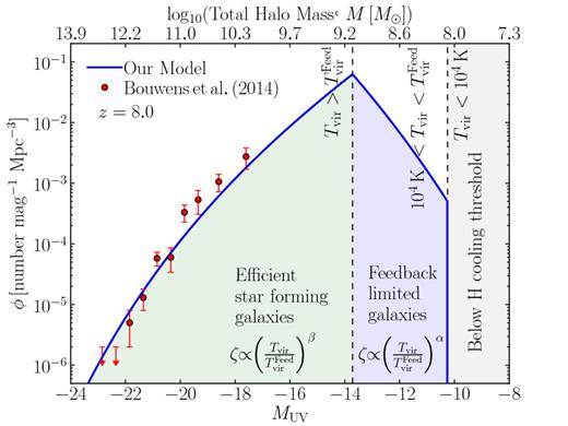
Here, we allow for a critical temperature threshold, |$T^{\rm Feed}_{\rm vir}$|, which can even be larger than 104 K. Below |$T^{\rm Feed}_{\rm vir}$| (but above 104 K), haloes are still sufficiently large to produce low-mass galaxies; however, their potential wells are not deep enough to retain supernovae-driven outflows that quench star formation and their corresponding contribution to reionization (e.g. Springel & Hernquist 2003). In this work, we allow |$T^{\rm Feed}_{\rm vir}$| to vary within the range |$T^{\rm Feed}_{\rm vir}\in [10^{4},2\times 10^{5}]$| K, with the lower limit set by the atomic cooling threshold and the upper limit consistent with observed high-z Lyman break galaxies (see for example Fig. 1).
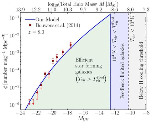
A schematic picture of the z = 8 non-ionizing UV luminosity function (blue curve) from our fiducial single population reionization model (used for the mock observation) characterized by a threshold temperature of |$T^{\rm Feed}_{\rm vir} = 3\times 10^{4}\,{\rm K}$| (M ∼ 108.78 M⊙ at z = 8). Haloes above |$T^{\rm Feed}_{\rm vir}$| host typical star-forming galaxies contributing to the reionization of the IGM (green shaded region). Below |$T^{\rm Feed}_{\rm vir}$|, haloes are small enough to be affected by internal feedback processes (blue shaded region). At Tvir < 104 K (M ∼ 108.06 M⊙ at z = 8), gas can no longer efficiently cool to accrete on to haloes. Note that the model curve at |$T_{\rm vir} > T^{\rm Feed}_{\rm vir}$| is obtained from a power-law fit to the halo mass as a function of UV magnitude recovered from abundance matching, which we can use to imply that for our fiducial choice of a constant ionizing efficiency we roughly obtain the scaling, fesc ∝ M0.32 (see the text for further discussions).
Likelihood Statistics
Although |$21$|CMFAST produces 3D maps of the 21 cm brightness temperature, we require a goodness of fit statistic in order to quantitatively compare an EoR realization with the mock observation. We choose the common spherically averaged 21 cm PS, |$\Delta ^{2}_{21}(k,z) \equiv k^{3}/(2\pi ^{2}V)\,\delta \bar{T}^{2}_{\rm b}(z)\,\langle |\delta _{21}(\boldsymbol {k},z)|^{2}\rangle _{k}$| where |$\delta _{21}(\boldsymbol {x},z) \equiv \delta T_{\rm b}(\boldsymbol {x},z)/\delta \bar{T}_{\rm b}(z) -1$|, to be this statistic. It is important to note that while we restrict our default analysis to |$\Delta ^{2}_{21}(k,z)$|, in principle any statistical measure of the cosmic 21 cm signal could be used in our framework.
The MCMC driver
An MCMC based EoR tool is a computationally challenging prospect since each step in the computation chain requires a |$21$|CMFAST realization. For reference, computing a 1283 21 cm realization at a single redshift takes ∼3 s using a single core. This is efficient, however, it is a case of diminishing returns if we attempt to improve the computation time using the inbuilt multithreading of |$21$|CMFAST. Therefore, constructing an MCMC analysis tool which samples |$21$|CMFAST utilizing existing serial MCMC algorithms such as Metropolis–Hastings (Metropolis et al. 1953; Hastings 1970), which require multiple long computation chains, would be too computationally inefficient.
In recent years, several new, more efficient and parallel MCMC algorithms have been developed. Once such algorithm is the affine invariant ensemble sampler developed by Goodman & Weare (2010). This algorithm has since been modified and improved before being released as the publicly available python module emcee by Foreman-Mackey et al. (2013). Recently, Akeret et al. (2013) discussed the virtues of adopting these computational algorithms for applications of cosmological parameter sampling. These authors released an easy to implement, massively parallel, publicly available python module cosmohammer which has already been extensibly adopted for a wide variety of cosmological application. We therefore choose to build |$21$|CMMC using a modified version of cosmohammer which performs our MCMC reionization parameter sampling by calling |$21$|CMFAST at each step in the computation chain to compute the log-likelihood.
Telescope noise profiles
To illustrate the performance of |$21$|CMMC for current and future 21 cm experiments, we compute the telescope sensitivities using the python module |$21$|cmsense8 (Pober et al. 2013, 2014). In this section, we outline only the specifics and assumptions we make in producing our realistic telescope noise profiles, summarizing the key telescope parameters in Table 1, and defer the reader to the more detailed discussions within Parsons et al. (2012a) and Pober et al. (2013, 2014).
Summary of telescope parameters we use to compute sensitivity profiles (see the text for further details).
| Parameter | LOFAR | HERA | SKA |
|---|---|---|---|
| Telescope antennas | 48 | 331 | 866 |
| Diameter (m) | 30.8 | 14 | 35 |
| Collecting area (m2) | 35 762 | 50 953 | 833 190 |
| Trec (K) | 140 | 100 | 0.1Tsky + 40 |
| Bandwidth (MHz) | 8 | 8 | 8 |
| Integration time (hrs) | 1000 | 1000 | 1000 |
| Parameter | LOFAR | HERA | SKA |
|---|---|---|---|
| Telescope antennas | 48 | 331 | 866 |
| Diameter (m) | 30.8 | 14 | 35 |
| Collecting area (m2) | 35 762 | 50 953 | 833 190 |
| Trec (K) | 140 | 100 | 0.1Tsky + 40 |
| Bandwidth (MHz) | 8 | 8 | 8 |
| Integration time (hrs) | 1000 | 1000 | 1000 |
Of great concern for 21 cm experiments is the estimation and removal of the bright foreground emission. Most notable of these are the chromatic effects due to how the interferometric array's uv coverage depends on frequency. It has been shown that these effects do not lead to mode-mixing across all frequencies, but instead localize the majority of the foreground noise into a foreground ‘wedge’ within cylindrical 2D k-space (Datta, Bowman & Carilli 2010; Morales et al. 2012; Parsons et al. 2012b; Trott, Wayth & Tingay 2012; Vedantham, Shankar & Subrahmanyan 2012; Thyagarajan et al. 2013; Liu, Parsons & Trott 2014a,b). This results in a relatively pristine observing window where the cosmological 21 cm signal is dominated only by thermal noise. However, it is still uncertain where to define the transition from the foreground ‘wedge’ to the EoR observing window.
Moreover, the summation over redundant baselines within an array configuration can reduce uncertainties in the thermal noise estimates (Parsons et al. 2012a). However, the gain depends on whether they are perfectly or partially coherent (Hazelton, Morales & Sullivan 2013).
In Pober et al. (2014), these authors consider numerous foreground removal strategies, including a variety of treatments for the summation over redundant baselines and how to define the transition from the foreground ‘wedge’. We defer the reader to their work for more detailed discussions, and highlight that throughout this work, we adopt what they refer to as their ‘moderate’ foreground removal. For this, we assume a fixed location of the foreground ‘wedge’ to extend Δk∥ = 0.1 h Mpc−1 beyond the horizon limit (Pober et al. 2014) and compute our estimates of the thermal noise PS sampling only k-modes that fall within the EoR observing window. This strategy further assumes the coherent addition of all redundant baselines.
We include another level of conservatism to our errors, applying a strict k-mode cut to our 21 cm PS. We sample only modes above |k| = 0.15 Mpc−1. Following the moderate foreground removal strategy of Pober et al. (2014), it effectively turns out that there is limited information available below this k-mode; however, we still apply this strict cut on top of the estimated total noise PS. Modes with |k| ≥ 0.15 Mpc−1 can still be affected by the foreground ‘wedge’ due to its spherically asymmetric structure, hence we apply both cuts.
Within this work, we restrict our analysis to three telescope designs (LOFAR, HERA and the SKA). In Pober et al. (2014), these authors qualitatively compare the merits of a variety of telescope designs through a measurement of the overall sensitivity of the 21 cm PS. To perform this direct comparison, these authors set a variety of design specific parameters to be equivalent. Instead, we perform our comparison using the exact design specifics of each experiment as outlined below. Note, the difference is marginal, however using system specific parameters we better mimic the expected overall sensitivities of the modelled telescope. For all, we model Tsky using the frequency dependent scaling |$T_{\rm sky} = 60\left(\frac{\nu }{300\, {\rm MHz}}\right)^{-2.55} {\rm K}$| (Thompson, Moran & Swenson 2007).
LOFAR: we model LOFAR using the antennas positions listed in van Haarlem et al. (2013). Following the approach of Pober et al. (2014), we focus solely on the Netherlands core for the purposes of detecting the 21 cm PS assuming that all 48 high-band antennas (HBA) stations can be correlated separately maximizing the total number of redundant baselines. We assume Trec = 140 K consistent with Jensen et al. (2013).
HERA: we follow the design specifics outlined in Beardsley et al. (2015), where they propose a final design including 331 antennas. Each antennas is 14 m in diameter closely packed into a hexagonal configuration to maximize the total number of redundant baselines (Parsons et al. 2012a). While the total observing area for HERA is an order of magnitude lower than the SKA, its design is optimized specifically for PS measurements allowing for comparable sensitivity (Pober et al. 2014).9 However, our 331 antennas telescope is smaller than the larger 547 antennas instrument proposed by these authors, therefore, our design performs more as an intermediate instrument. For HERA, we model the total system temperature as Tsys = 100 + TskyK.
SKA: we mimic the current design brief for the SKA-low Phase 1 instrument outlined in the SKA System Baseline Design document.10 Specifically, SKA-low Phase 1 includes a total of 911 35 m antennas stations, with 866 stations normally distributed in radius within a core extending out to a radius of ∼2 km and a further 45 stations arranged into three spiral arms each with 15 stations extending to ∼50 km. For our SKA design, we include only the core stations, as the spiral arms add little to the PS sensitivity. As in Pober et al. (2014), we model the central core of SKA as a hexagon to maximize baseline redundancy, however our core extends out to a radius of ∼300 m which includes a total of 218 telescope antennas. We then randomly place the telescope antennas normalizing to ensure we contain 433 and 650 telescopes within a radii of 600 and 1000 m and randomly place the remaining 216 antennas at a radii larger than 1000 m. The total SKA system temperature is modelled as outlined in the SKA System Baseline Design, Tsys = 1.1Tsky + 40K.
The |$21$|CMFAST pipeline
Eventually |$21$|CMMC will be performed on actual observations. However for this proof of concept, we first create mock observations of the cosmic EoR signal and generate sensitivities for various instruments.11 Using |$21$|CMFAST, we perform a high-resolution, large-box realization of our fiducial EoR model, simulated within a 5003 cMpc3 box with an initial grid of 15363 voxels smoothed on to a 2563 grid. We then calculate the 21 cm PS from this simulation at several different redshifts and compute the total noise contribution from thermal and sample variance using |$21$|cmsense. In addition to the thermal noise and sample variance, we add an additional uncertainty due to EoR modelling, accounting for, e.g. differences in the implementation of RT (e.g. Iliev et al. 2006) and errors in seminumerical approximations (e.g. Zahn et al. 2011). In other words, even if we have a well behaved Universe characterized exactly by our 3 or 5 parameter models, the simulated PS will be different from the true one due to the numerical implementation. We assume for this a constant multiplicative error of 25 per cent, guided by the observed 10–30 per cent difference at the relevant scales between |$21$|CMFAST and the cosmological RT simulations in Zahn et al. (2011). For each mock observation of the 21 cm PS, we add this 25 per cent error in quadrature with the noise contribution from equation (6). In principle this would be a correlated error, however, at this stage a constant multiplicative factor is sufficient. Below, we include some results excluding this error, showing the maximum information which can be extracted from the signal assuming a perfect characterization of modelling uncertainties.
To sample the reionization parameter space in |$21$|CMMC, we perform a smaller, lower resolution EoR simulation. Using a different set of initial conditions to the mock observations, we simulate a 2503 cMpc3 volume with an initial grid of 7683 voxels smoothed down on to a 1283 grid. Our two simulations are both sampled at the same physical resolution (∼2 Mpc), and resampled by the same factor of 6 from the initial density grid to ensure convergence between the recovered 21 cm PS from the mock observation and the PS from the smaller 1283 simulations. To account for the impact of shot noise on the smallest spatial modes (largest k) within these low-resolution simulations, we apply an additional cut at k ≥ 1.0 Mpc−1.
At each step in the MCMC algorithm, we compute the 21 cm PS corresponding to that point in our astrophysical parameter space using the 3D realization from |$21$|CMFAST. We compute its likelihood using the χ2 statistic between k = 0.15 and 1.0 Mpc−1 to assess whether to accept or reject the new proposed set of EoR parameters.
Finally, we briefly discuss the improvements in our method to sample the astrophysical EoR parameter space, relative to previous works. These previous approaches have been restricted to either sampling a fixed, course grid of reionization models (e.g. Barkana 2009; Mesinger et al. 2012; Zahn et al. 2012) or the fundamental assumption of Gaussian errors in Fisher Matrix applications (Pober et al. 2014; although new methods exist to overcome this assumption, e.g. Joachimi & Taylor 2011; Sellentin, Quartin & Amendola 2014). Instead, with a Bayesian MCMC framework, we are able to more efficiently sample the EoR parameter space and by construction obtain direct estimates of the individual probability distribution functions (PDFs) of the EoR parameters, removing the a priori assumptions on the intrinsic probability distribution (i.e. Gaussian). Moreover, by sampling over 105 realizations within |$21$|CMMC this allows us to sample many features within the EoR parameter space not visible in course-grid models. Additionally, this allows for the better characterization of parameter degeneracies, which is a problem for Fisher Matrix analyses.
SINGLE IONIZING GALAXY POPULATION
Building physical intuition
UV luminosity function
It is first constructive to illustrate how this EoR model would appear with respect to current observations. In Fig. 1, we provide a schematic picture of our single ionizing galaxy population compared to the observed non-ionizing (∼ 1500 Å) UV luminosity function at z = 8 of Bouwens et al. (2014). To obtain the UV luminosity of our galaxy population, we use the Schechter function parameter values described in Kuhlen & Faucher-Giguère (2012) and abundance matching to estimate the host halo mass as a function of the UV magnitude, M(MUV). Fitting this expression as a power law, we convert our |$T^{\rm Feed}_{\rm vir}$| into a UV magnitude which produces a sharp drop in the UV luminosity function at MUV = −12.6 (M ∼ 108.78 M⊙). By construction, the non-ionizing UV luminosity function matches the observational data and we extrapolate down into the faint-end until |$T^{\rm Feed}_{\rm vir}$|, below which no ionizing photons are produced/escape the galaxy. In our illustrative model, this drop, tracing fundamental galaxy formation physics, is well beyond the sensitivity limits even for JWST (e.g. Salvaterra, Ferrara & Dayal 2011), showcasing the power of our approach.
The UV luminosity function with an appropriate dust model can constrain the star formation rate, which (approximately) collapses the uncertainty in the ionizing emissivity to just that in the escape fraction, fesc. In other words, the total ionizing luminosity, Lion is roughly proportional to the product of the non-ionzing UV luminosity (LUV) and fesc: Lion(M) ∝ fesc(M)LUV(M). Our fiducial choice of a constant ζ implies Lion ∝ M, from which we can obtain an expression for LUV(M) using our power-law expression for M(MUV) to recover LUV(M) ∝ M0.68 for the faint end of the luminosity function. Therefore, our illustrative, single population model at z = 8 roughly translates to fesc ∝ M0.32.
How does the 21 cm PS depend on the EoR parameters?
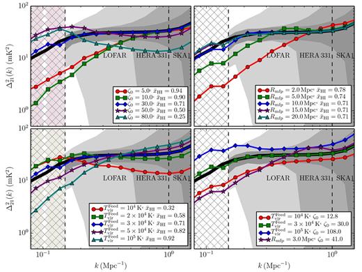
The 21 cm PS at z = 9 for various values of our three reionization parameters, ζ0, Rmfp and |$T^{\rm Feed}_{\rm vir}$|. In all panels, the thick black curve corresponds to our fiducial reionization model, with (ζ0, Rmfp, |$T^{\rm Feed}_{\rm vir}$|) = (30, 15 Mpc, 3 × 10⁴ K) and a neutral fraction of |$\bar{x}_{\mathrm{H\,{\small I}}{}} = 0.71$|. Light to dark shaded regions correspond to the 1σ errors of the total noise PS (see Sections 2.4 and 2.5) for the three 21 cm experiments we consider in this analysis (LOFAR, HERA and SKA), including a 25 per cent modelling uncertainty. Dashed vertical lines at k = 0.15 and k = 1.0 Mpc−1 demarcate the physical scales on which we choose to fit the 21 cm PS, while the hatched region corresponds to the foreground dominated region. We show the impact of the ionizing efficiency ζ0 (top left), the maximum horizon for ionizing photons, Rmfp (top right) and the minimum virial temperature of star-forming galaxies, |$T^{\rm Feed}_{\rm vir}$| (bottom left). Bottom right: the 21 cm PS corresponding to different EoR parameters, but at the same EoR epoch (|$\bar{x}_{\mathrm{H\,{\small I}}{}}$|) as the fiducial simulation.
Before reionization gets well underway (|$\bar{x}_{\mathrm{H\,{\small I}}{}} > 0.9$|) |$\Delta ^{2}_{21}$| closely follows the matter density PS, |$\Delta ^{2}_{\delta \delta }$|. Initially, cosmic H ii bubbles grow around biased density peaks hosting galaxies. This causes the large-scale power to drop due to the increased (negative) contribution from the cross-correlation term, |$\Delta ^{2}_{\delta {\rm x}}$|. As time evolves (|$\bar{x}_{\mathrm{H\,{\small I}}{}}$| decreases), the H ii bubbles become more numerous (with the increasing population of ionizing sources) and begin to overlap, increasing the contribution from the ionization PS, |$\Delta ^{2}_{\rm xx}$|. Eventually, this term begins to dominate, resulting in an overall increase in the total power in |$\Delta ^{2}_{21}$| across all scales. At |$\bar{x}_{\mathrm{H\,{\small I}}{}} = 0.5$|, the large-scale power peaks. As the H ii bubbles grow and overlap, the peak power in |$\Delta ^{2}_{21}$| shifts to larger physical scales (smaller k) as |$\Delta ^{2}_{\rm xx}$| is sensitive to the physical size of the H ii regions. At the same time, the power on small scales begins to drop as the number of small, isolated H ii regions decreases.
This generic PS evolution during the EoR is evident in the first three panels of Fig. 2 (see also, e.g. McQuinn et al. 2007; Lidz et al. 2008; Friedrich et al. 2011). A larger value of ζ0 corresponds to a more advanced EoR at z = 9, as galaxies are more efficient at producing ionizing photons. Similarly, a smaller value of |$T^{\rm Feed}_{\rm vir}$| results in a more advanced EoR, as smaller, more abundant galaxies can efficiently form stars. The progress of the EoR is less sensitive to variation in Rmfp (second panel); instead this maximum horizon for the ionizing photons produces a prominent ‘knee’ in the PS, suppressing coherent ionization structure on large scales (e.g. Alvarez & Abel 2012; Mesinger et al. 2012).
The PS is not however entirely determined by |$\bar{x}_{\mathrm{H\,{\small I}}{}}$|. In the final panel of Fig. 2, we illustrate the impact of our EoR parameters at a fixed IGM neutral fraction of |$\bar{x}_{\mathrm{H\,{\small I}}{}} = 0.71$| (i.e. all at the equivalent stage of reionization). For example, if the EoR is driven by more biased, larger mass haloes (larger |$T^{\rm Feed}_{\rm vir}$|), their relative dearth must be compensated for by a higher ionizing efficiency. This results in an EoR morphology with larger, more isolated cosmic H ii patches (e.g. McQuinn et al. 2007). |$\Delta ^{2}_{\rm xx}$| is more peaked on large scales, with a decrease in |$\Delta ^{2}_{\delta {\rm x}}$|. As a result, the 21 cm PS is higher, with a more prominent large-scale ‘bump’ tracing the typical H ii region size. Also explicitly evident in the last panel is the prominent ‘knee’ feature, imprinted by small values of Rmfp. Here, for Rmfp = 3 Mpc (blue curve), the ionization PS peaks on much smaller scales, with a sharp drop in large-scale power compared to the other curves computed with Rmfp = 15 Mpc. Therefore, the 21 cm PS contains information on both the EoR epoch (i.e. |$\bar{x}_{\mathrm{H\,{\small I}}{}}$|), as well as independent (i.e. at fixed |$\bar{x}_{\mathrm{H\,{\small I}}{}}$|) information on the properties of galaxies and the IGM.
In all panels, we provide the estimated 1σ errors on the 21 cm PS for each of the considered 21 cm experiments, including the additional 25 per cent modelling uncertainty. It is immediately obvious that LOFAR will have difficulty discriminating among various models, having to rely on the largest scales close to the foreground-dominated regime. HERA and the SKA on the other hand should be able to recover meaningful constraints on EoR parameters, with the large-scales limited by the additional 25 per cent modelling uncertainty we include. On smaller spatial scales, SKA performs considerably better than HERA.
Single epoch observation of the 21 cm PS
21 cm experiments have coverage over a large bandwidth (e.g. 50–350 MHz for the SKA allowing for observations to z ≲ 28). However, foregrounds and high data rates can limit the coverage to narrower instantaneous bandwidths. Hence, we begin by analysing an observation at a single redshift (assuming our fiducial bandwidth of 8 MHz), before moving on to a broader bandpass observation. We restrict our analysis to only second-generation 21 cm experiments, HERA and the SKA, since with a single bandwidth the first-generation instruments will only achieve a marginal detection at best (e.g. Mesinger et al. 2014; Pober et al. 2014; see also Fig. 2).
In Fig. 3, we compare the outputs of |$21$|CMMC for both HERA (red curve) and SKA (blue curve) for an assumed single z = 9 observation of our fiducial 21 cm PS with a total integration time of 1000 h. In this figure, and for the remainder of this work we assume uniform priors on all recovered parameters within their allowed ranges outlined in Section 2.1. The dashed vertical lines denote the mock observation values. Across the diagonal panels of this figure we provide the 1D marginalized PDFs for each of our EoR parameters. In the top-right panel, we provide the marginalized 1D PDFs of the IGM neutral fraction. Additionally, we choose to renormalize all 1D PDFs to have the peak probability equal to unity to better visually emphasize the shape and width of the recovered distribution. In the lower-left corner of Fig. 3, we show the 2D joint marginalized likelihood distributions. In each panel, the cross denotes the location of our fiducial EoR parameters. For each, we construct both the 1σ and 2σ contours (thick and thin lines, respectively), by computing a smoothed 2D histogram of the entire MCMC sample and estimating the likelihood contours which enclose 68 and 95 per cent of the data sample, respectively.
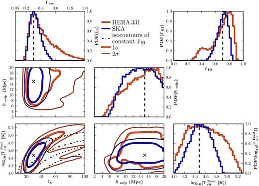
The recovered constraints from |$21$|CMMC on our three parameter EoR model parameters for a single (z = 9) 1000 h observation of the 21 cm PS obtained with HERA (red curve) and the SKA (blue curve). In the diagonal panels, we provide the 1D marginalized PDFs for each of our EoR model parameters (ζ0, Rmfp and log10|$(T^{\rm Feed}_{\rm vir}),$| respectively) and we highlight our fiducial choice for each by the vertical dashed line. Additionally, we cast our ionizing efficiency, ζ0, into a corresponding escape fraction, fesc, on the top axis (simply using the fiducial values in equation 2). In the upper-right panel, we provide the 1D PDF of the recovered IGM neutral fraction where the vertical dashed line corresponds to the neutral fraction of the mock 21 cm PS observation (|$\bar{x}_{\mathrm{H\,{\small I}}{}} = 0.71$|). Finally, in the lower-left corner we provide the 1 (thick) and 2σ (thin) 2D joint marginalized likelihood contours for our three EoR parameters (crosses denote their fiducial values, and the dot–dashed curves correspond to isocontours for |$\bar{x}_{\mathrm{H\,{\small I}}{}}$| of 20, 40, 60 and 80 per cent from bottom to top).
For all EoR parameters, the recovered PDFs are centred around their input fiducial parameters, highlighting the strong performance of |$21$|CMMC at recovering our input model. This is despite the asymmetric distributions of the recovered PDFs, emphasizing the strength of the MCMC approach within |$21$|CMMC. Comparing these two 21 cm experiments, we note the significant improvement achievable with the increased sensitivity of the SKA. This can easily be seen in the case of both ζ0 and |$T^{\rm Feed}_{\rm vir}$|, where the widths of the 1D PDFs, as well as the 2D joint likelihood contours, are noticeably tighter for SKA than for HERA.
The improved constraints from the SKA relative to HERA can be best explained by referring to Fig. 2. We observe that while the sensitivity at large scales for both SKA and HERA are comparable, only the SKA is capable of probing the available small-scale information. Given the degenerate nature of the EoR parameters, by accessing this additional shape information tighter constraints are achievable. While it is not sufficient to break the degeneracies it does reduce their amplitude, substantially limiting the allowed EoR parameter space. It is important to note that with only a single redshift observation, the uncertainty is large and the likelihood is non-Gaussian distributed. Nevertheless, our Bayesian MCMC framework captures parameter constraints and degeneracies, recovering the actual shape of the likelihood distribution (without the Gaussian assumptions of the Fisher matrix formalism; Pober et al. 2014).
In the ζ0-|${\rm log}_{10}T^{\rm Feed}_{\rm vir}$| plane for HERA in lower-left panel of Fig. 3, we observe at the 95 per cent confidence level a multimodal distribution for ζ0 and |$T^{\rm Feed}_{\rm vir}$| as highlighted by the lower streaks for high ζ0 and low |$T^{\rm Feed}_{\rm vir}$|. This region of parameter space is capable of reionizing the IGM earlier than our fiducial EoR model, due to a brighter population of lower mass galaxies (see Section 3.1.2). This is highlighted by overlaying the |$\bar{x}_{\mathrm{H\,{\small I}}{}}$| isocontours for the EoR parameter space, where it is clear that these two streaks reproduce different IGM neutral fractions. Correspondingly, these models result in a smaller, secondary feature around |$\bar{x}_{\mathrm{H\,{\small I}}{}} = 0.4$| in the IGM neutral fraction PDF. Models in this region of the EoR parameter space have similar large-scale 21 cm power, but different small-scale structure which HERA cannot differentiate. The SKA, due to its higher sensitivity on small scales does not exhibit the same behaviour. Alternatively, these degeneracies can be broken with additional redshift observations which constrain the redshift evolution of the large-scale power (see below).
In order to quantitatively assess the performance of |$21$|CMMC, we choose to report the median value of each EoR parameter and the associated 16th and 84th percentiles. This choice follows on from the fact that the recovered 1D PDFs do not need to be normally distributed within the Bayesian MCMC framework, as observed in the case of HERA in Fig. 3. In Table 2, we summarize the recovered EoR parameter constraints for each of the 21 cm experiments from a single epoch observation of the 21 cm PS.
The median recovered values (and associated 16th and 84th percentile errors) for our three EoR model parameters, ζ0, Rmfp and |$T^{\rm Feed}_{\rm vir}$| and the associated IGM neutral fraction, |$\bar{x}_{\mathrm{H\,{\small I}}{}}$|. We assume a total 1000 h integration time for a single epoch (z = 9) observation of the 21 cm PS and compare the recovered constraints for HERA, with and without a z = 7 IGM neutral fraction prior (|$\bar{x}_{\mathrm{H\,{\small I}}{}} > 0.05$|), and for the SKA, respectively. Our fiducial parameter set is (ζ0, Rmfp, |${\rm log}_{10}T^{\rm Feed}_{\rm vir}$|) = (30, 15 Mpc, 4.48) which results in an IGM neutral fraction of |$\bar{x}_{\mathrm{H\,{\small I}}{}} = 0.71$|.
| Instrument | Parameter | |$\bar{x}_{\mathrm{H\,{\small I}}{}}$| | ||
|---|---|---|---|---|
| (single-z) | ζ0 | Rmfp | log10|$(T^{\rm Feed}_{\rm vir})$| | z = 9 |
| HERA 331 | $38.38{{\scriptstyle {\begin{array}{c}
+22.43 \\
-11.33\end{array}}}}$ | $14.34{{\scriptstyle {\begin{array}{c}
+3.72 \\
-4.95\end{array}}}}$ | $4.57{{\scriptstyle {\begin{array}
{c}+0.36 \\
-0.32\end{array}}}}$ | $0.73{{\scriptstyle {\begin{array}{c}
+0.10 \\
-0.21\end{array}}}}$ |
| HERA 331 (with prior) | $38.37{{\scriptstyle {\begin{array}{c}
+20.86 \\
-11.53\end{array}}}}$ | $13.88{{\scriptstyle {\begin{array}{c}
+3.76 \\
-4.39\end{array}}}}$ | $4.65{{\scriptstyle {\begin{array}{c}
+0.32 \\
-0.35\end{array}}}}$ | $0.75{{\scriptstyle {\begin{array}{c}
+0.09 \\
-0.13\end{array}}}}$ |
| SKA | $32.11{{\scriptstyle {\begin{array}{c}
+8.32 \\
-6.47\end{array}}}}$ | $13.78{{\scriptstyle {\begin{array}{c}
+3.87 \\
-4.09\end{array}}}}$ | $4.50{{\scriptstyle {\begin{array}{c}
+0.20 \\
-0.21\end{array}}}}$ | $0.71{{\scriptstyle {\begin{array}{c}
+0.07 \\
-0.09\end{array}}}}$ |
For HERA, we note that while both Rmfp and |$T^{\rm Feed}_{\rm vir}$| (also |$\bar{x}_{\mathrm{H\,{\small I}}{}}$|), are recovered to within 5 per cent of our fiducial parameters, in the case of ζ0 we over predict the expected value by close to 30 per cent. This is not surprising given the mild positive asymmetry observed in the recovered 1D PDF for ζ0. Since we choose to report the median recovered value for all EoR parameters, whenever we recover an asymmetric distribution our reported value can be shifted away from the input fiducial value. Despite the skewness, the 16th and 84th percentiles should for the most part enclose our fiducial values.
In the case of the SKA, we are able to recover all EoR parameters values at less than 10 per cent deviation from their fiducial values. While the errors on Rmfp remain relatively consistent with those for HERA, we observe a reduction of close to a factor of 2 (3) for the lower (upper) 1σ bounds on ζ0 and a 30 per cent reduction on the 1σ errors on |$T^{\rm Feed}_{\rm vir}$|. We note a reduction also of approximately 25 per cent on the recovered 1σ errors for the IGM neutral fraction.
Single redshift observation with a neutral fraction prior
In the previous section, we noted that the same large-scale power could occur at different IGM neutral fractions. This degeneracy can be broken with increased small-scale sensitivity (as in the case of SKA). Here, we investigate whether we can improve upon the available constraining power from a single redshift observation by instead including a prior on the IGM neutral fraction from observations at the tail end of the reionization epoch. For example, such constraints can be obtained from the spectra of high-z quasars such as ULAS J1120+0641 (Bolton et al. 2011; Mortlock et al. 2011) or from the observed drop in Lyman-α emission from high-z galaxies (e.g. Caruana et al. 2014; Dijkstra et al. 2014; Pentericci et al. 2014; Mesinger et al. 2015). Here, we consider a purely illustrative conservative lower limit on the IGM neutral fraction at z = 7 of 5 per cent. We caution however that priors on different epochs can make our results more model dependent. For example, our fiducial EoR model does not allow for a redshift evolution in the reionization parameters. This is straightforward to account for, however, we postpone it to future work.
In Fig. 4, we compare the recovered EoR parameter constraints for HERA from the same 1000 h observation of the 21 cm PS at z = 9, following the inclusion of the IGM neutral fraction prior at z = 7. Additionally, in Table 2, we again provide the recovered median and 1σ errors for our EoR parameters. After the inclusion of the z = 7 neutral fraction prior we observe only a very marginal improvement in either the median recovered values or their 1σ errors and this is equivalently shown by the slightly narrower widths of the recovered 1D PDFs.
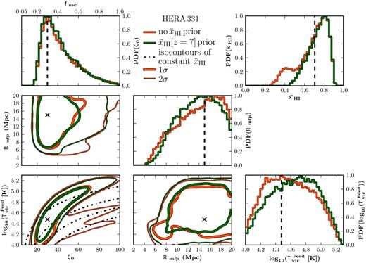
Similar to Fig. 3, except now we compare the impact of including an IGM neutral fraction prior for a single (z = 9) 1000 h observation with HERA. We consider an IGM neutral fraction prior at z = 7 of |$\bar{x}_{\mathrm{H\,{\small I}}{}} > 0.05$| (a conservative choice motivated by recent QSO and LAE observations; green curves) and without a neutral fraction prior (red curve). The inclusion of a neutral fraction prior improves the constraints on the reionization parameters from a single z observation.
However, in the case of the 2D joint likelihood distributions we are able to observe an improvement in the allowed EoR parameter space. Specifically, focusing again on the ζ0-|${\rm log}_{10}T^{\rm Feed}_{\rm vir}$| plane, while the 1σ errors are only marginally improved, the 2σ contours are notably reduced. Most importantly, the IGM neutral fraction prior removes the second degenerate streak which marginally allowed a significantly different reionization history in the absence of the prior when observed with HERA. This can clearly be seen from the removal of the previously noted secondary bump at |$\bar{x}_{\mathrm{H\,{\small I}}{}} = 0.4$| in the IGM neutral fraction PDF. By imposing that the IGM must at least be 5 per cent neutral at z = 7, this rules out reionization scenarios which would otherwise predict an early end to the reionization epoch from a single redshift observation of the 21 cm PS. This highlights the importance of the additional leverage gained from probing the reionization history at improving the EoR reionization constraints, especially in the absence of strong telescope sensitivity at small scales.
The level of improvement achievable from an IGM neutral fraction prior on a single epoch measurement of the 21 cm PS depends on numerous factors. First, imposing a harder prior than our conservative choice would allow increased constraining power on the allowed EoR parameter space. Secondly, with decreasing telescope sensitivity, a neutral fraction prior becomes more important, as knowledge of the EoR history compensates for poor single epoch PS coverage. It is feasible that with improved foreground removal strategies, a marginal detection of the 21 cm PS could be achieved with first-generation instruments (Pober et al. 2014). Therefore, in this scenario, a neutral fraction prior would be of vital importance for improving the available EoR constraining power.
Finally, due to the flexibility of |$21$|CMMC we emphasize that it is straightforward to additionally include direct priors on our model EoR parameters motivated by current and upcoming observations and theoretical advances. Given the observed degeneracies between the EoR parameters within this model, it is clear that including priors on our model parameters would notably improve the overall constraining power.
Combining multiple redshift observations
Here, we consider combining multiple epoch observations of the 21 cm PS, assuming a broader instantaneous bandwidth is available for the EoR observations. However, this comes at the cost of increased model dependence. For example, our three empirical EoR parameters are redshift-independent, whereas physically, we would expect each parameter to vary with redshift across the reionization epoch. In this sense, our astrophysical parameters can be thought of as ‘effective’ EoR properties, averaging over any redshift evolution. In future, we will explicitly include a generalized redshift evolution for EoR parameters (e.g. Barkana 2009; Mesinger et al. 2012; Zahn et al. 2012).
To combine all the available information across the multiple epochs and differentiate between the sampled EoR parameters, we compute the total maximum likelihood fit of the EoR model, obtained by linearly combining the individual χ2 statistics from each redshift. In principle, we could instead perform a weighted summation to estimate the total maximum likelihood; however, in neglecting to do so our errors are more conservative.
In Fig. 5, we compare the recovered 1D marginalized PDFs and 2D marginalized likelihood contours for our three fiducial EoR parameters (ζ0, Rmfp and log10|$(T^{\rm Feed}_{\rm vir})$|). For this, we assume three independent 1000 h observations of the 21 cm PS at z = 8, 9 and 10 for LOFAR (turquoise), HERA (red) and SKA (blue) each with a 1000 h integration time. In Fig. 6, we provide the recovered 1D PDFs of the IGM neutral fraction from each individual epoch. Note, for our fiducial EoR model, the corresponding IGM neutral fractions are |$\bar{x}_{\mathrm{H\,{\small I}}{}}$| = 0.48, 0.71 and 0.83, respectively. Finally, in Table 3 we provide the recovered median, 16th and 84th percentiles for each EoR parameter and the corresponding IGM neutral fraction.
![The recovered constraints from $21$CMMC on our reionization model parameters from combining three independent (z = 8, 9 and 10) 1000 h observations of the 21 cm PS. We compare the different telescope arrays, LOFAR (turquoise), HERA (red) and SKA (blue). Across the diagonal panels, we provide the 1D marginalized PDFs for each of our reionization parameters [ζ0, Rmfp and log10$(T^{\rm Feed}_{\rm vir}),$ respectively] and highlight our fiducial model parameter by a vertical dashed line. Additionally, we provide the 1 (thick) and 2σ (thin) 2D joint marginalized likelihood contours for our three reionization parameters in the lower-left corner of the figure (crosses mark our fiducial reionization parameters). Including redshift information can significantly improve the constraints on each reionization parameter, and could even yield sufficient information to allow LOFAR to provide marginal constraints.](https://oup.silverchair-cdn.com/oup/backfile/Content_public/Journal/mnras/449/4/10.1093_mnras_stv571/1/m_stv571fig5.jpeg?Expires=1716422221&Signature=wRD4J8u8YHJmRWNLbp6MRwlFZ4YtYl2jvnOtsN0ue4WwCgR8W0L9pJIkonsu9RCGWs5oCwh-nBXJmJwUNMPVKTlFeUJafIB5nDYIdBoJqIh9PIV3PNek0C3UQ~5T8C4o0jkObKENNU4M48qW-0BbjqQKZH-XcJgXLfyYTVApg4~rP5W5Hq4JOd5eMBzXMbJg-rk4IrnhMMtDYJluCxBX7H2mOJl7D0dc0Fe4X0xqNTZ5jSAqPeuNalcxFDi-0m1AtEH0rYTgl0xN2SvssHecRuI7D8~us5XWTZ-idjEols~eD0HRSejDKXoJWw9H4~vPV4xijRoK1sZ84OQaMLCDNw__&Key-Pair-Id=APKAIE5G5CRDK6RD3PGA)
The recovered constraints from |$21$|CMMC on our reionization model parameters from combining three independent (z = 8, 9 and 10) 1000 h observations of the 21 cm PS. We compare the different telescope arrays, LOFAR (turquoise), HERA (red) and SKA (blue). Across the diagonal panels, we provide the 1D marginalized PDFs for each of our reionization parameters [ζ0, Rmfp and log10|$(T^{\rm Feed}_{\rm vir}),$| respectively] and highlight our fiducial model parameter by a vertical dashed line. Additionally, we provide the 1 (thick) and 2σ (thin) 2D joint marginalized likelihood contours for our three reionization parameters in the lower-left corner of the figure (crosses mark our fiducial reionization parameters). Including redshift information can significantly improve the constraints on each reionization parameter, and could even yield sufficient information to allow LOFAR to provide marginal constraints.
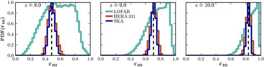
1D PDFs of the recovered IGM neutral fraction from our 1000 h observations of the 21 cm PS at z = 8 (left), z = 9 (centre) and z = 10 (right). Colours are the same as Fig. 5 and vertical dashed lines denote the neutral fraction of the mock 21 cm PS observations, |$\bar{x}_{\mathrm{H\,{\small I}}{}}$| = 0.48, 0.71 and 0.83, respectively.
Summary of the median recovered values (and associated 16th and 84th percentile errors) for our three EoR model parameters, ζ0, Rmfp and |$T^{\rm Feed}_{\rm vir}$| and the associated IGM neutral fraction, |$\bar{x}_{\mathrm{H\,{\small I}}{}}$|. We assume a total 1000 h integration time for each 21 cm PS observation at z = 8, 9 and 10 for LOFAR, HERA and the SKA, respectively. For both HERA and the SKA, we provide the recovered median values both including and excluding our 25 per cent modelling uncertainty (see Section 3.5). Our fiducial parameter set is (ζ0, Rmfp, |${\rm log}_{10}T^{\rm Feed}_{\rm vir}$|) = (30, 15 Mpc, 4.48) which results in an IGM neutral fraction of |$\bar{x}_{\mathrm{H\,{\small I}}{}} = 0.48$|, 0.71, 0.83 at z = 8, 9 and 10, respectively.
| Instrument | Parameter | |$\bar{x}_{\mathrm{H\,{\small I}}{}}$| | ||||
|---|---|---|---|---|---|---|
| (multi-z) | ζ0 | Rmfp (Mpc) | log10|$(T^{\rm Feed}_{\rm vir})$| | z = 8 | z = 9 | z = 10 |
| LOFAR | $45.21{{\scriptstyle {\begin{array}{c}
+26.27 \\
-18.06\end{array}}}}$ | $12.98{{\scriptstyle {\begin{array}{c}
+ 4.44\\
-5.50\end{array}}}}$ | $4.73{{\scriptstyle {\begin{array}{c}
+0.34 \\
-0.32\end{array}}}}$ | $0.57{{\scriptstyle {\begin{array}{c}
+ 0.20\\
-0.21\end{array}}}}$ | $0.76{{\scriptstyle {\begin{array}{c}
+0.13 \\
-0.15\end{array}}}}$ | $0.88{{\scriptstyle {\begin{array}{c}
+ 0.07\\
-0.10\end{array}}}}$ |
| HERA 331 | $30.17{{\scriptstyle {\begin{array}{c}
+7.60 \\
-5.35\end{array}}}}$ | $15.13{{\scriptstyle {\begin{array}{c}
+ 2.92\\
-3.01\end{array}}}}$ | $4.49{{\scriptstyle {\begin{array}{c}
+ 0.15\\
-0.16\end{array}}}}$ | $0.49{{\scriptstyle {\begin{array}{c}
+ 0.05\\
-0.05\end{array}}}}$ | $0.71{{\scriptstyle {\begin{array}{c}
+ 0.04\\
-0.04\end{array}}}}$ | $0.84{{\scriptstyle {\begin{array}{c}
+ 0.03\\
- 0.03\end{array}}}}$ |
| SKA | $30.04{{\scriptstyle {\begin{array}{c}
+ 5.65\\
-4.48\end{array}}}}$ | $15.22{{\scriptstyle {\begin{array}{c}
+ 2.82 \\
-2.91\end{array}}}}$ | $4.48{{\scriptstyle {\begin{array}{c}
+ 0.11\\
- 0.12\end{array}}}}$ | $0.49{{\scriptstyle {\begin{array}{c}
+0.04 \\
-0.04\end{array}}}}$ | $0.71{{\scriptstyle {\begin{array}{c}
+ 0.03\\
-0.03\end{array}}}}$ | $0.84{{\scriptstyle {\begin{array}{c}
+ 0.02\\
- 0.02\end{array}}}}$ |
| HERA 331 (w/o 25 per cent modelling uncertainty) | $28.78{{\scriptstyle {\begin{array}{c}
+ 2.54\\
-1.98\end{array}}}}$ | $14.33{{\scriptstyle {\begin{array}{c}
+ 1.12 \\
-0.93\end{array}}}}$ | $4.47{{\scriptstyle {\begin{array}{c}
+ 0.06\\
- 0.06\end{array}}}}$ | $0.47{{\scriptstyle {\begin{array}{c}
+0.02 \\
-0.02\end{array}}}}$ | $0.69{{\scriptstyle {\begin{array}{c}
+ 0.02\\
-0.02\end{array}}}}$ | $0.82{{\scriptstyle {\begin{array}{c}
+ 0.01\\
- 0.01\end{array}}}}$ |
| SKA (w/o 25 per cent modelling uncertainty) | $30.31{{\scriptstyle {\begin{array}{c}
+ 1.70\\
-1.62\end{array}}}}$ | $15.47{{\scriptstyle {\begin{array}{c}
+ 1.41 \\
-1.20\end{array}}}}$ | $4.48{{\scriptstyle {\begin{array}{c}
+ 0.04\\
- 0.04\end{array}}}}$ | $0.48{{\scriptstyle {\begin{array}{c}
+0.01 \\
-0.01\end{array}}}}$ | $0.71{{\scriptstyle {\begin{array}{c}
+ 0.01\\
-0.01\end{array}}}}$ | $0.83{{\scriptstyle {\begin{array}{c}
+ 0.01\\
- 0.01\end{array}}}}$ |
From Fig. 5, we observe the 1D PDFs and joint 2D likelihood contours to be almost indistinguishable between HERA and the SKA, with the SKA performing only marginally better. Furthermore, comparing with Fig. 3, the widths of both the 1D PDFs and 2D likelihood contours have significantly reduced, drastically in the case of HERA. This emphasises the strength of combining multiple epoch observations of the 21 cm PS (under the simple assumption they can be linearly combined). Quantitatively, we find little difference between the recovered constraints, with both instruments recovering median values of our EoR parameters to better than 1.5 per cent. Due to the improved constraining power from sampling the reionization history the recovered PDFs are now normally distributed. Therefore, we can estimate the total 1σ fractional error for each parameter. For SKA (HERA), we find errors of 16.7 (22.0) on ζ0, 17.8 (18.4) on Rmfp and 2.4 (3.3) per cent on log10|$(T^{\rm Feed}_{\rm vir})$|. Additionally, across all three observed epochs, both HERA and SKA tightly recover the expected IGM neutral fraction of our fiducial EoR model (see Fig. 6).
Importantly, while for a single epoch observation, the SKA notably outperforms HERA, the improvements available when probing the reionization history can make these two instruments comparable. By combining multiple epoch observations, these two experiments are able to pick up the same evolution in the 21 cm PS as the power rises and falls during reionization (see, e.g. Lidz et al. 2008 and our Section 3.1.2), compensating for their different sensitivity at small scales (for the case of these EoR models). Therefore, while the additional small-scale power can aid significantly in improving the constraining power from an individual observation, it only marginally improves the constraining power across multiple epochs.
For LOFAR, we find that by jointly combining multiple epoch observations we are now capable of recovering reionization constraints. As expected though, the quality of these constraints is drastically reduced compared to the second-generation experiments. Additionally, we recover broad marginalized 1D PDFs, which encompass the majority of the EoR parameter space and their asymmetric nature complicates a quantitative comparison with the second-generation experiments. We find LOFAR can only marginally rule out (at ∼2σ) either a rapid reionization (|$\bar{x}_{\mathrm{H\,{\small I}}{}} <0.2$| at z = 8) or a delayed/extended reionization (|$\bar{x}_{\mathrm{H\,{\small I}}{}} > 0.9$| at z = 8). However, this is still encouraging for the first generation of 21 cm experiments given our conservative foreground and sensitivity assumptions.
Impact of the EoR modelling uncertainty
Thus far we have discussed the available constraints on our EoR parameters including a 25 per cent EoR modelling uncertainty, which dominates on large scales (see Fig. 2). Characterization of these uncertainties (e.g. by calibrating to more detailed RT simulations) will be essential to maximizing the achievable scientific gains from upcoming second-generation interferometers. To emphasize this, in Fig. 7 we perform the same analysis as in the previous section, instead now removing the 25 per cent error for HERA and the SKA, corresponding to a perfect characterization of the EoR modelling uncertainties.
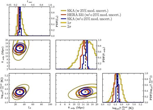
Analogous to Fig. 5, except here we show the impact of our assumed choice of a 25 per cent EoR modelling error, which dominates on large scales (see Fig. 2). Constraints from the SKA with the modelling error are shown in yellow, while those without any modelling error are shown in blue (SKA) and red (HERA). We see that under the optimistic assumption that we can perfectly characterize the EoR modelling uncertainties, the derived parameter constraints can be improved by a factor of a few (see Table 3).
We also list the corresponding constraints in Table 3. As expected, the resulting fractional errors are dramatically improved by a factor of 2–3 to 8.1/5.5, 7.2/8.1 and 1.4/0.9 per cent for HERA/SKA (for ζ0, Rmfp and log |$T^{\rm Feed}_{\rm vir}$|, respectively).
The fact that the parameter constraints improve dramatically and in a comparable manner for both HERA and the SKA shows that the redshift evolution of large-scale power dominates the constraining power for this EoR model. Unlike for narrow-band, single-z observations in Fig. 3, the additional leverage provided by small scales does not dramatically improve the parameter constraints if the redshift evolution of the large-scale power can be constrained. We caution however that this conclusion is dependent on the EoR model.
We also note that these values without the modelling error are in reasonable agreement with the roughly comparable12 constraints recovered by Pober et al. (2014), suggesting the Fisher matrix approach provides a reasonably accurate description of available constraints for this simple EoR parametrization.
TWO GALAXY POPULATIONS WITH MASS-DEPENDENT IONIZING EFFICIENCIES
In the previous section, we highlighted the strength of |$21$|CMMC at providing constraints on our model parameters from a simple single ionizing source population. However, physically we expect galaxy formation to be more complicated. Therefore, in this section, we consider a more flexible EoR model which allows for both a halo mass-dependent ionizing efficiency and multiple ionizing source populations.
Generalized five parameter EoR model
Our generalized EoR model contains a total of five parameters, the same three EoR parameters as described in Section 2.1 (ζ0, Rmfp and |$T^{\rm Feed}_{\rm vir}$|) and the two new power-law indices describing the mass-dependent ionizing efficiency, α and β. For our fiducial mock observation, we choose to adopt α = 4/3 and β = −1/3, both within the allowed range, α, β ∈ [ − 4/3, 10/3]. If instead we define equation (9) with respect to mass, these power-law indices become α = 2 and β = −1/2 (since |$M\propto T^{3/2}_{\rm vir}$|). Our specific choice of α and β for our fiducial model is purely illustrative, and allows a strong mass-dependent scaling for the feedback limited galaxies, with a flatter slope contribution from the high-mass galaxies. In the local Universe, observations show that for low-mass galaxies the star formation efficiency may increase with host halo mass, f⋆ ∝ M2/3 (Kauffmann et al. 2003). On the other hand, our framework also allows small-mass galaxies to have even higher ionizing efficiencies than the high-mass galaxies. Such models (e.g. Alvarez, Finlator & Trenti 2012) could be motivated by a much higher escape fraction in small galaxies (e.g. Wise et al. 2014). For our remaining EoR parameters, we adopt ζ0 = 70, |${\rm log}_{10}T^{\rm Feed}_{\rm vir} = 4.7$| and Rmfp = 15 Mpc.
Again, we provide an illustrative example of our generalized EoR model by constructing a schematic picture of the expected z = 8 UV luminosity function in Fig. 8 following the same approach as in Section 2.1. We convert our new critical feedback temperature, |$T^{\rm Feed}_{\rm vir}$| into a UV magnitude (total halo mass) of MUV = −13.7 (M ∼ 109.11 M⊙), and denote this and the atomic cooling threshold by the vertical dashed lines. For the massive (bright) galaxies, denoted by β = −1/3, we use the same fits to the UV luminosity function in Kuhlen & Faucher-Giguère (2012). As before, this fit for these bright galaxies can be translated to fesc ∝ M−0.18 (see the discussion in Section 3.1.1).
A schematic picture of the z = 8 non-ionizing UV luminosity function (blue curve) from our fiducial reionization model generalized to include two different source galaxy populations. First, above a critical temperature, |$T^{\rm Feed}_{\rm vir}$|, haloes are sufficiently massive to be weakly affected by internal feedback process (e.g. supernovae driven winds), whose efficiency we describe by the power-law index β. Between |$T^{\rm Feed}_{\rm vir}$| and a cooling threshold temperature of Tvir = 104 K, haloes are sufficiently large to cool and form galaxies; however, their ionizing efficiency is affected by internal feedback processes, described by a second power-law index α. Note that the model curve at |$T_{\rm vir} > T^{\rm Feed}_{\rm vir}$| is obtained from a power-law fit to the halo mass as a function of UV magnitude recovered from abundance matching, which we can use to imply that for our fiducial choice of β = −1/3 we roughly obtain the scaling, fesc ∝ M−0.18 (see the text for further discussions).
Constraints from combining multiple redshift observations
Given the increased parameter degeneracies in this generalized five parameter EoR model, we will focus only on multiple epoch observations of the 21 cm PS. As in Section 3.4, we assume three independent 1000 h observations of the 21 cm PS at z = 8, 9 and 10; however, only for HERA and the SKA. In Fig. 9, we show the recovered 1D marginalized PDFs for each of the five EoR model parameters from HERA (red curves) and SKA (blue curves) and in Fig. 10, we show the corresponding 2D joint marginalized likelihood contours and the resulting 1D PDFs of the IGM neutral fraction at each observed epoch. Finally, in Table 4, we report the recovered median values and the corresponding 16th and 84th percentiles of our EoR model parameters.
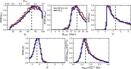
The marginalized 1D PDFs for each of the five reionization parameters (ζ0, Rmfp, α, β and |$T^{\rm Feed}_{\rm vir}$|) from our generalized EoR model containing two distinct ionizing galaxy populations for a combined 1000 h observation of the 21 cm PS across multiple redshifts (z = 8, 9 and 10). We consider two separate telescope designs, HERA (red) and the SKA (blue), and the vertical lines denote our fiducial input parameters (ζ0, Rmfp, α, β, |$T^{\rm Feed}_{\rm vir}$|) = (70, 15 Mpc, 4/3, −1/3, 4.7).
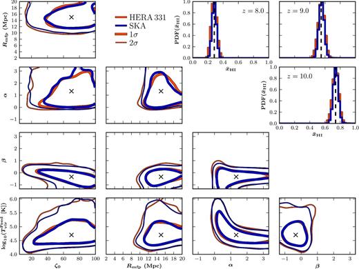
The 2D joint marginalized likelihood contours for our generalized five parameter EoR model (ζ0, Rmfp, α, β and |$T^{\rm Feed}_{\rm vir}$|) for a combined 1000 h observation of the 21 cm PS across multiple redshifts (z = 8, 9 and 10). We consider two separate telescope designs, HERA (red) and SKA (blue), crosses denote the fiducial model parameters and the 1σ and 2σ contours are shown as the thick and thin contours, respectively. Additionally, in the top-right corner we provide the one-dimensional PDFs of the recovered IGM neutral fraction for each individual redshift observation, with the vertical dashed line denoting the neutral fraction of the mock 21 cm PS observations, |$\bar{x}_{\mathrm{H\,{\small I}}{}} = 0.28$|, 0.55 and 0.74, respectively.
Summary of the median recovered values (and associated 16th and 84th percentile errors) for the five reionization parameters, ζ0, Rmfp, α, β and |$T^{\rm Feed}_{\rm vir}$| from the generalized EoR model (two ionizing galaxy populations) and the associated IGM neutral fraction, |$\bar{x}_{\mathrm{H\,{\small I}}{}}$|. We assume a total 1000 h integration time for each of the three different epoch observations of the 21 cm PS at z = 8, 9 and 10 for HERA and SKA. Our fiducial mock observation corresponds to (ζ0, Rmfp, α, β, |${\rm log}_{10}T^{\rm Feed}_{\rm vir}$|) = (70, 15 Mpc, 4/3, −1/3, 4.7) which results in an IGM neutral fraction of |$\bar{x}_{\mathrm{H\,{\small I}}{}} = 0.28$|, 0.55, 0.74 at z = 8, 9 and 10, respectively.
| Instrument | Parameter | |$\bar{x}_{\mathrm{H\,{\small I}}{}}$| | ||||||
|---|---|---|---|---|---|---|---|---|
| (multi-z) | ζ0 | Rmfp (Mpc) | α | β | log10|$(T^{\rm Feed}_{\rm vir})$| | z = 8 | z = 9 | z = 10 |
| HERA 331 | 68.28 ${{\scriptstyle {\begin{array}{c}
+20.27 \\
-25.96\end{array}}}}$ | 14.99 ${{\scriptstyle {\begin{array}{c}
+2.89 \\
-2.36\end{array}}}}$ | 1.10 ${{\scriptstyle {\begin{array}{c}
+1.28 \\
-0.72\end{array}}}}$ | -0.31 ${{\scriptstyle {\begin{array}{c}
+0.39 \\
-0.45\end{array}}}}$ | 4.74 ${{\scriptstyle {\begin{array}{c}
+0.42 \\
-0.22\end{array}}}}$ | 0.28 ${{\scriptstyle {\begin{array}{c}
+0.04 \\
-0.03\end{array}}}}$ | 0.55 ${{\scriptstyle {\begin{array}{c}
+0.04 \\
-0.04\end{array}}}}$ | 0.74 ${{\scriptstyle {\begin{array}{c}
+0.04 \\
-0.04\end{array}}}}$ |
| SKA | 70.20 ${{\scriptstyle {\begin{array}{c}
+18.62 \\
-25.68\end{array}}}}$ | 14.87 ${{\scriptstyle {\begin{array}{c}
+2.79 \\
-2.13\end{array}}}}$ | 1.11 ${{\scriptstyle {\begin{array}{c}
+1.33 \\
-0.70\end{array}}}}$ | -0.33 ${{\scriptstyle {\begin{array}{c}
+0.37 \\
-0.43\end{array}}}}$ | 4.73 ${{\scriptstyle {\begin{array}{c}
+0.44 \\
-0.21\end{array}}}}$ | 0.28 ${{\scriptstyle {\begin{array}{c}
+0.03 \\
-0.03\end{array}}}}$ | 0.55 ${{\scriptstyle {\begin{array}{c}
+0.03 \\
-0.03\end{array}}}}$ | 0.74 ${{\scriptstyle {\begin{array}{c}
+0.03 \\
-0.03 \end{array}}}}$ |
For the majority of these EoR parameters, we recover rather broad PDFs, noting mild to strong asymmetries emphasizing the strength of the degeneracies. This is to be expected with more model parameters. As an example, focusing on the α-|${\rm log}_{10}T^{\rm Feed}_{\rm vir}$| panel for a decreasing |$T^{\rm Feed}_{\rm vir}$| (increasingly narrower mass range for the feedback limited galaxies), any strong suppression (high α) can mimic the same behaviour as our fiducial model. This is due to the fact that for our assumed value of α = 4/3 the strong mass suppression in the ionizing efficiency only allows low-mass galaxies closest to |$T^{\rm Feed}_{\rm vir}$| to provide any meaningful contribution to reionization.
Despite these degeneracies, we are still able to recover meaningful constraints on these EoR parameters. For example, the contribution of low-mass galaxies to reionization as well as a well-defined feedback scale are picked up in the marginalized 1D |$T^{\rm Feed}_{\rm vir}$| PDFs. Such fundamental issues in galaxy formation are unlikely to be addressed with direct observations, even with JWST.
Quantitatively, both HERA and the SKA are able to recover median values for the five EoR parameters to within 5 per cent of their fiducial values with α being the exception (∼20 per cent). The corresponding percentile errors for α are additionally rather broad, however, this was to be expected from the qualitative analysis above (i.e. a strong mass dependence of α is hard to constrain due to the narrow range in mass of these galaxies which can contribute to reionization). Finally, from Fig. 10, we see that the PDFs of the IGM neutral fraction are tightly centred around the expected values from our fiducial model, and their quantitative errors are equivalent to our simple three parameter EoR model. This indicates that we have extracted all the available information from sampling the reionization history for both our 21 cm experiments. In principle, we could improve these constraints by (i) adding measurements of the 21 cm PS in additional bands (e.g. at z = 7); (ii) applying priors on to our EoR model parameters; (iii) considering alternative statistics of the 21 cm signal in combination with the 21 cm PS; or (iv) reducing the intrinsic modelling uncertainty.
It is important to note, that the discussion of the degeneracies and constraints of these EoR parameters is specific to our chosen fiducial model for the mock observation. Due to the sharp break in the power-law indices describing the two populations of ionizing galaxies and our choice for |$T^{\rm Feed}_{\rm vir}$|, the contribution to reionization from the high-mass (efficient star-forming) galaxy population can be relatively well constrained (as evident by the recovered PDF for β). Such a model is motivated by theoretical predictions of a sharp feedback scale (e.g. Finlator et al. 2011; Raičević et al. 2011). If however, we select a shallower break in the power-law indices, we effectively spread out the allowed range of masses of the ionizing galaxies (i.e. a shallower, positive α allows an increased contribution from the lower mass galaxies as they are not as efficiently suppressed). To illustrate this pessimistic case, in Fig. 11 we consider (ζ0, Rmfp, α, β, |$T^{\rm Feed}_{\rm vir}$|) = (30, 15 Mpc, 2/5, 1/15, 4.8). As expected, we now recover much broader PDFs. Most notably, with the shallower break in the power-law indices, it becomes increasingly difficult to constrain |$T^{\rm Feed}_{\rm vir}$| due to the smoother transition between the ionizing efficiency of the two galaxy populations. This is understandable, as in this model the two galaxy populations resemble a single population.
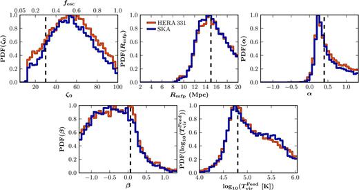
Same as Fig. 9, except now we consider an EoR model with a weaker break in the power-law indices. For this model, our EoR parameters are (ζ0, Rmfp, α, β, log |$T^{\rm Feed}_{\rm vir}$|) = (30, 15 Mpc, 2/5, 1/15, 4.8). As expected, reducing the amplitude of each power-law index and weakening the relative break between them, reduces the overall constraining power on all EoR model parameters.
CONCLUSION
The EoR is rich in astrophysical information, probing the nature of the first stars and galaxies, as well as their impact on the IGM. However, our current understanding of EoR astrophysics is poorly understood. Our understanding will rapidly improve in the near future with the detection of the cosmic 21 cm signal from a broad range of dedicated 21 cm experiments. However, we are faced with the fundamental question, what exactly can we learn from these observations?
To this end, we developed |$21$|CMMC,13 a new, massively parallel MCMC analysis tool specifically designed to recover constraints on any astrophysical parameters during the EoR from observations of the cosmic 21 cm signal. |$21$|CMMC utilizes existing astrophysical simulation codes and parameter estimation techniques to ensure its efficiency and flexibility. It combines the astrophysical parameter sampler cosmohammer (Akeret et al. 2013), calling the seminumerical 21 cm simulation code |$21$|CMFAST (Mesinger & Furlanetto 2007; Mesinger et al. 2011) at each point in the sampled EoR astrophysical parameter space. This allows sampling over 105 individual realizations of the cosmic 21 cm signal to recover robust EoR parameter constraints, without common assumptions of Gaussian errors.
Throughout this work, we have emphasized several key strengths of |$21$|CMMC, outlining its applicability to a broad range of studies of the 21 cm signal during the EoR. In summary, we
showed by utilizing a Bayesian MCMC framework, we can efficiently and accurately recover robust astrophysical constraints by recovering the marginalized 1D PDFs, irrespective of any model degeneracies. This removes the fundamental limitations and assumptions inherent in previous EoR astrophysical parameter studies such as sampling fixed grids (e.g. Choudhury & Ferrara 2005; Barkana 2009; Mesinger et al. 2012; Zahn et al. 2012), Fisher Matrix approaches (Pober et al. 2014) or simplistic analytic modelling of the EoR (Harker et al. 2012; Morandi & Barkana 2012; Patil et al. 2014);
highlighted that it is generalizable to any theoretical model of the EoR. We showcased two such models: (i) a popular, three parameter EoR model driven by a single population of star-forming galaxies characterized by a constant (mass-independent) ionizing efficiency; and (ii) a generalized five parameter EoR model containing two ionizing galaxy populations each characterized by a unique mass-dependent power-law ionizing efficiency;
highlighted the available constraining power from both single redshift and combining multiple redshift observations of the ionization 21 cm PS for three current and proposed 21 cm experiments, LOFAR, HERA and the SKA;
recovered for LOFAR/HERA/SKA fractional errors of 45.3/22.0/16.7, 33.5/18.4/17.8 and 6.3/3.3/2.4 per cent on the ionizing efficiency (escape fraction), mean free path of ionizing photons and the minimum halo mass hosting star formation from combining three independent 1000 h observations of the 21 cm PS at z = 8, 9 and 10 assuming no priors and a conservative noise estimate;
showed that by removing the EoR modelling uncertainty from our fiducial analysis, these constraints can be improved by up to a factor of a ∼few. This result motivates further work on characterizing EoR modelling errors in order to maximize science returns from second-generation instruments;
quantified the improvements in constraining power on the EoR parameters from accessing the additional information from the cosmic reionization history through the application of physically motivated priors on the IGM neutral fraction at the tail-end of reionization;
emphasized that |$21$|CMMC additionally allows for the inclusion of individual priors on the EoR model parameters motivated by current and upcoming observations and theoretical advances. Furthermore, while we have focused solely on the 21 cm PS, it is easily adaptable to consider any statistical measure of the cosmic 21 cm signal.
Finally, due its applicability to a broad range of EoR studies, |$21$|CMMC could be an important analysis tool for the 21 cm EoR community. For example, it can be used to quantify how foregrounds and other contaminants can hinder the recovery of EoR astrophysics. Moreover, it can serve to guide designs and observing strategies for current and future 21 cm experiments to maximize their scientific returns.
We thank the anonymous referee for their helpful suggestions. We are grateful to Jonathan Pober, Adrian Liu and Adam Lidz for valuable comments on a draft version of this manuscript. Additionally, we thank Jonathan Pober for making his telescope sensitivity code |$21$|cmsense publicly available and also Joel Akeret and Sebastian Seehars for the development and public release of cosmohammer.
|$21$|CMMC will be made available at http://homepage.sns.it/mesinger/21CMMC.html. Interested users can obtain a pre-release beta version by contacting the authors.
The ionization structure of these subgrid models of recombinations inside unresolved systems does not in fact directly translate to a constant, uniform value of Rmfp. These authors find that it takes a long time for cosmic H ii regions to approach the Strömgren limit, with their expansion only slowing more and more as reionization progresses. In other words, the mean free path (which is only defined in terms of the instantaneous recombination rate) is almost always larger than the actual size of the H ii regions (which depend on the cumulative number of recombinations), even at the late stages of reionization. The resulting ionization fields have a dearth of ionization structure on scales smaller than the instantaneous mean free path. Moreover, the spatial correlations between the sources and sinks of ionizing photons results in sizeable spatial and temporal variations in the mean free path. Nevertheless, an effective, uniform maximum horizon for ionizing photons of ∼10 Mpc can reproduce the 21 cm power spectra of the Sobacchi & Mesinger (2014) simulations to within tens of percent on relevant scales, at the epochs studied in that work |$0.25 \lesssim \bar{x}_{\mathrm{H\,{\small I}}{}} \lesssim 0.75$| (Sobacchi, private communication; Mesinger & Greig, in preparation). For historical context, we use the variable ‘Rmfp’ to denote this effective horizon set by subgrid recombinations, but caution that the actual mean free path is larger than this parameter, as discussed above.
These authors found a factor of 2.5 difference between their SKA and HERA designs for their estimated total sensitivity on a measurement of the 21 cm PS at z = 9.5. However, this factor was a result of a numerical error in their calculation of their SKA sensitivities. Accounting for this, their HERA design has in fact only a marginally reduced sensitivity relative to the SKA for their pessimistic and moderate foreground scenarios (Pober, private communication)
At present, |$21$|CMMC computes only co-evolving data cubes of the EoR. In future, we intend to improve the simulation pipeline to mimic a more realistic observational pipeline, taking into account several effects such as finite light-cones, foreground cleaning etc.
A like-to-like comparison is difficult for several reasons. First, these authors jointly combine four different epoch observations of the 21 cm PS compared to our three. Since instrument sensitivity increases with decreasing redshift, improved constraining power is available from their additional z = 7 observation (although it is not a significant improvement as three redshift measurements will have already strongly constrained the reionization history). Secondly, we consider only a 331 telescope antenna for HERA, unlike their 547 telescope design, while for the SKA there is the previously noted numerical error in their total sensitivities.
