


Abstract
We present the first public release of our generic neural network training algorithm, called SkyNet. This efficient and robust machine learning tool is able to train large and deep feed-forward neural networks, including autoencoders, for use in a wide range of supervised and unsupervised learning applications, such as regression, classification, density estimation, clustering and dimensionality reduction. SkyNet uses a ‘pre-training’ method to obtain a set of network parameters that has empirically been shown to be close to a good solution, followed by further optimization using a regularized variant of Newton's method, where the level of regularization is determined and adjusted automatically; the latter uses second-order derivative information to improve convergence, but without the need to evaluate or store the full Hessian matrix, by using a fast approximate method to calculate Hessian-vector products. This combination of methods allows for the training of complicated networks that are difficult to optimize using standard backpropagation techniques. SkyNet employs convergence criteria that naturally prevent overfitting, and also includes a fast algorithm for estimating the accuracy of network outputs. The utility and flexibility of SkyNet are demonstrated by application to a number of toy problems, and to astronomical problems focusing on the recovery of structure from blurred and noisy images, the identification of gamma-ray bursters, and the compression and denoising of galaxy images. The SkyNet software, which is implemented in standard ANSI c and fully parallelized using MPI, is available at http://www.mrao.cam.ac.uk/software/skynet/.
1 INTRODUCTION
In modern astronomy, one is increasingly faced with the problem of analysing large, complicated and multidimensional data sets. Such analyses typically include tasks such as: data description and interpretation, inference, pattern recognition, prediction, classification, compression, and many more. One way of performing such tasks is through the use of machine learning methods. For accessible accounts of machine learning and its use in astronomy, see, for example, MacKay (2003), Ball & Brunner (2010) and Way et al. (2012). Moreover, machine learning software easily used for astronomy, such as the python-based astroML package,1 or c-based Fast Artificial Neural Network Library (FANN2) have recently started to become available.
Two major categories of machine learning are: supervised learning and unsupervised learning. In supervised learning, the goal is to infer a function from labelled training data, which consist of a set of training examples. Each example has both ‘properties’ and ‘labels’. The properties are known ‘input’ quantities whose values are to be used to predict the values of the labels, which may be considered as ‘output’ quantities. Thus, the function to be inferred is the mapping from properties to labels. Once learned, this mapping can be applied to data sets for which the values of the labels are not known. Supervised learning is usually further subdivided into classification and regression. In classification, the labels take discrete values, whereas in regression the labels are continuous.
In astronomy, for example, using multifrequency observations of a supernova light curve (its properties) to determine its type (e.g. Ia, Ib, II, etc.) is a classification problem since the label (supernova type) is discrete (see, e.g. Karpenka, Feroz & Hobson 2013), whereas using the observations to determine (say) the energy output of the supernova explosion is a regression problem, since the label (energy output) is continuous. Classification can also be used to obtain a distribution for an output value that would normally be treated as a regression problem. This is demonstrated by Bonnett (2013) for measuring redshifts in Canada-France Hawaii Telescope Lensing Survey (CFHTLenS). A particularly important recent application of regression supervised learning in astrophysics and cosmology (and beyond) is the acceleration of the statistical analysis of large data sets in the context of complicated models. In such analyses, one typically performs many (|${\sim } 10^{4\text{--}6}$|) evaluations of the likelihood function describing the probability of obtaining the data for different sets of values of the model parameters. For some problems, in particular in cosmology, each such function evaluation can take up to tens of seconds, making the analysis very computationally expensive. By performing regression supervised learning to infer and then replace the mapping between model parameters and likelihood value, once can reduce the computation required for each likelihood evaluation by several orders of magnitude, thereby vastly accelerating the analysis (see, e.g. Fendt & Wandelt 2007; Auld et al. 2008a; Auld, Bridges & Hobson 2008b).
In unsupervised learning, the data have no labels. More precisely, the quantities (often termed ‘observations’) associated with each data item are not divided into properties (inputs) and labels (outputs). This lack of a ‘causal structure’, where the inputs are assumed to be at the beginning and outputs at the end of a causal chain, is the key difference from supervised learning. Instead, all the observations are considered to be at the end of a causal chain, which is assumed to begin with some set of ‘latent’ (or hidden) variables. The aim of unsupervised learning is to infer the number and/or nature of these latent variables (which may be discrete or continuous) by finding similarities between the data items. This then enables one to summarize and explain key features of the data set. The most common tasks in unsupervised learning include density estimation, clustering and dimensionality reduction. Indeed, in some cases, dimensionality reduction can be used as a pre-processing step to supervised learning, since classification and regression can sometimes be performed in the reduced space more accurately than in the original space.
As an astronomical example of unsupervised learning one might wish to use multifrequency observations of the light curves of a set of supernovae to determine how many different types of supernovae are contained in the set (a clustering task). Alternatively, if the data set also includes the type of each supernova (determined using spectroscopic observations), one might wish to determine which properties, or combination of properties, in the light curves are most important for determining their type photometrically (a dimensionality reduction task). This reduced set of property combinations could then be used instead of the original light-curve data to perform the supernovae classification or regression analyses mentioned above.
An intuitive and well-established approach to machine learning, both supervised and unsupervised, is based on the use of artificial neural networks (NNs), which are loosely inspired by the structure and functional aspects of a brain. They consist of a group of interconnected nodes, each of which processes information that it receives and then passes this product on to other nodes via weighted connections. In this way, NNs constitute a non-linear statistical data modelling tool, which may be used to represent complex relationships between a set of inputs and outputs, to find patterns in data, or to capture the statistical structure in an unknown joint probability distribution between observed variables. In general, the structure of an NN can be arbitrary, but many machine learning applications can be performed using only feed-forward NNs. For such networks the structure is directed: an input layer of nodes passes information to an output layer via zero, one, or many ‘hidden’ layers in between. Such a network is able to ‘learn’ a mapping between inputs and outputs, given a set of training data, and can then make predictions of the outputs for new input data. Moreover, a universal approximation theorem assures us that we can accurately and precisely approximate the mapping with an NN of a given form. A useful introduction to NNs can be found in MacKay (2003).
In astronomy, feed-forward NNs have been applied to various machine learning problems for over 20 years (see, e.g. Andreon et al. 1999, 2000; Longo, Tagliaferri & Andreon 2001; Tagliaferri et al. 2003a,b; Way et al. 2012). Nonetheless, their more widespread use in astronomy has been limited by the difficulty associated with standard techniques, such as backpropagation, in training networks having many nodes and/or numerous hidden layers (i.e. ‘large’ and/or ‘deep’ networks), which are often necessary to model the complicated mappings between the numerous inputs and outputs in modern astronomical applications.
In this paper, we therefore present the first public release of SkyNet: an efficient and robust NN training tool that is able to train large and/or deep feed-forward networks.3 SkyNet is able to achieve this by using a combination of the ‘pre-training’ method of Hinton, Osindero & Teh (2006) to obtain a set of network weights close to a good optimum of the training objective function, followed by further optimization of the weights using a regularized variant of Newton's method based on that developed for the MemSys software package (Gull & Skilling 1999). In particular, second-order derivative information is used to improve convergence, but without the need to evaluate or store the full Hessian matrix, by using a fast approximate method to calculate Hessian-vector products (Schraudolph 2002; Martens 2010). SkyNet is implemented in the standard ANSI c programming language and parallelized using MPI.4
We also note that SkyNet has already been combined with MultiNest (Feroz & Hobson 2008; Feroz, Hobson & Bridges 2009; Feroz et al. 2013), to produce the Blind Accelerated Multimodal Bayesian Inference (bambi) package (Graff et al. 2012), which is a generic and completely automated tool for greatly accelerating Bayesian inference problems (by up to a factor of ∼106; see, e.g. Bridges et al. 2011). MultiNest is a fully parallelized implementation of nested sampling (Skilling 2004), extended to handle multimodal and highly degenerate distributions. In most astrophysical (and particle physics) Bayesian inference problems, MultiNest typically reduces the number of likelihood evaluations required by an order of magnitude or more, compared to standard Markov chain Monte Carlo (MCMC) methods, but bambi achieves further substantial gains by speeding up the evaluation of the likelihood itself by replacing it with a trained regression NN. bambi proceeds by first using MultiNest to obtain a specified number of new samples from the model parameter space, and then uses these as input to SkyNet to train a network on the likelihood function. After convergence to the optimal weights, the network's ability to predict likelihood values to within a specified tolerance level is tested. If it fails, sampling continues using the original likelihood until enough new samples have been made for training to be performed again. Once a network is trained that is sufficiently accurate, its predictions are used in place of the original likelihood function for future samples for MultiNest. On typical problems in cosmology, for example, using the network reduces the likelihood evaluation time from seconds to less than a millisecond, allowing MultiNest to complete the analysis much more rapidly. As a bonus, at the end of the analysis the user also obtains a network that is trained to provide more likelihood evaluations near the peak if needed, or in subsequent analyses. With the public release of SkyNet, we now also make bambi publically available.5
The structure of this paper is as follows. In Section 2 we describe the general structure of feed-forward NNs, including a particular special case of such networks, called autoencoders, which may be used for performing non-linear dimensionality reduction. In Section 3 we present the procedures used by SkyNet to train networks of these types. SkyNet is then applied to some toy machine learning examples in Section 4, including a regression task, a classification task, and a dimensionality reduction task using autoencoders. We also apply SkyNet to the problem of classifying images of handwritten digits from the MNIST data base, which is a widely used benchmarking test of machine learning algorithms. The application of SkyNet to astronomical machine learning examples is presented in Section 5, including: a regression task to determine the projected ellipticity of a galaxy from blurred and noisy images of the galaxy and of a field star; a classification task, based on a simulated gamma-ray burst (GRB) detection pipeline for the Swift satellite (Gehrels et al. 2004), to determine if a GRB with given source parameters will be detected; and a dimensionality reduction task using autoencoders to compress and denoise galaxy images. Finally, we present our conclusions in Section 6.
2 NETWORK STRUCTURE
2.1 Feed-forward neural networks
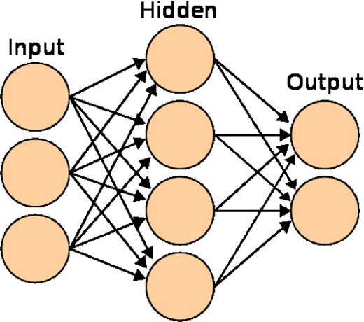
A 3-layer NN with 3 inputs, 4 hidden nodes, and 2 outputs. Image courtesy of Wikimedia Commons.
The weights and biases are the values we wish to determine in our training (described in Section 3). As they vary, a huge range of non-linear mappings from inputs to outputs is possible. In fact, a universal approximation theorem (Cybenko 1989; Hornik, Stinchcombe & White 1990) states that an NN with three or more layers can approximate any continuous function to some given accuracy, as long as the activation function is locally bounded, piecewise continuous, and not a polynomial (hence our use of sigmoid g(1), although other functions would work just as well, such as tanh ). By increasing the number of hidden nodes, one can achieve more accuracy at the risk of overfitting to our training data.
Other activation functions have also been proposed, such as the rectified linear function wherein g(x) = max{0, x} or the ‘softsign’ function where g(x) = .x/(1 + |x|). It has been argued that the former removes the need for pre-training (as described in Section 3.3; Glorot, Bordes & Bengio 2011) and serves as a better model of biological neurons. The ‘softsign’ is similar to tanh , but with slower approach to the asymptotes of ±1 (quadratic rather than exponential; Begstra et al. 2009; Glorot & Bengio 2010). Currently, SkyNet only utilizes the linear and sigmoid activation functions, but use of further options will be included in future releases of the code. Furthermore, other options for the connectivity of layers (e.g. pooling and convolution) are planned for future implementation.
2.2 Autoencoders
Autoencoders are a specific type of feed-forward NN containing one or more hidden layers, where the inputs are mapped to themselves, i.e. the network is trained to approximate the identity operation; when more than one hidden layer is used this is typically referred to as a ‘deep’ autoencoder. Such networks typically contain several hidden layers and are symmetric about a central layer containing fewer nodes than there are inputs (or outputs). A basic diagram of an autoencoder is shown in Fig. 2, in which the three inputs (x1, x2, x3) are mapped to themselves via three symmetrically arranged hidden layers, with two nodes in the central layer.
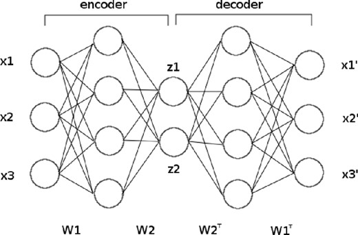
Schematic diagram of an autoencoder. The three input values are encoded to two feature variables. Pre-training (described in Section 3.3) defines the weight matrices W1 and W2.
An autoencoder can thus be considered as two half-networks, with one part mapping the inputs to the central layer and the second part mapping the central layer values to the outputs (which approximate as closely as possible the original inputs). These two parts are called the ‘encoder’ and ‘decoder’, respectively, and map either to or from a reduced set of ‘feature variables’ embodied in the nodes of the central layer (denoted by z1 and z2 in Fig. 2). These variables are, in general, non-linear functions of the original input variables. One can determine this dependence for each feature variable in turn simply by decoding (z1, 0, 0, …, 0), (0, z2, 0, …, 0), and so on, as the corresponding zi value is varied; in this way, for each feature variable, one obtains a curve in the original data space. Conversely, the collection of feature values (z1, z2, …, zM) in the central layer might reasonably be termed the feature vector of the input data. Autoencoders therefore provide a very intuitive approach to non-linear dimensionality reduction and constitute a natural generalization of linear methods such as principal component analysis (PCA) and independent component analysis (ICA), which are widely used in astronomy. Indeed, an antoencoder with a single hidden layer and linear activation functions may be shown to be identical to PCA (Sanger 1989). This topic is explored further in Section 4.3. It is worth noting that encoding from input data to feature variables can also be useful in performing clustering tasks; this is illustrated in Section 4.4.
Autoencoders are, however, notoriously difficult to train, since the objective function contains a broad local maximum where each output is the average value of the inputs (Erhan et al. 2010). Nonetheless, this difficulty can be overcome by the use of pre-training methods, as discussed in Section 3.3.
2.3 Choosing the number of hidden layers and nodes
An important choice when training an NN is the number of nodes in its hidden layers. The optimal number and organization into one or more layers has a complicated dependence on the number of training data points, the number of inputs and outputs, and the complexity of the function to be trained. Choosing too few nodes will mean that the NN is unable to learn the relationship to the highest possible accuracy; choosing too many will increase the risk of overfitting to the training data and will also slow down the training process. Using empirical evidence (Murtagh 1991) and theoretical considerations (Geva & Sitte 1992), it has been suggested that the optimal architecture for approximating a continuous function is one hidden layer containing 2N + 1 nodes, where N is the number of input nodes. Serra-Ricart et al. (1993) also find empirical support for this suggestion. Such a choice allows the network to model the form of the mapping function without unnecessary work.
In practice, it can be better to overestimate (slightly) the number of hidden nodes required. As described in Section 3, SkyNet performs basic checks to prevent overfitting, and the additional training time associated with having more hidden nodes is not a large penalty if an optimal network can be obtained in an early attempt. In any case, given a particular problem, the optimal network structure, both in terms of the number of hidden nodes and how they are distributed into layers, can be determined by comparing the correlation and error squared of different trained NNs; this is illustrated in Section 4.
3 NETWORK TRAINING
In training an NN, we wish to find the optimal set of network weights and biases that maximize the accuracy of the predicted outputs. However, we must be careful to avoid overfitting to our training data, which may lead to inaccurate predictions from inputs on which the network has not been trained.
The set of training data inputs and outputs (or ‘targets’), |$\mathcal {D} = \lbrace \boldsymbol {x}^{(k)},\boldsymbol {t}^{(k)}\rbrace$|, is provided by the user (where k counts training items). Approximately 75 per cent should be used for actual NN training and the remainder retained as a validation set that will be used to determine convergence and to avoid overfitting. This ratio of 3:1 gives plenty of information for training but still leaves a representative subset of the data for checks to be made.
3.1 Data whitening
It is prudent to ‘whiten’ the data before training a network. Whitening normalizes the input and/or output values, so that it easier to train a network starting from initial weights that are small and centred on zero. The network weights in the first and last layers can then be ‘unwhitened’ after training so that the network will be able to perform the mapping from original inputs to outputs.
One of these transforms may be chosen by the user if they wish to whiten the inputs of the training data. The whitening is normally performed separately on each input, but can be calculated across all inputs if they are related. The mean, standard deviation, minimum, or maximum would then be computed over all inputs for all training data items. The chosen whitening transform is also used for whitening the outputs. Since both transforms consist of subtracting an offset and multiplying by a scalefactor, they can easily be performed and reversed. To unwhiten network weights the inverse transform is applied, with the offset and scale determined by the source input node or target output node. Outputs for a classification network are not whitened since they are already just probabilities (see below).
3.2 Network objective function
3.2.1 Regression likelihood
3.2.2 Classification likelihood
3.3 Initialization and pre-training
The training of the NN can be started from some random initial state, or from a state determined from a ‘pre-training’ procedure discussed below. In the former case, the network training begins by setting random values for the network parameters, sampled from a normal distribution with zero mean and variance of 0.01 (this value can be modified by the user).
In the latter case, SkyNet makes use of the pre-training approach developed by Hinton et al. (2006), which obtains a set of network weights and biases close to a good solution of the network objective function. This method was originally devised with autoencoders in mind and is based on the model of restricted Boltzmann machines (RBMs). An RBM is a generative model that can learn a probability distribution over a set of inputs. It consists of a layer of input nodes and a layer of hidden nodes, as shown in Fig. 3. In this case, the map from the inputs to the hidden layer and then back is treated symmetrically and the weights are adjusted through a number of ‘epochs’, gradually reducing the reproduction error. To model an autoencoder, RBMs are ‘stacked’, with each RBM's hidden layer being the input for the next. The initial case is the NN's inputs to the first hidden layer; this is repeated for the first to second hidden layer and so on until the central layer is reached. The network weights can then be ‘unfolded’ by using the transpose for the symmetric connections in the decoding half to provide a decent starting point for the full training to begin. This is shown in Fig. 2, where the W1 and W2 weights matrices are defined by pre-training.
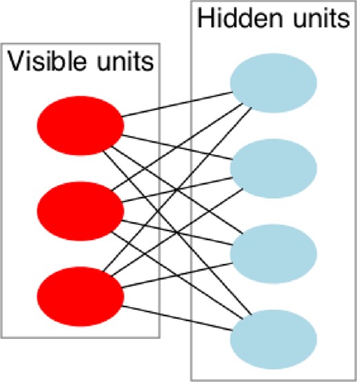
Diagram of an RBM with 3 visible nodes and 4 hidden nodes. Bias nodes are not shown. Image courtesy Wikimedia Commons.
The training is then performed using contrastive divergence (Carreira-Perpignan & Hinton 2005). This procedure can be summarized in the following steps, where sampling indicates setting the value of the node to 1 with the probability calculated and 0 otherwise.
Take a training sample |${\boldsymbol x}$| and compute the probabilities of the hidden nodes (their values using a sigmoid activation function) and sample a hidden vector |${\boldsymbol h}$| from this distribution.
Let |$g_{+} = {\boldsymbol x} \otimes {\boldsymbol h}$|, where ⊗ is used to indicate the outer product.
Using |${\boldsymbol h}$|, compute the probabilities of the visible nodes and sample |${\boldsymbol x}^\prime$| from this distribution. Resample the hidden vector from this to obtain |${\boldsymbol h}^\prime$|.
Let |$g_{-} = {\boldsymbol x}^\prime \otimes {\boldsymbol h}^\prime$|.
wi, j↦wi, j + r(g+ − g−) for some learning rate 0 < r ≤ 1.
More details can be found in Hinton et al. (2006) and Hinton & Salakhutdinov (2006) has useful diagrams and explanations.
This pre-training approach can also be used for more general feed-forward networks. All layers of weights, except for the final one that connects the last hidden layer to the outputs, are pre-trained as if they were the first half of a symmetric autoencoder. However, the network weights are not unfolded; instead the final layer of weights is initialized randomly as would have been done without pre-training. In this way, the network ‘learns the inputs’ before mapping to a set of outputs. This has been shown to greatly reduce the training time on multiple problems by Glorot & Bengio (2010) and Erhan et al. (2010).
We note that when an autoencoder is pre-trained, the activation function to the central hidden layer is made linear and the activation function from the final hidden layer to the outputs is made sigmoidal. General feed-forward networks that are pre-trained continue to use the original activation functions. Both of these are simply the default settings and the user has the freedom to alter them to suit his specific problem.
3.4 Optimization of the objective function
Once the initial set of network parameters has been obtained, either by assigning them randomly or through pre-training, the network is then trained (further) by iterative optimization of the objective function.
NN training then proceeds using an adapted form of a truncated Newton (or ‘Hessian-free’) optimization algorithm as described below, to calculate the step, |$\delta \boldsymbol {a}$|, that should be taken at each iteration. Following each such step, adjustments to α and σ may be made before another step is calculated. First, σ can be updated by multiplying it by a value c such that |$c^2 = \left.-2(\log \mathcal {L}+\log \mathcal {S})/M\right.$|. This serves to assure that at convergence, the χ2 value equals the number of unconstrained data points of the problem. Similarly, α is then updated such that the probability |$\Pr (\mathcal {D}\vert \alpha )$| is maximized for the current set of NN parameters |$\boldsymbol {a}$|. These procedures are described in detail by Gull & Skilling (1999, sections 2.3 and 2.6) and Hobson et al. (1998, section 3.6 and appendix B).
There are, however, some major practical difficulties with the standard Newton's method. First, the Hessian |${{\bf H}}$| of the log likelihood is not guaranteed to be positive semidefinite. Thus, even after the addition of the damping term |$\alpha {{\bf I}}$| derived from the log prior, the full Hessian |${{\bf B}}$| of the log posterior may also not be invertible. Secondly, even if |${{\bf B}}$| is invertible, the inversion is prohibitively expensive if the number of parameters is large, as is the case even for modestly sized NNs.
To address the first issue, we replace the Hessian |${{\bf H}}$| with a form of Gauss–Newton approximation |${{\bf G}}$|, which is guaranteed to be positive semidefinite and can be defined both for the regression likelihood (8) and the classification likelihood (10), respectively (Schraudolph 2002). In particular, the approximation used differs from the classical Gauss–Newton matrix in that it retains some second derivative information. Secondly, to avoid the prohibitive expense of calculating the inverse in (14), we instead solve (13) (with |${{\bf H}}$| replaced by |${{\bf G}}$| in |${{\bf B}}$|) for |$\delta \boldsymbol {a}$| iteratively using a conjugate-gradient algorithm, which requires only matrix–vector products |${{\bf B}}\boldsymbol {v}$| for some vector |$\boldsymbol {v}$|.
The combination of all the above methods makes practical the use of second-order derivative information even for large networks and significantly improves the rate of convergence of NN training over standard backpropagation methods.
It has been noted that this method for quasi-Newton second-order descent is equivalent to the first-order ‘natural gradient’ by Pascanu & Bengio (2013).
3.5 Convergence
As one might expect, as the optimization proceeds, there is a steady increase in the values of the posterior, likelihood, correlation, and negative of the error squared, evaluated both for the training and validation data. Eventually, however, the algorithm will begin to overfit, resulting in the continued increase of these quantities when evaluated on the training data, but a decrease in them when evaluated on the validation data. This divergence in behaviour is taken as indicating that the algorithm has converged and the optimization in terminated. The user may choose which of the four quantities listed above is used to determine convergence, although the default is to use the error squared, since it does not include the hyperparameters σ and α in its calculation and is less prone to problems with zeros than the correlation.
3.6 Optimizing network structure
We note that the correlation and the error-squared functions discussed above also provide quantitative measures with which to compare the performance of different network architectures, both in terms of the number of hidden nodes and how they are distributed into layers. As network size and complexity is increased, a point will be reached at which minimal or no further gains may be achieved in increasing correlation or reducing error squared. Therefore, any network architecture that can achieve this peak performance is equally well suited. In practice, we will wish to find the smallest or simplest network that does so as this minimizes the risk of overfitting and the time required for training.
3.7 Estimating the error on network outputs
After training a network, in particular a regression network, one may want to calculate the accuracy of the network's predicted outputs. A computationally cheap method of estimating this was suggested by MacKay (1995), whereby one adds Gaussian noise to the true outputs of the training data and trains a new network on this noisy data. After performing many realizations, the networks’ predictions will average to the predictions in the absence of the added noise. Moreover, the standard deviation of their predictions will provide a good estimate of the accuracy of the original network's predictions. Since one can train the new networks using the original trained network as a starting point, the re-training on noisy data is very fast. Additionally, evaluating the ensemble of predictions to measure the accuracy is not very computationally intensive as network evaluations are simple to perform and can be done in less than a millisecond. Explicitly, the steps of this method are as follows.
Start with the converged network with parameters |$\boldsymbol {a}^{\ast }$|, trained on the original data set |$D^{\ast } = \lbrace \boldsymbol {x}^{(k)},\boldsymbol {t}^{(k)}\rbrace$|. Estimate the noise on the residuals using |$\sigma ^2 = \sum _k [t^{(k)}-y(\boldsymbol {x}^{(k)},\boldsymbol {a}^{\ast })]^2/K$|.
Define a new data set D1 by adding Gaussian noise of zero mean and variance σ2 to the outputs (targets) in D*.
Train an NN on D1 using the parameters |$\boldsymbol {a}^{\ast }$| as a starting point. Training should converge rapidly as the new data set is only slightly different from the original. Denote the new network parameters by |$\boldsymbol {a}^1$|.
Repeat steps (ii) and (iii) multiple times to obtain an ensemble of networks with parameters |$\boldsymbol {a}^j$|.
Use each of the networks |$\boldsymbol {a}^j$| to make a prediction for a given set of inputs. The accuracy of the original network's outputs can be estimated as the standard deviation of the outputs of these networks.
In addition to these steps, SkyNet includes the option for the user to add random Gaussian offsets to the parameters |$\boldsymbol {a}^{\ast }$| before training is performed on the new data set (step iii). This offset will aid the training in moving the optimization from a potential local maximum in the posterior distribution of the network parameters, but the size of the offset must be chosen for each problem; for this, we recommend using a value s ≲ 1/α. We thus add noise to both the training data and the saved network parameters before training a new network whose posterior maximum will be near to, but not exactly the same as, the original networks.
This method may be compared with that described in Graff et al. (2012) for determining the accuracy of the NN predictions for the likelihood used in bambi. Although the method described here requires the overhead time of training additional networks, this is small compared the speed gains possible. Indeed, the new method's accuracy computations require less than a millisecond, as opposed to tenths of a second for the method used previously. Consequently, the faster method described here is now incorporated into our new public release version of bambi, leading to around two orders of magnitude increase in speed over that reported in Graff et al. (2012).
3.8 Parallelization with MPI
SkyNet is able to take advantage of parallel computation using MPI and thereby drastically reduce the computational time. As the calculations of likelihoods, gradients, and Hessian-vector products all require a summation over all training data points, this process can be distributed across many CPUs. By distributing the computational load over C CPUs, the time required to compute the next step of the algorithm is reduced by a factor of approximately C. Thus, total run time can be reduced by a factor of up to C. As not all processes involved with network training have been parallelized, a completely linear speed-up with the number of processors C is not attained. However, the speed-up gets closer to linearity with C as the amount of training data is increased; with larger data sets, training time is increasingly dominated by likelihood, gradient and Hessian-vector product calculations.
4 APPLICATIONS: TOY EXAMPLES
4.1 Regression
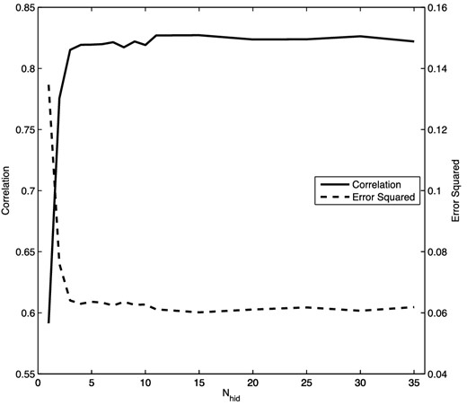
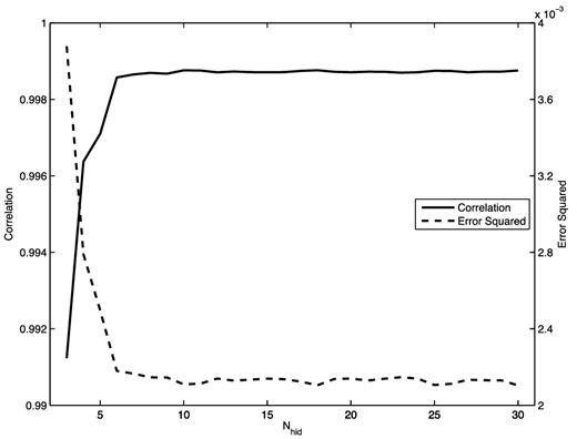
To perform the regression, the 200 data items (x, y) are divided randomly into 150 items for training and 50 for validation. For this simple problem, we use a network with a single hidden layer containing N nodes (we denote the full network by 1 + N + 1), and we whiten the input and output data using (4). The network was not pre-trained. The optimal value for N is determined by comparing the correlation and error squared for networks with different numbers of hidden nodes. These results are presented in Fig. 4, which shows that the correlation increases and the error squared decreases until we reach |$N\approx 6\text{--}7$| hidden nodes, after which both measures level off. Thus, adding additional nodes beyond this number does not improve the accuracy of the network. For the network with N = 7 hidden nodes, we obtain a correlation of greater than 99.3 per cent; a comparison of the true and predicted outputs in this case is shown in Fig. 5.
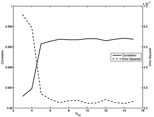
The correlation and error-squared values as a function of the number of hidden nodes N obtained from converged NNs with architecture 1 + N + 1 for the ramped sinc function regression problem.
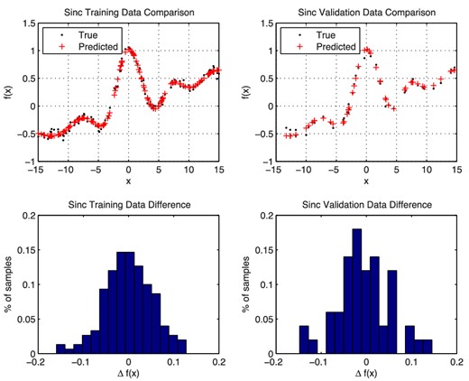
Comparisons of the true and predicted values obtained from the converged NN with architecture 1 + 7 + 1 on the training data (left) and validation data (right) for the ramped sinc function regression problem.
4.2 Classification
We now consider a toy classification problem based on the three-way classification data set created by Radford Neal6 for testing his own algorithms for NN training. In this data set, each of four variables x1, x2, x3, and x4 is drawn 1000 times from the standard uniform distribution |$\mathcal {U}[0,1]$|. If the two-dimensional Euclidean distance between (x1, x2) and (0.4, 0.5) is less than 0.35, the point is placed in class 0; otherwise, if 0.8x1 + 1.8x2 < 0.6, the class was set to 1; and if neither of these conditions is true, the class was set to 2. Note that the values of x3 and x4 play no part in the classification. Gaussian noise with zero mean and standard deviation 0.1 is then added to the input values.
Approximately 75 per cent of the data was used for training and the remaining 25 per cent for validation. We again use a network with a single hidden layer containing N nodes, and we whiten the input and output data using (4). The network was not pre-trained. The full network thus has the architecture 4 + N + 3, where the three output nodes give the probabilities (which sum to unity) that the input data belong to class 0, 1, or 2, respectively. The final class assigned is that having the largest probability.
The optimal value for N is again determined by comparing the correlation and error squared for networks with different numbers of hidden nodes. These results are shown in Fig. 6, from which we see that the correlation increases and the error squared decreases until we reach N ≈ 4 hidden nodes, after which both measures level off. For the network with N = 8 hidden nodes, a total of 87.8 per cent of training data points and 85.4 per cent of validation points were correctly classified. A summary of the classification results for this network is given Table 1. These results compare well with Neal's own original results and are similar to classifications based on applying the original criteria directly to data points that have noise added. Fig. 7 shows the data set and the true classifications.
The correlation and error squared of the converged NNs for the classification problem as a function of nodes in the single hidden layer.
Classification results for the converged NN with architecture 4 + 8 + 3 for the Neal data set.
| True class | Number | Predicted class (%) | |||
|---|---|---|---|---|---|
| 0 | 1 | 2 | |||
| Training data | 0 | 282 | 84.0 | 4.96 | 11.0 |
| 1 | 93 | 14.0 | 82.8 | 3.2 | |
| 2 | 386 | 7.0 | 1.3 | 91.7 | |
| Validation data | 0 | 99 | 75.7 | 6.1 | 18.2 |
| 1 | 19 | 21.1 | 78.9 | 0.0 | |
| 2 | 121 | 5.0 | 0.8 | 94.2 | |
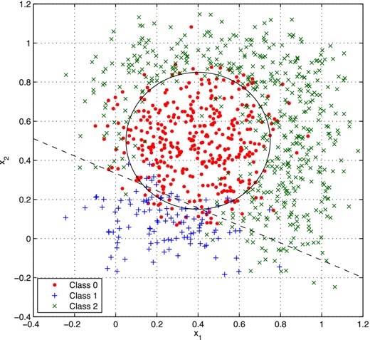
The full Neal data set (training and validation), showing the NN classifications (colour-coded) and the true criteria (solid and dashed lines) determining the classes of the data in the absence of noise.
4.3 Dimensionality reduction using autoencoders
Dimensionality reduction is a very common task in astronomy, which is usually performed using PCA (Kendall 1957) and its variants. In PCA, the eigenvalues and eigenvectors of the correlation matrix of the centred data (from which the mean has been subtracted) are found. The eigenvector directions define a new set of variables that are mutually orthogonal linear combinations of the original variables describing each data item. Dimensionality reduction is then achieved by keeping only those combinations corresponding to (a certain number of) the largest eigenvalues. PCA is limited, however, by its use of orthogonal projections and this has led to more recent interest in ICA, which still constructs linear combinations of the original variables, but relaxes the condition of orthogonality (see, e.g. Hyvärinen & Oja 2000). More specifically, ICA finds a set of directions such that the projections of the data on to these directions have maximum statistical independence, either by minimization of mutual information or maximization of non-Gaussianity.
As discussed in Section 2.2, antoencoders provide a natural generalization of PCA and ICA, and constitute an intuitive approach to non-linear dimensionality reduction that reduces to PCA in the special case of a single hidden layer and linear activation functions.
4.3.1 Multivariate Gaussian data
To provide a quick comparison of autoencoders and traditional PCA, we first consider two examples in which the data points are drawn from a single multivariate Gaussian distribution, as assumed in PCA, using a theoretical covariance matrix with given eigenvalues and eigenvectors. As a basic check, in both cases we perform the main PCA step of calculating the eigenvalues and eigenvectors of the sample covariance matrix of the resulting data points, and we find that they match those assumed very closely.
In our first example, we draw the data points (x1, x2) from a two-dimensional correlated Gaussian. For this simple case, we first train an autoencoder with a single hidden layer. Moreover, to effect a dimensionality reduction, we place just one node in the hidden layer, so the full network architecture is 2 + 1 + 2. Whitening of the input and output data using (5) was performed. Pre-training was also used as, even in such a very small autoencoder network (with a total of 7 network parameters), it is easy for the optimizer to fall into the large local maximum where each output is the average of the inputs.
Fig. 8(a) shows the original data and the curve traced out in the data space when one performs a decoding as the value of the feature variable z1 in the single central layer node is varied between the limits obtained when encoding the data. As one might expect, this curve approximates the eigenvector with larger eigenvalue of the covariance matrix of the data. The curve is not exactly a straight line because of the non-linearity of the activation function from the hidden layer to the output layer, and is influenced by the particular realization of the data analysed. It should be noted that dimensionality reduction is performed conversely, by (non-linearly) encoding each data point (x1, x2) to obtain the corresponding feature value z1 in the central layer node, rather than performing any PCA-like (linear) projection in the data space. The resulting error squared and correlation for the antoencoder are 0.476 and 90.5 per cent, respectively.
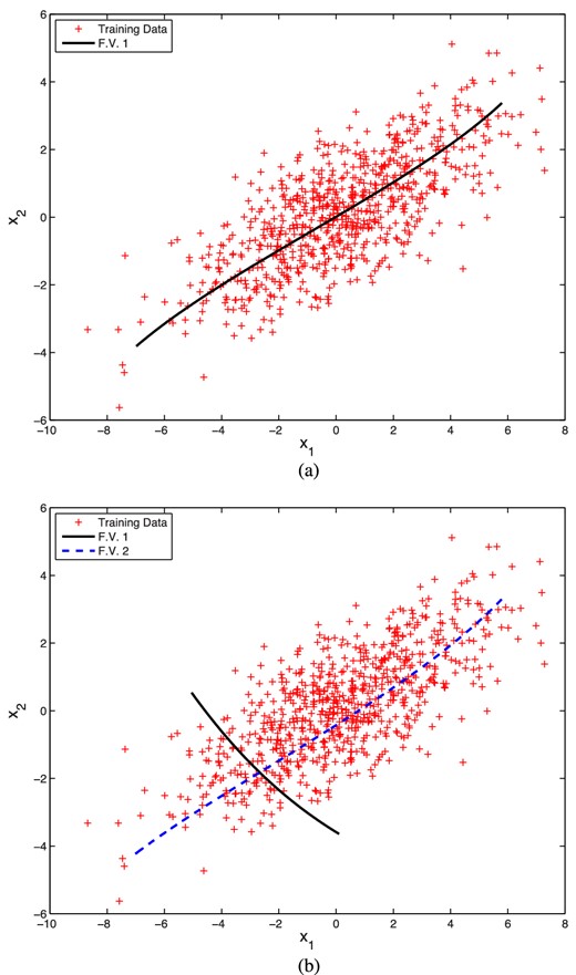
Original data points (red) drawn from a two-dimensional correlated Gaussian distribution, together with (a) the curve traced out by performing a decoding as one varies the single feature value z1 in the central layer of a trained autoencoder with architecture 2 + 1 + 2; and (b) two curves traced by performing a decoding as one varies the feature vectors (z1, 0) and (0, z2), respectively, in the central layer of a trained autoencoder with architecture 2 + 2 + 2. In both cases, the feature values are varied within the limits obtained when encoding the data.
To pursue the comparison with PCA further, we also train in a similar manner an autoencoder with two nodes in a single hidden layer, so the full network architecture is 2 + 2 + 2, although this is clearly no longer relevant for dimensionality reduction. Fig. 8(b) again shows the original data, together with the two curves traced out in the data space when one performs a decoding as one varies (between the limits obtained when encoding the data) the feature vectors (z1, 0) and (0, z2), respectively, in the central layer nodes. We see that, in the first case, one recovers a curve very similar to that shown in Fig. 8(a), whereas, in the second case, the curve approximates the eigenvector of the data covariance matrix having the smaller eigenvalue. As before, neither curve is exactly a straight line because of non-linearity of the activation function. Moreover, the curves do not intersect at right-angles, as would be the case for principal component directions. The resulting correlation and error squared for the antoencoder are 0.022 and 99.8 per cent, respectively. We note that the latter is very close to 100 per cent, as one would expect for this two-dimensional data set.
In our second example, we demonstrate the ability to determine the optimal number of nodes in the single hidden layer (and hence the optimal number of feature values) for an autoencoder, when redundant information is provided. To accomplish this, we draw data points from a three-dimensional correlated Gaussian, but then ‘rotate’ these points into five-dimensional space. Thus, each data point has the form (x1, x2, …, x5), but all the points lie on a three-dimensional hyperplane in this space. In a similar manner to above, we train autoencoders with architecture 5 + N + 5. As N is varied, the error squared and correlation of the resulting networks are given in Table 2. As expected, once three hidden nodes are used, the correlation is very close to 100 per cent, and adding more does not improve the results.
The error squared and correlation for autoencoder networks with architecture 5 + N + 5 applied to data points drawn from a three-dimensional correlated Gaussian distribution that are then ‘rotated’ into a five-dimensional space.
| Nhid | Error squared | Correlation % |
|---|---|---|
| 1 | 0.006 13 | 79.6 |
| 2 | 0.001 27 | 96.0 |
| 3 | 4.87 × 10⁻⁵ | 99.86 |
| 4 | 4.87 × 10⁻⁵ | 99.86 |
| 5 | 4.87 × 10⁻⁵ | 99.86 |
| Nhid | Error squared | Correlation % |
|---|---|---|
| 1 | 0.006 13 | 79.6 |
| 2 | 0.001 27 | 96.0 |
| 3 | 4.87 × 10⁻⁵ | 99.86 |
| 4 | 4.87 × 10⁻⁵ | 99.86 |
| 5 | 4.87 × 10⁻⁵ | 99.86 |
We note that, if desired, one can ‘rank’ the feature variables according to the amount by which they decrease the error squared or increase the correlation, which is analogous to ranking eigenvectors according to their eigenvalues in PCA.
4.3.2 Data distributed on a ring
where θ is drawn uniformly in the range [0.1π, 1.9π] and n is drawn from a Gaussian distribution with zero mean and standard deviation of 0.1; this example was originally presented in Serra-Ricart et al. (1993).
The data are plotted as the light blue points in Fig. 9 (top). Although the noiseless data are fully determined by the single parameter θ, it is clear that a linear dimensionality reduction method, such as PCA, would be unable to represent this data set accurately in a single component. Indeed, the dominant principal component would lie along a straight, horizontal (symmetry) line passing through the point (0.5, 0.5), as is easily verified in practice. Projections on to this direction clearly do not distinguish between data points having the same x1-coordinate, but lying on opposite sides of this symmetry line. As we will now show, however, it is possible to represent this data set well using just a single variable, by taking advantage of the non-linearity of an antoencoder.
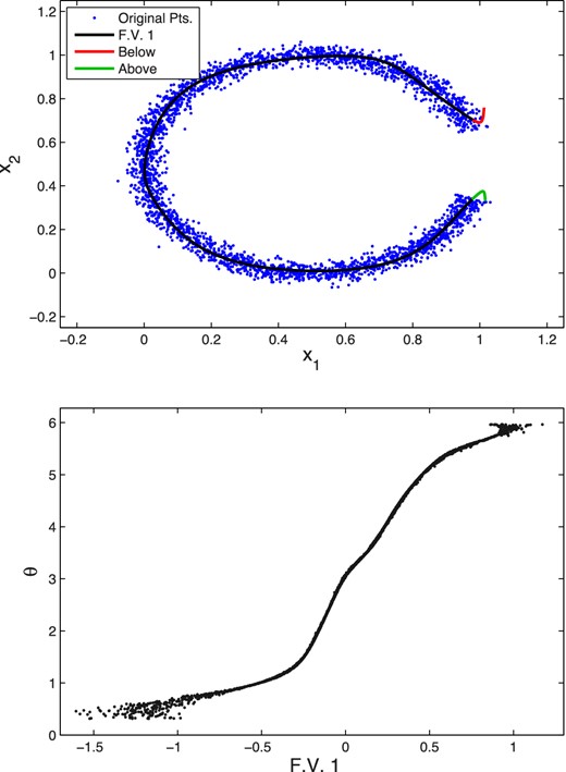
Top: original data points (light blue) and the curve (black) traced out by performing a decoding as one varies (between the limits obtained when encoding the data) the single feature value z1 in the central layer of a trained autoencoder with architecture 2 + 13 + 1 + 13 + 2. The curve traced out when z1 is allowed to vary below (above) the range encountered in training is shown in red (green). Bottom: the true angle θ of the training data points versus their encoded feature values.
In this slightly more challenging example, we train an autoencoder with three hidden layers, again with a single node in the central layer to perform a dimensionality reduction. Thus, the full network architecture is 2 + N + 1 + N + 2. Whitening of the input and output data was applied using (5), and the network was pre-trained. The optimal value for N is determined by comparing the correlation and error squared for networks with different numbers of hidden nodes. These results are shown in Fig. 10, which shows that optimal performance is reached for N ≳ 10, beyond which no significant improvement results from adding further hidden nodes.
The correlation and error-squared values as a function of the number of hidden nodes N obtained from converged autoencoder with architecture 2 + N + 1 + N + 2 for the data on a ring problem.
The results obtained for the antoencoder with architecture 2 + 13 + 1 + 13 + 2 are shown in Fig. 9. The top panel shows the curve (in black) traced out by performing a decoding as one varies (between the limits obtained when encoding the data) the single feature value z1 in the central layer of a trained autoencoder with architecture 2 + 13 + 1 + 13 + 2; this clearly follows the ring structure very closely. The curve traced out when z1 is allowed to vary below (above) the range encountered in training is shown in red (green). One sees that each of these curves extend a short distance into the gap in the ring, with one curve extending at either end of the gap. Conversely, the bottom panel shows the encoded feature value obtained as compared to the true angle θ of the input data. We see that, as expected, there is a strong and monotonic relationship between these two variables.
4.3.3 Data distributed in multiple Gaussian modes
In this example, we again consider a two-dimensional case in which the data are drawn from a distribution very different to a single multivariate Gaussian, but, rather than simulating a long, curving degeneracy, we focus here on a distribution possessing multiple modes. In particular, the data are generated from the sum of four equal Gaussian modes, each having a standard deviation of 0.1 in both the x1 and x2 directions, with means of (0.25, 0.25), (0.25, 0.75), (0.75, 0.25), and (0.75, 0.75), respectively; this example was also originally presented in Serra-Ricart et al. (1993).
The data are plotted as the light blue points in Fig. 11 (top). In this case it is not intuitively obvious to what extent the data can be represented using a single variable. It is once again clear, however, that a linear dimensionality reduction method, such as PCA, would be unable to represent this data set accurately in a single component. Indeed, in this case, the two principal directions lie along diagonal (symmetry) lines at ±45°, passing through the point (0.5, 0.5), and (in theory) have equal eigenvalues, so either direction can be used to perform the dimensionality reduction. Projection on to the line at +45° (say) will clearly not distinguish between any two data points that lie on any given line perpendicular to that direction, thereby conflating data points in modes 1 and 4 in the figure. Thus, the resulting histogram of projected values for the data points will contain only three (broad) peaks (see Serra-Ricart et al. 1993). As we now show, however, it is possible to distinguish all four modes using just a single variable, if one again makes use of the non-linear nature of autoencoders.
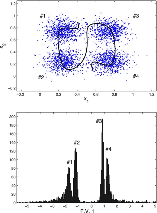
Top: original data points (light blue) and the curve (black) traced out by performing a decoding as one varies (between the limits obtained when encoding the data) the single feature value z1 in the central layer of a trained autoencoder with architecture 2 + 30 + 1 + 30 + 2. Bottom: histogram of the encoded feature values obtained from the input data; four separate peaks are visible, corresponding to the four Gaussian modes as labelled.
We again train an autoencoder with architecture 2 + N + 1 + N + 2, using whitening of the input with (5), and pre-training. The optimal value for N is determined by comparing the correlation and error squared for networks with different numbers of hidden nodes. Investigating values for N between 3 and 30, we find that N = 30 performed best by a small margin. The results from this network are shown in Fig. 11. The top panel shows the curve (in black) traced out by performing a decoding as one varies (between the limits obtained when encoding the data) the single feature value z1 in the central layer of a trained autoencoder; this curve traces out a path through the centre and outskirts of all four modes, each of which corresponds to a distinct range of feature values. This is illustrated in the bottom panel, which shows the histogram of the encoded feature values obtained from the data set. The histogram contains four clear peaks, each corresponding to one of the modes in the original data distribution. By setting appropriate threshold values on this feature variable, we can classify the points as belonging to each of the modes with a 97.83 per cent accuracy (classifying based on the raw x1 and x2 values yields only a slightly better accuracy of 98.85 per cent).
4.4 MNIST handwriting recognition
The MNIST data base of handwritten digits is a subset of a larger collection available from National Institute for Standards and Technology (NIST). It consists of 60 000 training and 10 000 validation images of handwritten digits. Each digit has been size-normalized and centred in a 28 × 28 pixel grey-scale image. The images are publicly available online,7 along with more information on the generation of the data set and results from previous analyses by other researchers. This data set has become a standard for testing of machine learning algorithms. Some sample digits are shown in Fig. 12. The learning task is to identify correctly the digit written in each image. Although this may be an easy task for a human brain, it is quite a challenging machine learning application.
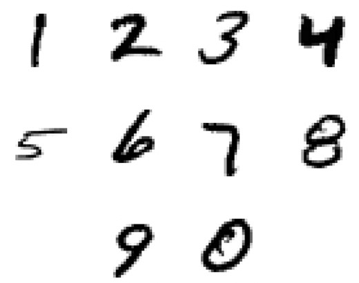
Sample handwritten digits from the MNIST data base.
4.4.1 Direct classification
Several classification networks of varying complexity were trained on this problem. In all cases, pre-training was used for any hidden layers and all inputs were whitened using the transformation (5). Each network has 28 × 28 = 784 inputs (corresponding to the grey-scale image size) and 10 outputs (one for each digit). The class (digit) assigned to each image was that having the highest output probability.
The results obtained are summarized in Table 3, where the error rates, defined as the fraction incorrectly classified, are those calculated on the set of validation images. We note that some of these networks are large and deep, but are nonetheless well trained using SkyNet. These results may be compared with those referenced on the MNIST website, which yield error rates as low as 0.35 per cent (Ciresan et al. 2010) but more typically between 1 and 5 per cent (LeCun et al. 1998).
Error rates for classification networks with different architectures, trained to identify handwritten digits in grey-scale images from the MNIST data base. All networks have 784 inputs and 10 outputs.
| Hidden layers | Error rate (%) |
|---|---|
| 0 | 8.08 |
| 100 | 4.15 |
| 250 | 3.00 |
| 1000 | 2.38 |
| 300 + 30 | 2.83 |
| 500 + 50 | 2.62 |
| 1000 + 300 + 30 | 2.31 |
| 500 + 500 + 2000 | 1.76 |
| Hidden layers | Error rate (%) |
|---|---|
| 0 | 8.08 |
| 100 | 4.15 |
| 250 | 3.00 |
| 1000 | 2.38 |
| 300 + 30 | 2.83 |
| 500 + 50 | 2.62 |
| 1000 + 300 + 30 | 2.31 |
| 500 + 500 + 2000 | 1.76 |
4.4.2 Dimensionality reduction and classification
A dimensionality reduction of the MNIST data was also performed. In particular, two large and deep autoencoder networks were trained, one with hidden layers 1000 + 300 + 30 + 300 + 1000 (called AE-30) and the other with hidden layers 1000 + 500 + 50 + 500 + 1000 (called AE-50); both networks have 784 inputs and outputs, corresponding to the image size. Thus, the dimensionality reduction to 30 or 50 feature variables, respectively, represents a significant data compression. The AE-30 network was able to obtain an average total error squared of only 4.64 and AE-50 obtained an average total error squared of 3.29. These values are comparable to those obtained in Hinton & Salakhutdinov (2006). Thus, despite reducing the dimensionality of the input data used from 784 pixels to 30 or 50 non-linear feature variables, these reduced basis sets retain enough information about the original images to reproduce them to within small errors. This also demonstrates that SkyNet is capable of training large and deep autoencoder networks.
As mentioned previously, dimensionality reduction is sometimes used as a prelude to a supervised-learning task such as classification, since the latter can sometimes be performed just as accurately (or sometimes more so) in the reduced space as in the original data space. To illustrate this approach, using each of AE-30 and AE-50, all the training images were passed through the autoencoder to obtain the (30 or 50) encoded feature values for each image. These feature values (rather than the original images) were then used to train a classification network (with just 30 or 50 input nodes, respectively, and 10 output nodes) to identify the handwritten digits. The resulting error rates are listed in Table 4, for networks with different numbers of hidden layers and nodes. In particular, comparing with Table 3, we see that the resulting classifications are nearly as accurate as the best-performing network trained on the full images, despite reducing the dimensionality of the input data from 784 pixels to 30 or 50 non-linear feature variables, and reducing the number of classification network parameters by several orders of magnitude.
Error rates for classification networks with different architectures, trained on autoencoder feature values to identify handwritten digits from the MNIST data base. For AE-30 (AE-50), all the classification networks have 30 (50) inputs and 10 outputs.
| Autoencoder | Classification hidden layers | Error rate (%) |
|---|---|---|
| AE-30 | 0 | 9.57 |
| 10 | 6.39 | |
| 30 | 3.03 | |
| 100 + 50 + 10 | 2.55 | |
| AE-50 | 0 | 8.68 |
| 10 | 6.61 | |
| 50 | 2.65 | |
| 100 + 50 + 10 | 2.71 |
| Autoencoder | Classification hidden layers | Error rate (%) |
|---|---|---|
| AE-30 | 0 | 9.57 |
| 10 | 6.39 | |
| 30 | 3.03 | |
| 100 + 50 + 10 | 2.55 | |
| AE-50 | 0 | 8.68 |
| 10 | 6.61 | |
| 50 | 2.65 | |
| 100 + 50 + 10 | 2.71 |
4.4.3 Dimensionality reduction and clustering
Finally, a massive dimensionality reduction to just two feature variables was performed on the images by training a very large and deep autoencoder, with hidden layers 1000 + 500 + 250 + 2 + 250 + 500 + 1000 (and 784 inputs and outputs). As expected, this network is significantly less able to reproduce the original images, having an average total error squared of 31.0, but has the advantage that one can plot the two feature values obtained for each of the images to provide a simple illustration of clustering.
Such a scatterplot is shown in Fig. 13 for the 10 000 validation images, where the points are colour-coded according to the true digit contained in each image; this figure may be compared with fig. 3B in Hinton & Salakhutdinov (2006). We see that there is some significant overlap between digits with similar shapes, but that some digits do occupy distinct regions of the parameter space (particularly 1 in the top right, some 0s in the bottom right, and many examples of 2 in the middle right).
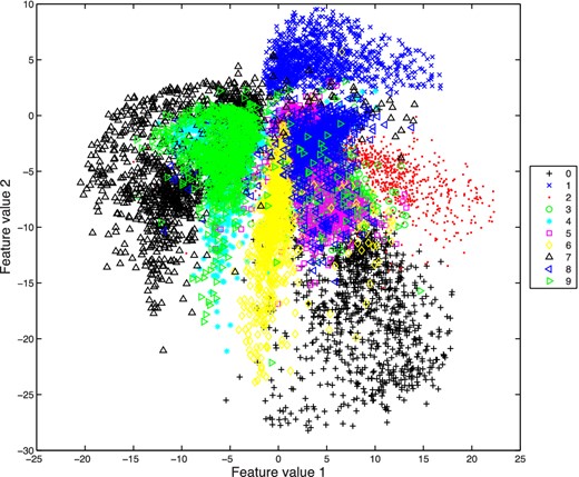
Scatterplot of the two feature variables for the 10 000 validation images from the MNIST data base, obtained using the encoding half 784 + 1000 + 500 + 250 + 2 of a symmetric autoencoder.
4.5 Comparison with FANN library
In this section, we perform a simple comparison between SkyNet and an alternative algorithm for training an NN. The case we use is the simple sinc problem from Section 4.1 and we compare against the FANN library. This is an NN library that has been developed over several years and thus has more features and interfaces than implemented thus far for SkyNet. However, the training is performed via standard backpropagation techniques which are first order in nature.
Training on the exact same sinc data with one hidden layer containing 7 nodes, we found that FANN's optimal predictions and run time were equivalent to those of SkyNet. However, FANN performed approximately an order of magnitude more steps in parameter space to reach this solution (meaning an individual step was similarly faster) and had no feature to prevent overfitting had a larger NN been trained (uses only target error and maximum number of steps). Furthermore, while running multiple times with SkyNet produces similar run time and results consistently, FANN run times varied greatly and often did not converge to the same result. Lastly, FANN requires the user to create their own ‘main’ function in c (or another language) to setup the network to be trained, read in data, perform training, and save the network. By comparison, SkyNet seeks to make these functions easier for the user by asking only for an input settings file and formatted data. The additional functionality can be implemented in future releases while a useful and simple tool is provided now.
5 APPLICATIONS: ASTROPHYSICAL EXAMPLES
5.1 Regression: Mapping Dark Matter challenge
The Mapping Dark Matter (MDM) challenge was presented in www.kaggle.com as a simplified version of the GREAT10 Challenge (Kitching et al. 2011). In this problem, each data item consists of two 48 × 48 grey-scale images of a galaxy and a star, respectively. Each pixel value in each image is drawn from a Poisson distribution with mean equal to the (unknown) underlying intensity value in that pixel. Moreover, both images have been convolved with the same, but unknown, point spread function. The learning task is, for each pair of images, to predict the ellipticities e1 and e2 (defined below) of the underlying true galaxy image, and thus constitutes a regression problem. The training data set contains 40 000 image pairs and the challenge data set contains 60 000 image pairs. A sample galaxy and star image pair is shown in Fig. 14. During the challenge, the solutions for the validation data set were kept secret and participating teams submitted their predictions. Further details about the challenge and descriptions of the top results can be found in Kitching et al. (2012).
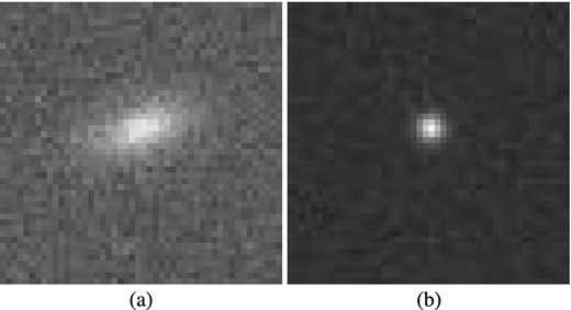
Example image pair of (a) galaxy and (b) star from the MDM Challenge; each image contains 48 × 48 grey-scale pixels.
5.1.1 Galaxy image model
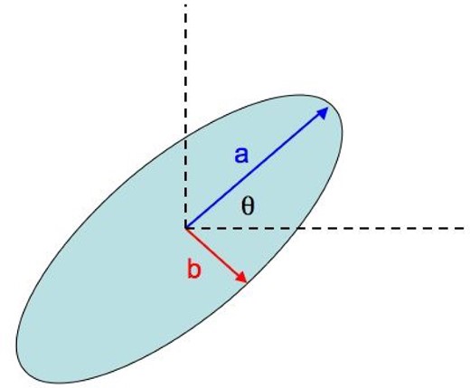
Definition of the underlying galaxy image ellipse parameters used in the MDM Challenge. Image from http://www.kaggle.com/c/mdm/.
5.1.2 Results
We use SkyNet to train several regression networks, each of which takes the galaxy and star images as inputs and produces estimates of the true galaxy ellipticities as outputs. Following the approach used in the original challenge, the quality of a network's predictions are measured by the root mean squared error (RMSE) of its predicted ellipticities over the challenge data set of 60 000 pairs of images. Clearly, better predictions result in lower values of the RMSE.
The size of the data set meant that training large networks was very computationally expensive. Therefore, for this demonstration, we train only relatively small networks, but used three different data sets: (i) the full galaxy and star images; (ii) the full galaxy image and a centrally cropped star image; and (iii) the full galaxy image alone. Of the training data provided, consisting of 40 000 image pairs, 75 per cent were used for training the networks [without pre-training and whitening using transformation (5)] and the remaining 25 per cent were used for validation. The RMSE values for trained networks of different architecture, evaluated on the challenge data set, are given in Table 5.
RMSE on ellipticity predictions for networks with different architectures, evaluated on the 60 000 image pairs of the MDM Challenge. All networks have two outputs: the galaxy ellipticities e1 and e2.
| Data set | Hidden layers | RMSE |
|---|---|---|
| Full galaxy and star images | 0 | 0.022 4146 |
| (48 × 48 × 2 = 4608 inputs) | 2 | 0.018 6944 |
| 5 | 0.018 4237 | |
| 10 | 0.018 2661 | |
| Full galaxy and cropped star images | 0 | 0.017 5578 |
| (48 × 48 + 24 × 24 = 2880 inputs) | 2 | 0.017 6236 |
| 5 | 0.017 5945 | |
| 10 | 0.017 4997 | |
| 50 | 0.017 2977 | |
| 50+10 | 0.017 1719 | |
| Full galaxy image only | 0 | 0.023 4740 |
| (48 × 48 = 2304 inputs) | 2 | 0.023 4669 |
| 5 | 0.023 6508 | |
| 10 | 0.022 6440 |
The RMSE values obtained even for the naive first approach of using the full data set (i) as inputs are quite good; for comparison, the standard software package SExtractor (Bertin & Arnouts 1996) produced an RMSE score of 0.086 2191 on this test data and the UWQM method scores 0.185 5600. One see from Table 5 that increasing the number of hidden nodes beyond two does improve the network accuracy, but only very slowly.
The NN results can, however, be improved more easily simply by reducing the number of inputs without affecting the information content, for example by cropping the star images to the central 24 × 24 pixels to yield data set (ii). This simple change increases the accuracy of the ellipticity predictions, thereby lowering the RMSE. Increasing the number of nodes in a single hidden layer, or adding an extra hidden layer, does yield improving predictions, although the rate of improvement is quite gradual. Nonetheless, this indicates that more complex networks could further improve the accuracy of the ellipticity predictions. The best result obtained for the networks investigated, with an RMSE of 0.017 1719, compares well with the competition winners, who achieved an RMSE of 0.015 0907 (Kitching et al. 2012) using a mixture of methods that included NNs. We note that our score, produced using an immediate ‘out-of-the-box’ application of SkyNet that involves no specialized data processing, would have placed us in 32nd place out of 66 teams that entered the challenge.
We see from Table 5, however, that reducing the number of inputs further by removing the star images altogether leads to a significant increase in the RMSE. This is to be expected since the absence of the star images does not allow for the NN to infer the point spread function sufficiently well to predict the underlying galaxy ellipticities accurately.
Finally, we note that all of our results could potentially be improved further by fitting profiles to the images and using the parameters of these fits for training, which would reduce the number of inputs by about two orders of magnitude. Alternatively, one could train an autoencoder to dimensionally reduce each image into a set of feature variables; this would again vastly reduce the number of network inputs also potentially alleviate the effect of noise in the images. Such investigations are, however, postponed to a future publication.
5.2 Classification: identifying gamma-ray bursters
Long GRBs are almost all indicators of core-collapse supernovae from the deaths of massive stars. The ability to determine the intrinsic rate of these events as a function of redshift is essential for studying numerous aspects of stellar evolution and cosmology. The Swift space telescope is a multiwavelength detector that is currently observing hundreds of GRBs (Gehrels et al. 2004). However, Swift uses a complicated combination of over 500 triggering criteria for identifying GRBs, which makes it difficult to infer the intrinsic GRB rate. Indeed, most studies approximate the Swift trigger algorithm by a single detection threshold, which can lead to biases in inferring the intrinsic GRB rate as a function of redshift.
To investigate this issue further, a recent study by Lien et al. (2014) performed a Monte Carlo analysis that generated a mock sample of GRBs, using the GRB rate and luminosity function of Wanderman & Piran (2010), and processed them through an entire simulated Swift detection pipeline, applying the full set of Swift trigger criteria, to determine which GRBs would be detected. It was found that the resulting measured GRB rate as a function of redshift followed very closely that of the true Swift GRB set described in Fynbo et al. (2009); this finding is consistent with both the mock GRB sample and the simulated trigger pipeline being good approximations to reality. This analysis was, however, quite computationally expensive, since determining if each GRB is detected by Swift requires over a minute on a single CPU.
5.2.1 Form of the classification problem
Our goal here is to replace the simulated Swift trigger pipeline with a classification NN, which (as we will see) can determine in just a few microseconds whether a given GRB is detected. To this end, we use as training data a pre-computed mock sample of 10 000 GRBs from Lien et al. (2014). In particular, we divide this sample randomly into ∼4000 for training, ∼1000 for validation, and the final ∼5000 as a blind test set on which to perform our final evaluations. For each GRB we use 13 inputs: the GRB total luminosity, redshift, and energy peak, together with the arrival bin at the Swift detector, bin size of the light curve in the emitting frame, α and β parameters for the GRB's Band function spectrum, background intensity in four different energy ranges (15–25, 15–50, 25–100, and 50–350 keV), angle of arrival at the detector, and total GRB flux. The two softmaxed outputs correspond to probabilities (which sum to unity) for the class 0, that the GRB is not detected, and for the class 1, that the GRB is detected. In our analysis, we will focus on the probability for class 1.
Different NN architectures were trained on these data and it was found that NNs with hidden layer configurations of 50, 100 + 30, and 300 + 100 + 30 all performed equally well on the classification task. Thus results presented in this section are those from the network with hidden layers 100 + 30 applied to the blind set of ∼5000 GRBs.
5.2.2 Results
In Fig. 16 we plot the actual and expected completeness and purity. It is clear that the actual and expected curves lie on top of one another with only minimal differences. Thus, without knowing the true classifications of the GRBs as detected or not, we can set pth to obtain the desired completeness and purity levels for the final sample.
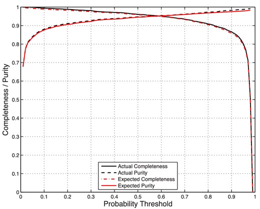
Actual and expected values for the completeness and purity as a function of probability threshold, pth. The expected curves are very accurate predictors of the actual ones.
With this information, we can also plot the actual and expected receiver operating characteristic (ROC) curves (see, e.g. Fawcett 2006). The ROC curve originated in signal detection theory and is a reliable way of choosing an optimal threshold value as well as comparing binary classifiers. The ROC curve plots the true positive rate (identical to completeness and also equal to the Neyman–Pearson ‘power’ of a test) against the false positive rate (also known as contamination and the Neyman–Pearson type-I error rate) as a function of the threshold value.9 A perfect classifier will have an ROC curve that connects (0, 0) to (0, 1) and then (1, 1), whereas a random classifier will yield an ROC curve that is the diagonal line connecting (0, 0) and (1, 1) directly. In general, the larger the area underneath an ROC curve, the more powerful the classifier.
From Fig. 17, we can see that the expected and actual ROC curves for an NN classifier are very close, with small deviations occurring only at very low false positive rates; it should be noted that here the actual ROC curve is better than the expected one. The curves also indicate that this test is quite powerful at predicting which GRBs will be detected by Swift.
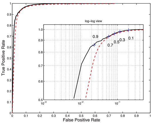
Actual (black solid) and expected (dashed red) ROC curves for an NN classifier that predicts whether a GRB will be detected by Swift. The curve traces true versus false positive rates as the probability threshold varies, as illustrated on the inset log–log plot.
Using the completeness, purity, and ROC curves, one can make a decision as to appropriate value of pth to use. One may require a certain level of completeness, regardless of false positives, or we may require a minimal level of contamination in the final sample. Alternatively, one can use the ROC curve to derive an optimal value for pth. For example, one can use the pth value where the ROC curve intersects with the diagonal line connecting (0, 1) and (1, 0), or where the line from the point (1, 0) intersects the ROC curve at right angles. From either of these criteria, we conclude that pth = 0.5, the original naive choice, is a near-optimal threshold value.
Using pth = 0.5, we now wish to determine how well the GRB detection rate with respect to redshift is reproduced, since this relationship is key to deriving scientific results. In Fig. 18, we show the event counts as a function of redshift for both our NN classifier and the original simulated Swift trigger pipeline. It is clear that the two sets of counts agree very well. In the bottom part of the figure, we calculate a measure of the error within each redshift bin by computing |$(N_{\rm t}-N_{\rm p})/\sqrt{N_{\rm t}}$|, where Nt is the ‘true’ number of GRBs detected by the full simulated Swift pipeline, and Np is the number obtained using our classification NN. As the original detection counting is essentially a Poissonian process, its intrinsic normalized error will remain within [−1, 1] for most bins, and we can see that error introduced by the NN similarly does not exceed this magnitude.
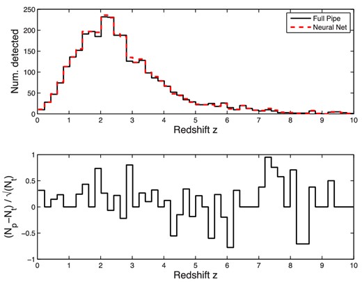
Top: comparison of the detected GRB event counts obtained using the full simulated Swift trigger pipeline and our classification NN. Bottom: normalized error between the two counts.
We note that networks used to obtain these results were trained in a few CPU hours and thereafter can make an accurate determination of whether a GRB will be detected by Swift in just a few microseconds, instead of the minutes of computation time required by the full simulated Swift trigger pipeline.
5.3 Dimensionality reduction: compressing galaxy images
In astronomical data analysis, the raw data set often contains a great deal of redundant information. Simply put, there are usually many more pixels in an astronomical image than there are distinct features to be identified in the object being imaged, so that not all pixels are independent measures of structure. If we are able to compress the data by removing these redundancies and instead quantify only the distinct features present, then one can be more efficient in subsequent analyses. One way of finding these features in the data and performing compression – and denoising – is through the use of autoencoders. As we have already shown, autoencoders are able to represent non-linear features in a data set and reduce the number of variables used to describe it to a value closer to the intrinsic dimensionality of the data.
5.3.1 Image compression and denoising
Our previous analysis, presented in Section 5.1, for measuring galaxy ellipticities from the MDM Challenge data set images provides a good example. The original galaxy images each contain 2304 pixels, but these are clearly not all independent measurements. Additionally, even the cropped star images each contain 576 non-independent pixels. With an autoencoder, we can compress both of these images by two orders of magnitude, from thousands of input variables to just tens, from which one can then measure ellipticities.
To perform the compression, autoencoders with a single hidden layer were trained, since these images contain relatively few features and simpler networks require less time to train. Pre-training was used in all examples. The input data were the 2880 pixels of each galaxy and its accompanying (cropped) star. Since the noise in each pixel is Poissonian, we report in Table 6 not only the RMSE on the autoencoder outputs, but also the RMSE normalized by the original pixel value. The values listed in Table 6 correspond to the mean values obtained for the collection of images comprising the MDM training data set. The values obtained from one image to another are mutually consistent, but when the autoencoder has 10 or more nodes in the hidden layer the image-to-image variations are significantly larger than the differences between the means. One sees from Table 6 that only a slight improvement is observed when using 10 or more hidden nodes. Indeed, taking into account image-to-image variation, the predictions by the larger networks are statistically indistinguishable from those of the smaller ones. We can therefore represent the images well with just 10 feature values. If we consider the original construction of the images, each galaxy can be represented by 4 parameters (two ellipticities, a position angle and an amplitude) and each star by 2 parameters (a radius for the point spread function and an amplitude). This means that, without noise, only 6 parameters are needed to describe the images completely. This is reflected by the ability of our autoencoder to perform the ‘majority’ of the fit with just 5 features. Additional features produce more marginal decreases in the RMSE as they are now fine-tuning and/or fitting for the noise in the data.
The mean RMSE values for autoencoder reconstructions of galaxy and cropped star images from the MDM Challenge data set. Pixel values range from 0 to 255. The normalized RMSE has had the errors divided by the square root of the original pixel value that was to be reconstructed.
| Hidden nodes | RMSE | Norm. RMSE |
|---|---|---|
| 1 | 9.09 | 0.955 |
| 2 | 8.83 | 0.936 |
| 3 | 8.66 | 0.922 |
| 5 | 8.50 | 0.909 |
| 10 | 8.44 | 0.904 |
| 30 | 8.43 | 0.903 |
| 50 | 8.42 | 0.901 |
| 100 | 8.38 | 0.897 |
| Hidden nodes | RMSE | Norm. RMSE |
|---|---|---|
| 1 | 9.09 | 0.955 |
| 2 | 8.83 | 0.936 |
| 3 | 8.66 | 0.922 |
| 5 | 8.50 | 0.909 |
| 10 | 8.44 | 0.904 |
| 30 | 8.43 | 0.903 |
| 50 | 8.42 | 0.901 |
| 100 | 8.38 | 0.897 |
By looking at pixel-to-pixel comparisons, one finds that a large part of the error is coming from the fainter pixels, which are, for the most part, distinctly external to the galaxy. Therefore, the galaxy itself is being described even more accurately than the numbers presented indicate. A plot of this comparison for a typical galaxy/star pair is shown in Fig. 19, with the corresponding original (input) and reconstructed (output) images shown in Fig. 20.
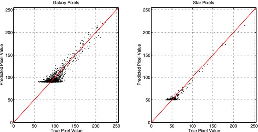
A pixel-by-pixel comparison for a typical galaxy/star image pair between original and autoencoder reconstructed images. We can see the larger errors occurring at smaller true pixel values associated with the background. This used an autoencoder with a single hidden layer of 10 nodes.
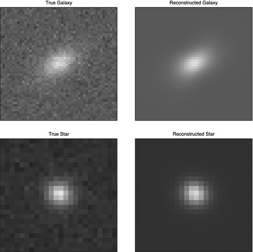
Comparison of original (input) and reconstructed (output) galaxy and star images for an autoencoder with a single hidden layer of 10 nodes. This example is the same as that shown in Fig. 19.
We can illustrate the nature of the feature vectors constructed by the network by decoding the central layer values (1, 0, 0, …), (0, 1, 0, …), etc. of our autoencoder, which has 10 hidden nodes, to obtain the corresponding 10 output images. We plot these images in Fig. 21 for the galaxy/star example shown in Fig. 20. Some shape features can be clearly seen, although the grey-scale has been reversed for these images to see them as brighter structures. This reversal can be accounted for by the network assigning the original features negative weights and a positive bias.

Features vectors obtained by decoding (1, 0, 0, …), (0, 1, 0, …), etc. in the central layer of an autoencoder with 10 central layer nodes. Shown are the extracted (a) galaxy and (b) star features. The grey-scale has been reversed on the actual values.
5.3.2 Estimating ellipticities with compressed data
Having trained the autoencoders, we now investigate using the compressed feature values, rather than original images, to determine the ellipticities of the galaxies. Since the number of inputs has been decreased from 2880 to 10–100, we can use more and larger hidden layers in our regression network and the analysis will still take less time to run. Results on training regression networks with many different configurations are given in Table 7.
RMSE values for galaxy ellipticity predictions using the compressed feature values as inputs. Various compressions and regression network sizes were used.
| # Features | Hidden layers | RMSE |
|---|---|---|
| 5 | 10 | 0.022 316 |
| 30 | 0.022 534 | |
| 100 | 0.022 015 | |
| 30 + 10 | 0.025 472 | |
| 100 + 30 | 0.025 165 | |
| 10 | 10 | 0.016 802 |
| 30 | 0.016 237 | |
| 100 | 0.016 296 | |
| 30 + 10 | 0.017 028 | |
| 100 + 30 | 0.017 869 | |
| 30 | 10 | 0.016 559 |
| 30 | 0.016 927 | |
| 100 | 0.016 608 | |
| 30 + 10 | 0.017 312 | |
| 100 + 30 | 0.017 351 | |
| 50 | 10 | 0.017 056 |
| 30 | 0.017 056 | |
| 100 | 0.016 769 | |
| 30 + 10 | 0.016 492 | |
| 100 + 30 | 0.016 629 | |
| 100 | 10 | 0.019 459 |
| 30 | 0.019 561 | |
| 100 | 0.019 596 | |
| 30 + 10 | 0.019 750 | |
| 100 + 30 | 0.019 949 |
These results show that the extra information given to the regression networks trained on 100 feature values from the autoencoder acted as a disadvantage in predicting the galaxy ellipticities. For networks trained on 50 or 30 features, however, the accuracies of the predicted ellipticities were better even than those obtained using the full original images in some cases. This demonstrates the power of being able to eliminate redundant information and noise, and thereby improve the accuracy of the analysis. We also observe that adding unnecessary complexity to the NN structure makes it more difficult for the algorithm to find the global maximum.
This same method for dimensionality reduction – which also eliminates noise – before performing measurements can clearly be applied to a wide range of other astronomical applications. Examples include classification of supernovae by type, or measurements of galaxies and stars by their spectra.
6 CONCLUSIONS
We have described an efficient and robust NN training algorithm, called SkyNet, which we have now made freely available for academic purposes. This generic tool is capable of training large and deep feed-forward networks, including autoencoders, and may be applied to supervised and unsupervised machine learning tasks in astronomy, such as regression, classification, density estimation, clustering and dimensionality reduction. SkyNet employs a combination of (optional) pre-training followed by iterative refinement of the network parameters using a regularized variant of Newton's optimization algorithm that incorporates second-order derivative information without the need even to compute or store the Hessian matrix. Linear and sigmoidal activation functions are provided for the user to choose between. SkyNet adopts convergence criteria that naturally prevent overfitting, and it also includes a fast algorithm for estimating the accuracy of network outputs.
We first demonstrate the capabilities of SkyNet on toy examples of regression, classification, and dimensionality reduction using autoencoder networks, and then apply it to the classic machine learning problem of handwriting classification for determining digits from the MNIST data base. In an astronomical context, SkyNet is applied to: the regression problem of measuring the ellipticity of noisy and convolved galaxy images in the MDM Challenge; the classification problem of identifying gamma-ray bursters that are detectable by the Swift satellite; and the dimensionality reduction problem of compressing and denoising images of galaxies. In each case, the straightforward use of SkyNet produces networks that perform the desired task quickly and accurately, and typically achieve results that are competitive with machine learning approaches that have been tailored to the required task.
Future development of SkyNet will expand upon many of the current features and introduce new ones. We are working to include more activation functions (e.g. tanh , softsign, and rectified linear), pooling of nodes, convolutional NNs, diversity in outputs (i.e. mixing regression and classification), and more robust support of recursive NNs. This is all in addition to further improving the speed and efficiency of the training algorithm itself. However, SkyNet in its current state is already a useful tool for performing machine learning in astronomy.
The authors thank John Skilling for providing very useful advice in the early stages of algorithm development. We also thank Amy Lien for providing the data used in Section 5.2. This work utilized three different high-performance computing facilities at different times: initial work was performed on COSMOS VIII, an SGI Altix UV1000 supercomputer, funded by SGI/Intel, HEFCE and PPARC, and the authors thank Andrey Kaliazin for assistance; early work also utilized the Darwin Supercomputer of the University of Cambridge High Performance Computing Service (http://www.hpc.cam.ac.uk/), provided by Dell Inc. using Strategic Research Infrastructure Funding from the Higher Education Funding Council for England; later work utilized the Discover system of the NASA Center for Climate Simulation at NASA Goddard Space Flight Center. PG is currently supported by a NASA Postdoctoral Fellowship from the Oak Ridge Associated Universities and completed a portion of this work while funded by a Gates Cambridge Scholarship at the University of Cambridge. FF is supported by a Research Fellowship from the Leverhulme and Newton Trusts.
SkyNet may also be used to train recurrent NNs (see, e.g. Mandic & Chambers 2001), but its application to such networks will be discussed in a future work.
A version of SkyNet parallelized for GPUs using CUDA is currently in development.
It is worth noting that, in terms of conditional probabilities, completeness is simply |$\Pr (\mbox{classified as detected}|\mbox{detected})$|, purity is its Bayes theorem complement |$\Pr (\mbox{detected}|\mbox{classified as detected})$|, and contamination is |$\Pr (\mbox{classified as detected}|\mbox{not detected})$|.
