


Abstract
We present a new approach for modelling galaxy/halo bias that utilizes the full non-linear information contained in the moments of the matter density field, which we derive using a set of numerical simulations. Although our method is general, we perform a case study based on the local Eulerian bias scheme truncated to second order. Using 200 N-body simulations covering a total comoving volume of 675 h−3 Gpc3, we measure several two- and three-point statistics of the halo distribution to unprecedented accuracy. We use the bias model to fit the halo–halo power spectrum, the halo–matter cross-spectrum and the corresponding three bispectra for wavenumbers in the range 0.04 ≲ k ≲ 0.12 h Mpc−1. We find that the constraints on the bias parameters obtained using the full non-linear information differ significantly from those derived using standard perturbation theory at leading order. Hence, neglecting the full non-linear information leads to biased results for this particular scale range. We also test the validity of the second-order Eulerian local biasing scheme by comparing the parameter constraints derived from different statistics. Analysis of the halo–matter cross-correlation coefficients defined for the two- and three-point statistics reveals further inconsistencies contained in the second-order Eulerian bias scheme, suggesting it is too simple a model to describe halo bias with high accuracy.
1 INTRODUCTION
The clustering statistics of the galaxy distribution contain a wealth of information about the cosmological model. However, in the absence of a robust theory for galaxy formation, extracting this information can only be achieved in part. In practice, to do this requires us to assume a specific phenomenological relationship between the density field of galaxies and that of the underlying matter, more commonly referred to as galaxy bias. Whilst still incomplete, our leading theories of galaxy formation, do provide a great deal of insight about the distribution of galaxies. For instance they predict that galaxies should only reside in dark matter haloes and be strongly associated with the distribution of substructures (for a detailed review of galaxy formation see Mo, van den Bosch & White 2010). This greatly simplifies our ability to construct a phenomenological model for the galaxy distribution on large scales: it should be closely related to a weighted average of the dark matter halo overdensities (e.g. Smith, Scoccimarro & Sheth 2007).
There are a number of detailed analytical approaches for characterizing the bias of dark matter haloes with respect to the mass distribution. However, it has yet to be determined which model provides the most accurate description of galaxy bias. In the simplest method, the local Eulerian bias model (hereafter LEB), one assumes that the overdensities of the biased tracers can be written as some function of the matter density field at the same location. If both densities are smoothed over the patch scale R, then the biased field may be written as a Taylor-series expansion (Fry & Gaztanaga 1993). If one considers sufficiently large patches, then high-order corrections are guaranteed to be small and the series may be truncated after a finite number of terms.
Halo-clustering predictions of the LEB expressed in terms of standard perturbation theory (hereafter SPT, for a review see Bernardeau et al. 2002) have been examined in numerous works (Scoccimarro et al. 2001; Smith et al. 2007; Guo & Jing 2009; Manera & Gaztañaga 2011; Roth & Porciani 2011; Chuen Chan & Scoccimarro 2012; Pollack, Smith & Porciani 2012). One of the results to emerge from these studies is that, when the model is applied to halo counts within finite volumes of linear size R, the coefficients of the bias expansion show a running with the ‘cell’ size. However, halo-clustering statistics such as the n-point correlation functions (or the corresponding n-spectra) do not contain any smoothing scale and should not depend on R. There has been much debate in the literature on how to reconcile these seemingly contrasting results.
This has led some to discuss an ‘effective’ or ‘renormalized’ bias approach where the scale dependence of the bias coefficients is compensated by the contribution of small-scale perturbations in the matter density (Heavens, Matarrese & Verde 1998; McDonald 2006; Schmidt, Jeong & Desjacques 2013). Whilst such a scheme may be plausible (Jeong & Komatsu 2009; Smith, Hernández-Monteagudo & Seljak 2009), the development of a unique renormalization method is still ongoing, especially for dynamically evolved configurations in Eulerian space. On the other hand, it was recently proposed by Chuen Chan & Scoccimarro (2012) that the bias parameters obtained by counting haloes within cells of size R are only relevant for describing perturbations of wavenumber k ≃ 0.8/R in the halo distribution. While there is no challenge to their argument when analysing power spectrum data, it does present a complication when using higher order statistics such as the bispectrum. In order to interpret the galaxy bispectrum one would be required to compute bias coefficients separately for each configuration of wavevectors. This approach appears somewhat cumbersome to implement.
Currently, most observational analyses of galaxy clustering assume that galaxy bias can be described by the truncated LEB and that the statistical properties of the non-linear matter density field can be modelled using SPT. To leading order in the perturbations, this requires only one bias parameter for two-point statistics of the tracers and two parameters for three-point statistics. Present-day galaxy surveys, however, do not cover enough comoving volume to accurately sample the spatial scales at which tree-level results provide an accurate description of galaxy clustering. The presence of rare large-scale structures, for instance, significantly alters the measurements of three-point statistics (e.g. Nichol et al. 2006). On smaller scales, where data are more robust, dynamical non-linearities pose a serious challenge to the models. Adopting the simplified LEB+SPT model may therefore generate systematic errors and thus influence the characterization of the bias or the estimation of the cosmological parameters.
The LEB truncated to second order is the standard workhorse for studying three-point statistics of galaxy clustering. Its predictions to leading perturbative order have been used to interpret measurements from the two-degree field (2dF) galaxy redshift survey (Verde et al. 2002; Jing & Börner 2004; Wang et al. 2004; Gaztañaga et al. 2005), the Sloan Digital Sky Survey (SDSS; Kayo et al. 2004; Hikage et al. 2005; Pan & Szapudi 2005; Kulkarni et al. 2007; Nishimichi et al. 2007; McBride et al. 2011a,b; Marín 2011; Guo et al. 2014), and the WiggleZ Dark Energy Survey (Marín et al. 2013). In our previous study (Pollack et al. 2012), we demonstrated that, in order to robustly model three-point statistics with the LEB, one must necessarily have an accurate model for the clustering statistics of the non-linear matter density on the relevant scales. This is imperative to recover the correct values of the bias parameters in controlled numerical experiments. Therefore, it is not surprising that past investigations based on the LEB+SPT model reached inconsistent conclusions. For example, studying the galaxy bispectrum on scales 0.1 < k < 0.5 h Mpc−1, Verde et al. (2002) concluded that 2dF galaxies are unbiased tracers of the mass distribution. On the other hand, using the complete 2dF sample, Gaztañaga et al. (2005) found strong evidence for non-linear biasing from the analysis of the three-point correlation function with triangle configurations that probe separations between 9 and 36 h−1 Mpc (see also Jing & Börner 2004; Wang et al. 2004).
In this paper, we build upon our past experience and present a general method to model the clustering of biased tracers of the mass distribution on mildly non-linear scales k < 0.1 h Mpc−1. This is key to extend studies of galaxy clustering to smaller spatial separations where observational data are less uncertain. Our method relies on using N-body simulations to measure the relevant statistics for the clustering of the underlying mass distribution. Related approaches have been presented by Sigad, Branchini & Dekel (2000) and Szapudi & Pan (2004) for galaxy counts in cells (see also Pan & Szapudi 2005 for an application to correlation functions). We apply our general framework to the modelling of n-point clustering statistics of non-linear, Eulerian, locally biased tracers. In our framework, bias parameters run with the patch scale R. We address the running of the bias by treating the filter scale as a nuisance parameter to be marginalized over. The major advantage of our scheme is that we exactly recover the matter polyspectra used in the bias model at every order. The only truncation necessary in the model is the choice as to what level to truncate the bias expansion, and this may be selected by the data in a Bayesian model comparison. We test our modelling framework up to quadratic order in the local bias expansion (as commonly done in recent observational studies), for the power and bispectra of haloes and their cross-spectra with matter measured from a large ensemble (200 realizations) of measurements from a series of large Λ cold dark matter (ΛCDM) N-body simulations. This ensemble of simulations resolves the haloes that should host luminous red galaxies over a total comoving volume of 675 h−3 Gpc3, and so provides us with a very stringent statistical test ground for our model.
The sections are organized as follows. In Section 2 we set our mathematical notation and introduce the LEB. The numerical simulations used in this work are briefly described in Section 3 and used in Section 4 to measure several statistical quantities for the matter and halo distributions. In Section 5 we use Bayesian statistics to estimate the free parameters of the LEB and describe our main results. Finally, in Sections 6 and 7 we further discuss our findings and present our conclusions.
2 A NEW FRAMEWORK FOR MODELLING THE CLUSTERING OF BIASED TRACERS
2.1 General formalism
The smoothing scale must therefore be considered as a free parameter of the model, and so it must be either determined by fitting a set of data or marginalized over.
In previous studies, the functions |${\mathcal {P}}_{(l,m)}$| and |${\mathcal {B}}_{(l,m,n)}$| have been modelled through the use of a combination of perturbation theory and semi-empirical models. In Pollack et al. (2012) we recovered these functions exactly from an N-body simulation and demonstrated that they are essential to measure the bias parameters in an unbiased way. We will revisit these issues in Sections 4 and 5.
2.2 Case study: biasing to second order
3 N-BODY SIMULATIONS
In order to test the LEB and also to determine the covariance matrices of the various spectra we have simulated 200 realizations of a flat ΛCDM cosmological model. The specific cosmological parameters that we have adopted are {σ8 = 0.8, Ωm = 0.25, Ωb = 0.04, h = 0.7, ns = 1.0} where σ8 is the variance of linear mass fluctuations in top-hat spheres of radius R = 8 h−1 Mpc; Ωm and Ωb are the matter and baryon density parameters; h is the dimensionless Hubble parameter in units of 100 km s−1 Mpc−1; and n is the power-law index of the primordial density power spectrum. Our adopted values were inspired by the results from the Wilkinson Microwave Anisotropy Probe experiment (Komatsu et al. 2009).
All of the N-body simulations were run using the publicly available Tree-PM code gadget-2 (Springel 2005). This code was used to follow with high accuracy the non-linear evolution under gravity of N = 7503 equal mass particles in a periodic comoving cube of length L = 1500 h−1 Mpc, giving a total sample volume of V = 675 h−3 Gpc3. Newtonian two-body forces were softened below scales lsoft = 60 kpc h−1. The transfer function for the simulations was generated using the publicly available cmbfast code (Seljak & Zaldarriaga 1996), with high sampling of the spatial frequencies on large scales. Initial conditions were laid down at redshift z = 49 using the serial version of the publicly available 2LPT code (Crocce, Pueblas & Scoccimarro 2006).
We use only the simulation outputs at redshift z = 0 for analysis and identify dark matter haloes using the code BFoF. This is a friends-of-friends algorithm (Davis et al. 1985), where we adopted a linking length corresponding to b = 0.2 times the mean interparticle spacing. The minimum number of particles an object must contain to be considered a bound halo was set to 20. This implies a minimum halo mass of Mmin = 1.11 × 10¹³ h−1 M⊙ and a mean number density of |$\bar{n}_{\rm h}\approx 3.7\times 10^{-4}$|h3 Mpc−3. Further details regarding this set of N-body simulations can be found in Smith (2009) and Smith et al. (2012).
4 ESTIMATING THE SPECTRA
In this section we describe how we estimate all the halo and matter polyspectra that enter the second-order LEB from the N-body simulations at redshift z = 0.
4.1 The halo auto- and cross-power and bispectra
Fig. 1 presents the various power and bispectra averaged over the 200 realizations with the corresponding standard errors on the mean. All spectra were corrected for shot noise using equations (29) and (30). The bispectra were measured for triangle configurations with fixed lengths k1 = 0.04 h Mpc−1 and k2 = 2k1, but with varying angle θ12. We adopt the convention θ12 = 0 for |${\boldsymbol k}_1$| and |${\boldsymbol k}_2$| parallel. In order to use the same range of wavenumbers, the power spectra were measured over the scale range 0.04 < k < 0.12 h Mpc−1.
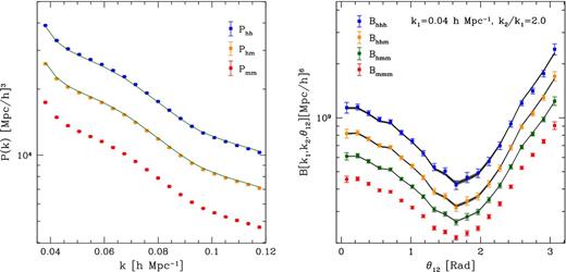
Power-spectra and bispectra measurements averaged over 200 ΛCDM N-body simulations at redshift z = 0. Left: power spectra as a function of wavenumber. The blue, orange, and red symbols denote Phh, Phm, and Pmm, respectively. Right: bispectra as a function of triangle configuration. The blue, orange, green, and red symbols represent Bhhh, Bhhm, Bhmm, andBmmm, respectively. In both panels, the error bars show the standard error on the mean. On the other hand, the black lines denote the posterior mean for the different statistics obtained by fitting the second-order LEB to the simulation data. The shaded grey areas (which are unnoticeably narrow for the power spectrum) indicate the predictions for the models that are located within one rms value of the posterior distribution around the mean (see Section 5.3 for more details).
4.2 Estimating P(l, m) and |${ B}^{(\rm s)}_{(l,m,n)}$|
Before inspecting the functions P(l, m) and |$B^{(\rm s)}_{(l,m,n)}$|, we first report the level of non-linearity present in the smoothed matter density field, |$\delta ({\boldsymbol x}|R)$|. We quantify this by measuring the variance of the density perturbations, σ2(R) and the fraction of cells where the density contrast exceeds unity, f, as a function of the filter scale (see Table 1). Our results show that σ2(R) < 1 for R ≳ 4 h−1 Mpc. We therefore expect the quadratic bias model to be a poor description for smaller values of R. However, we note that the fraction of the cells with δ ≥ 1 is f ≲ 0.1 for all of the filter scales considered. Furthermore, in our previous work (Pollack et al. 2012), we evaluated the scatter plots of δh versus δ measured from our N-body simulations for different smoothing radii. We found that expressing δh as a polynomial function at second order in δ can describe reasonably well the mean trend of the scatter.
Level of non-linearity in the smoothed mass-density field at redshift z = 0. Column 1: filter scale, R; column 2: variance of density fluctuations, σ2(R); and column 3: volume fraction with |δ(R)| > 1, f.
| R ( h−1 Mpc) | σ2(R) | 100 × f |
|---|---|---|
| 2 | 2.44 | 10.0 |
| 4 | 0.71 | 8.4 |
| 6 | 0.38 | 6.0 |
| 7 | 0.28 | 4.9 |
| 8 | 0.22 | 3.8 |
| 10 | 0.15 | 2.2 |
| 12 | 0.10 | 1.1 |
| 14 | 0.08 | 0.5 |
| 16 | 0.06 | 0.2 |
| 18 | 0.05 | 0.1 |
| R ( h−1 Mpc) | σ2(R) | 100 × f |
|---|---|---|
| 2 | 2.44 | 10.0 |
| 4 | 0.71 | 8.4 |
| 6 | 0.38 | 6.0 |
| 7 | 0.28 | 4.9 |
| 8 | 0.22 | 3.8 |
| 10 | 0.15 | 2.2 |
| 12 | 0.10 | 1.1 |
| 14 | 0.08 | 0.5 |
| 16 | 0.06 | 0.2 |
| 18 | 0.05 | 0.1 |
4.3 Results for P(l, m) and B(l, m, n)
Figs 2 and 3 show the results for the ensemble-averaged de-smoothed power and bispectra, P(l, m) and B(l, m, n), respectively. Focusing on the power spectrum, the panels show (from left to right) the matter power spectrum P = P(1,1) = Pmm followed by the terms P(2,1), and P(2,2).
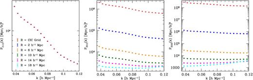
Measurements of the de-smoothed terms P(1,1), P(2,1), and P(2,2) averaged over 200 N-body simulations. We show results for a number of smoothing scales within the range 2 ≤ R ≤ 18 h−1 Mpc in comparison with our basic CIC grid (see the main text for more details). The error bars denote the standard error on the mean.
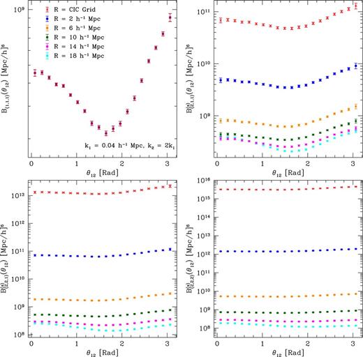
Same as for Fig. 2 but for the bispectrum terms B(1,1,1), |$B^{(\rm s)}_{(2,1,1)}$|, |$B^{(\rm s)}_{(2,2,1)}$|, and |$B^{(\rm s)}_{(2,2,2)}$|.
For the bispectra, the panels show: the matter bispectrum B = B(1,1,1) = Bmmm (top left), |$B_{(2,1,1)}^{\rm (s)}$| (top right), |$B_{(2,2,1)}^{\rm (s)}$| (bottom left) and |$B_{(2,2,2)}^{\rm (s)}$| (bottom right). We have restricted the triangle configurations to those which enter the auto- and cross-halo bispectra shown in Fig. 1. Each panel shows six sets of points with error bars which denote the results obtained for different smoothing scales. The red crosses denote the resulting polyspectra when no Gaussian smoothing (and de-smoothing) is applied on top of the CIC assignment.
The contribution to the integral from all modes with qR ≫ 1 is exponentially suppressed (i.e. |$\mathcal {W}\ll 1$|). However, at fixed k, |$\mathcal {W}$| assumes values larger than unity for μ > 0 and q < kμ (independently of R) and presents an absolute maximum for q = k/2 and μ = 1, where it takes the value |$\mathcal {W}_{\rm max}=\exp [(kR)^2/4]$|. Note that, when kR ≪ 1, |$\mathcal {W}_{\rm max}\simeq 1+(kR)^2/4\simeq 1$| so that all configurations where |$\mathcal {W}>1$| receive nearly the same weight. In this case, the parameter R regulates how quickly the function |$\mathcal {W}$| drops when q moves away from the region where |$\mathcal {W}>1$|. In other words, |$\mathcal {W}$| behaves nicely as a smoothing function. This is not true, however, when kR ≫ 1 and the value of |$\mathcal {W}_{\rm max}$| grows very large. In this case, P(2,1) receives dominant contributions from a narrow shell of modes located at q ≃ k/2 and μ ≲ 1. This effect is clearly seen in Fig. 2 for R = 18 h−1 Mpc, where the oversmoothing (i.e. the fact that kR is significantly larger than unity for k ∼ 0.1) leads to a change in shape for P(2,1) which is particularly evident for the configurations with the largest wavenumbers.
Clearly, had we not smoothed the density field, the resulting P(l, m) and B(l, m, n) would be divergent in any ΛCDM cosmology.
4.4 Modelling P(2,1) and |$B^{\rm (s)}_{(2,1,1)}$| with SPT
In order to better understand what drives the amplitude and functional form of the P(l, m) and |$B^{\rm (s)}_{(l,m,n)}$| terms we have attempted to model their signal with SPT. For simplicity, we have focused on the lowest order non-trivial terms P(2, 1) and |$B^{\rm (s)}_{(2,1,1)}$|.
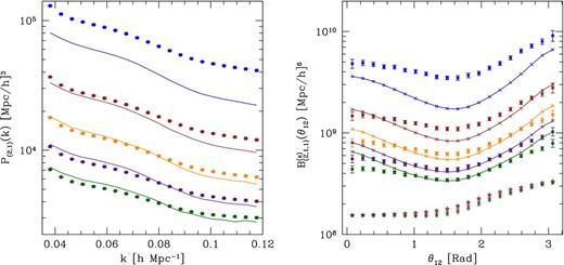
Left: measurements of the P(2,1) term from the simulations (points with error bars) are compared with the analytical predictions from leading-order SPT (solid lines) for different filter radii (from top to bottom: R = 2, 4, 6, 8, 10 h−1 Mpc). Right: same as in the left-hand panel but for |$B^{(\rm s)}_{(2,1,1)}$|. The star-shaped points represent the contribution to |$B^{(\rm s)}_{(2,1,1)}$| from the disconnected parts of the fourth-order correlators at tree level in SPT (i.e. cyclical products of the linear power spectrum).
Nevertheless, whilst the analytic calculations of |${\mathcal {P}}_{(2,\! 1)}$| and |${\mathcal {B}}^{\rm (s)}_{(2,1,1)}$| are feasible, computing higher order terms becomes increasingly challenging. However, estimating these quantities from simulations is no more demanding than measuring the low-order terms and so our approach offers a distinct advantage over the classical SPT calculations.
5 ESTIMATION OF HALO BIAS
5.1 Bayesian parameter estimation
5.2 Covariance matrix estimation
However, this estimator is extremely unstable and inefficient. It generally provides matrices where the smallest eigenvalue is too small and the largest one is too big. Very large samples are thus needed to obtain accurate estimates of the covariance.
On using our ensemble of 200 simulations for both the power and the bispectra, we could measure the diagonal elements of the covariance with an accuracy of ∼10 per cent. On the other hand, the off-diagonal elements had a much smaller absolute value and were scattering around zero with errors of the order of ∼100 per cent. All this suggests that the covariance should be close to diagonal as expected for a Gaussian random field with infinitesimally narrow bins in k-space.
5.3 Constraining the bias parameters: b1, b2 and R
We now determine the best-fitting model parameters for the various power and bispectra that we have estimated from the simulations within the scale range 0.04 < k < 0.12 h Mpc−1. We consider two second-order LEB models that differ in the polyspectra describing the non-linear matter distribution (see below for the details). In both cases, we map the likelihood function within a finite volume of the parameter space that we slice into a regular Cartesian mesh.
5.3.1 SPT tree-level model
Thus, the bias relation is linear and carries no dependence on the filter scale, R, and on b2.
5.3.2 Fully non-linear model
The second model considers the fully non-linear matter polyspectra extracted from the simulations. Note that, while evaluating the LEB when varying b1 and b2 at fixed R is a trivial exercise, varying R would, in theory, require recomputing all the relevant P(l,m) and B(l,m,n). However, as we mentioned earlier in our discussion of Fig. 3, these functions change smoothly with R. We therefore use a cubic-spline interpolation of log [P(l, m)] and log [B(l, m, n)] to model the R-dependence of the theory. This enabled us to map the likelihood function with arbitrary resolution.
A final comment is in order regarding the details of how the fit is performed. There is some arbitrariness in defining what exactly are the ‘observables’ and what is the ‘model’ in the simulations. For instance, we could have fit the outcome of each N-body simulation separately using the polyspectra extracted from the very same realization. While being a valid test of the LEB, this method would have not had much in common to actual galaxy redshift surveys (or even to the SPT model discussed above), where the underlying mass distribution is unknown and needs to be modelled independently. In fact, the presence of the same noise structure in the matter and halo power and bispectra would result in overfitting. There are a couple of alternative approaches one could follow to prevent this. The first is to generate smooth versions of the P(l,m) and B(l,m,n) terms by averaging over the entire ensemble of simulations. One can then use these ‘theoretical models’ to simultaneously fit the halo statistics extracted from all of our 200 independent realizations. The other alternative is to subdivide the total ensemble of simulations into two subsets, where one subset would be used to construct the smooth P(l, m) and B(l, m, n) terms by averaging over the total number of simulations in the subsample and the other subset would serve as the halo statistics to be analysed. The partition of the ensemble of realizations into two distinct subsets ensures that the ‘model’ and ‘data’ are indeed independent. Furthermore, one can exchange the roles of ‘model’ and ‘data’ for the two subsets and then sum the χ2s obtained from the two sets of analysis. We carried out both approaches however we only report the results from averaging over the 200 simulations, as the bias model constraints compared to the partitioning approach are in extremely good agreement.
5.4 Goodness of fit
In this section we use the classic χ2 goodness-of-fit test to quantify how well the second-order LEB fit our simulated data. We minimize the χ2 function over the parameter space using the simplex method. The best-fitting models determined this way basically coincide with those that minimize the χ2 function in the dense grid used for our Bayesian analysis. Since for all power and bispectra we have always used 20 bins in k or θ and the covariance matrices are full rank, the number of degrees of freedom totalled ν = 200 × 20 − 3 = 3997 for each fit.
5.4.1 Power spectra
The tree-level SPT models for the halo power spectra provide very poor fits to our data. The minimum χ2 value is much larger than the number of degrees of freedom, reaching |$\chi ^2_{\rm min}\simeq 7465$| for Phm and |$\chi ^2_{\rm min}\simeq 139\,821$| for Phh. These results may serve as indicators that halo biasing is non-linear and/or a result of the breakdown of linear SPT. To check the latter, we refit both spectra using equation (48) but after replacing |$P_{(1,1)}^{\rm tree}$| with the fully non-linear matter power spectrum P(1, 1). In this case, we acquire |$\chi ^2_{\rm min}\simeq 3903$| for Phm and |$\chi ^2_{\rm min}\simeq 4442$| for Phh. This significant improvement to the tree-level results demonstrates the need to model non-linearities in the matter distribution very accurately. Using the fully non-linear model with the additional free parameters b2 and R only slightly improves the goodness of fit for Phm, giving |$\chi ^2_{\rm min} \simeq 3901$|. On the other hand, the improvement is marked for Phh for which we obtain |$\chi ^2_{\rm min} \simeq 3915$|.
It is interesting to see how the |$\chi ^2_{\rm min}$| value changes when R is kept fixed. In this case, we find that all the fits to Phm are equally good. However, for Phh, the values of |$\chi ^2_{\rm min}$| undergo a sharp decrease (from |$3944\lesssim \chi ^2_{\rm min} \lesssim 3921$|) for 2 < R ≲ 3.66 h−1 Mpc, then decrease slowly to the absolute minimum value at R ∼ 13.2 h−1 Mpc and finally begin to slowly rise again to our cutoff scale of R = 18 h−1 Mpc. Hence, it appears that there is a range of preferred smoothing scales that best fit the simulation data for Phh.
5.4.2 Bispectra
Turning now to the bispectra, we find that the fully non-linear model provides slightly better fits to the numerical data (|$\chi ^2_{\rm min}\simeq 3906, 3908$| and 3913 for Bhmm, Bhhm, and Bhhh, respectively) than the tree-level model (|$\chi ^2_{\rm min}\simeq 3923, 3922$| and 3925) which, however, already supplies |$\chi ^2_{\rm min}/\nu \lesssim 1$|.
In all cases, if we keep R fixed and only consider two-parameter models, we find that the |$\chi ^2_{\rm min}$| value does not change much for 2 < R < 13 h−1 Mpc while it rapidly grows adopting larger smoothing scales. In terms of goodness of fit, the non-linear model for Bhmm outperforms the tree-level SPT model for all values of R. On the other hand, when Bhhm and Bhhh are considered, the non-linear model gives a better fit only for R ≲ 15 h−1 Mpc.
5.4.3 Posterior mean
In order to give a visual impression of the best-fitting models, in Fig. 1 we show the posterior mean (black line) and the posterior rms error (shaded grey region) for the halo power and bispectra resulting from our fits with the fully non-linear model in comparison with the simulation data. In all cases, the models agree with the simulations remarkably well. Note that the rms error on the best-fitting models for Phh and Phm is hardly visible on the scale of the plots.
5.5 Bias from the power spectrum
5.5.1 Effective bias
Due to its highly compressed ordinate, Fig. 1 gives the false impression that Phm and Phh are nicely described by rescaling the matter power spectrum with constant multiplicative factors ∼1.5 and 1.52, respectively. In order to examine the bias relation more closely as a function of scale, we introduce two effective bias coefficients by taking different ratios of the halo power spectra after1 averaging them over the 200 N-body simulations: bhm = 〈Phm〉/〈Pmm〉 and bhh = (〈Phh〉/〈Pmm〉)1/2. We present our results in Fig. 5. The solid points with error bars represent the effective biases estimated using the shot-noise corrected quantities of both the auto- and cross-halo power spectra. We compute the 1σ uncertainties via error propagation accounting for the covariance between the different observables. It can be seen that bhh and bhm do not perfectly match each other. On large scales (k < 0.06 h Mpc−1), bhh keeps roughly constant while it shows a significant scale dependence for k > 0.06 h Mpc−1, whereas bhm shows the opposite trend although its scale dependence is weaker for the large scales. At k ≃ 0.04 h Mpc−1, bhm and bhh assume very similar values. However, bhm > bhh for all wavenumbers. Our high-quality data also provide some hints for the presence of weak oscillatory features in the effective bias parameters on the scales of baryonic acoustic oscillations.

The effective halo-bias parameters bhm = Phm/Pmm (orange symbols) and bhh = (Phh/Pmm)1/2 (blue symbols) extracted from our simulations as a function of the wavenumber. The black solid lines and shaded regions indicate the mean and the rms value of the effective bias obtained by averaging the predictions of the second-order LEB over the posterior probability of the model parameters.
Fig. 5 also tests how the fully non-linear second-order LEB model is able to reproduce the scale dependence of bhm and bhh in fine details. The black curves represent the posterior mean of the effective bias coefficients and the shaded grey regions denote the corresponding rms value of their posterior distribution. Although the models are not able to reproduce all the features which are present in the numerical data, they are in reasonable agreement with the simulations, especially for k > 0.08 h Mpc−1. Nevertheless, we see that for both bhm and bhh the power spectrum models actually are less accurate at small k (i.e. on the large scales) in the proximity of the point where the trend from constant-to-scale dependence (and vice versa) occurs. On these scales, the models systematically overpredict the effective biases and the largest discrepancy is of the order of ∼0.3 per cent.
5.5.2 Marginal credible regions
Now we compare the level of the consistency between the model-parameter constraints deriving from the fits to the halo power spectra, Phh and Phm. Fig. 6 shows (from left to right) the marginal posterior distributions for the parameter pairs b1–b2, b1–R and b2–R of our fully non-linear model. The black and green contours denote the 68.3 and 95.4 per cent credible regions for the parameters of the LEB obtained from analysing Phh and Phm, respectively. The first apparent observation is that the contours of Phm and Phh span different regions of the parameter space: while the Phm data prefer b1 ≲ 1.5 and b2 ≳ 0, Phh favours b1 ≳ 1.5 combined with −0.15 ≲ b2 ≲ −0.2. In other words, the second-order LEB model provides a successful fit to Phh or Phm but requires two incompatible parameter sets. Improper modelling of the shot noise in Phh might be the primary cause of the inconsistency (e.g. Hamaus et al. 2010). Note, however, that the best-fitting values for b1 and b2 that we derive from Phh are in good agreement with the predictions of theories that follow the collapse of dark matter haloes (e.g. see equations 14 and 15 in Scoccimarro et al. 2001). It is also worth mentioning that, for Gaussian fluctuations in the matter density, the cross-spectrum of locally biased tracers is always exactly proportional to Pmm even though this is not apparent from the mathematical formulation of the LEB (Frusciante & Sheth 2012). The fact that our measurement of Phm needs b2 ≃ 0 might simply suggest that a similar relation holds true also in the presence of non-Gaussian perturbations (at least approximately, since bhm keeps nearly constant with k as shown in Fig. 5).
Joint marginal probability distribution for the parameter pairs b1–b2, b1–R and b2–R (from left to right) obtained using the fully non-linear model for Phh (black) and Phm (green). Contours correspond to the 68.3 and 95.4 per cent credible intervals.
5.6 Bias from the bispectrum
5.6.1 Effective bias
To investigate the bias relation as a function of scale using the halo bispectra, we define a set of coefficients by taking the following ratios: bhmm = 〈Bhmm〉200/〈Bmmm〉200, bhhm = (〈Bhhm〉200/〈Bmmm〉200)1/2, bhhh = (〈Bhhh〉200/〈Bmmm〉200)1/3. The results are shown in Fig. 7: all the effective bias coefficients present a characteristic configuration dependence and are in agreement within their 1σ uncertainties (although bhhh tends to assume slightly higher values for all triangle configurations). The posterior means of the effective bias coefficients from the fully non-linear models also closely match the data as expected from the χ2 test presented in Section 5.4.2. All this suggests that the second-order LEB provides a suitable description of the bias relation at the three-point level.
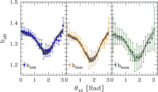
As in Fig. 5 but for the effective bias parameters bhmm = Bhmm/Bmmm, bhhm = (Bhhm/Bmmm)1/2, and bhhh = (Bhhh/Bmmm)1/3.
5.6.2 Marginal credible regions
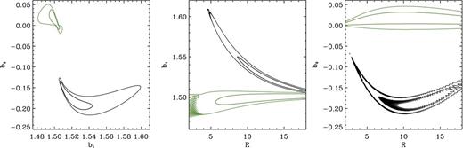
We now evaluate the consistency of the model-parameter constraints for the halo bispectra. Fig. 8 shows the marginal posterior distribution for the parameter pairs b1–b2, b1–R and b2–R, respectively. Each panel refers to a particular bispectrum, as indicated from the label in the bottom-left corner. The black contours denote the 68.3 and 95.4 per cent credible regions for the parameters of the fully non-linear model. The red contours, instead, indicate the corresponding regions for the SPT tree-level model described in Section 5.3.1.
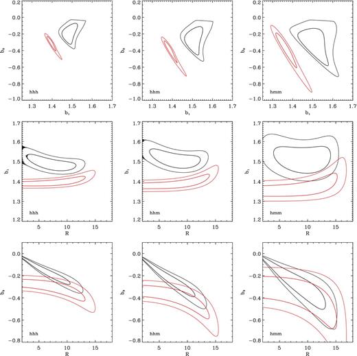
Joint marginal probability distribution for the parameter pairs b1–b2 (top), b1–R (middle) and b2–R (bottom) obtained fitting the data for Bhhh (left), Bhhm (centre), and Bhmm (right). Contours correspond to the 68.3 and 95.4 per cent credible intervals and refer to the full non-linear model (black) and to the approximation based on tree-level SPT (red).
The first thing that may be noticed is that the estimates for b1 and b2 from the tree-level and fully non-linear models are in disagreement: the tree-level constraints show a systematic shift, preferring lower b1 and slightly more negative b2 values. This implies that inferences made about the non-linearity of galaxy bias using the galaxy bispectrum and tree-level perturbation theory will be significantly biased. Note that this statement also applies to rather large scales k1 ≲ 0.12 h Mpc−1. If one uses triangle configurations on smaller scales (e.g. Verde et al. 2002) then the discrepancy becomes larger. Therefore, our programme to use N-body simulations for determining the matter terms in the bias relation is key to correctly estimate the bias (and thus the cosmological parameters) from forthcoming observational data.
The second important point to notice is that fits to Bhhh, Bhhm and Bhmm with the fully non-linear model give consistent constraints for b1, b2 and R. The precision with which we are able to determine the bias parameters increases as we go from Bhmm to Bhhh. This finding is consistent with our earlier results (Pollack et al. 2012).
5.7 Comparing all constraints
In Fig. 9 we present the marginal posterior probabilities for the single bias parameters extracted from the various probes that we have considered. The left-hand, central and middle columns show the results for b1, b2 and R, respectively. From top to bottom, the rows correspond to Phh, Phm, Bhhh, Bhhm, Bhmm, respectively. The black curves represent the results from the fully non-linear modelling, and the red curves show the results from the tree-level perturbation theory for the bispectra. The corresponding mean and rms values of the marginal probabilities for the full non-linear model are reported in Table 2.
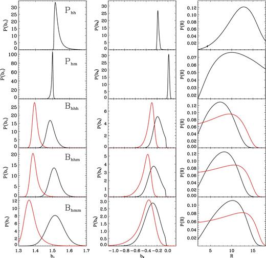
Marginal probability distributions for the single bias parameters b1 (left), b2 (centre) and R (right) obtained fitting various halo statistics (from top to bottom: Phh, Phm, Bhhh, Bhhm, Bhmm). Results obtained with the full non-linear model (black) are compared with those derived using tree-level SPT (red).
Posterior mean and rms error of the bias parameters b1, b2 and R obtained fitting various halo statistics with the full non-linear bias model.
| Statistic | |$b_1 \pm \sigma _{b_1}$| | |$b_2 \pm \sigma _{b_2}$| | R ± σR |
|---|---|---|---|
| ( h−1 Mpc) | |||
| Phh | 1.53 ± 0.02 | −0.18 ± 0.02 | 12.0 ± 3.1 |
| Phm | 1.48 ± 0.02 | 0.02 ± 0.01 | 10.6 ± 4.1 |
| Bhhh | 1.49 ± 0.03 | −0.18 ± 0.07 | 7.2 ± 2.6 |
| Bhhm | 1.51 ± 0.03 | −0.26 ± 0.10 | 7.8 ± 2.8 |
| Bhmm | 1.52 ± 0.05 | −0.31 ± 0.14 | 9.1 ± 3.1 |
Considering the values for b1 from the bispectra, we see that, as noted earlier, the parameter constraints for the non-linear model are consistent with one another and are significantly different from the best-fitting b1 obtained from the tree-level expressions. On comparing the bispectra results with the power-spectra results we find reasonable consistency for the non-linear modelling, whereas for the tree-level bispectrum model, the results disagree at high significance (see also Pollack et al. 2012). However, the marginal distributions for b1 from Phh and Phm overlap very little. In fact, they exhibit opposite skewness although they are both narrow and located around b1 ≃ 1.5. The marginal distribution for b1 computed from Phm agrees remarkably well with the effective bias bhm = 1.503 ± 0.002. This is because the data require b2 ≃ 0 in this case. On the other hand, b1 > bhh = 1.49 ± 0.002 in the marginal distribution extracted from Phh which requires b2 < 0.
Examining the results of the fully non-linear model for b2, from the bispectra we find that the marginal posterior distributions are fairly broad and are peaked towards negative values (b2 ≃ −0.2 for Bhhh, b2 ≃ −0.3 for Bhhm and Bhmm). Overall, the various bispectra give consistent constraints. Note that the sharp cutoff in the marginal distributions at b2 ≃ 0 is due to the fact that our prior for R does not consider values R < 2 h−1 Mpc. Considering the results obtained using the tree-level SPT model, we see that the distributions for b1 and b2 shift towards different values (approximately the posterior mean of the bias parameters moves by Δb1 ≃ Δb2 ≃ −0.15). On comparing with the results obtained from the halo power spectra, we see that the marginal distribution for b2 extracted from Phh and Phm are narrowly peaked around b2 ∼ −0.18 and b2 ∼ 0.02, respectively.
We now turn to the question of whether there is a preferred smoothing scale for the haloes we have considered. On inspecting the bispectra, we see that the marginal distributions for R are reasonably consistent and display a broad peak between 5 and 12 h−1 Mpc. The power spectra, instead, tend to prefer slightly larger values of R: 10 < R < 15 h−1 Mpc for Phh and R > 5 h−1 Mpc for Phm, consistent with the behaviour of the goodness of fit reported in Section 5.4. In all cases, these optimal smoothing scales correspond to a few Lagrangian radii of the haloes. They are also comparable to (but a bit smaller than) the scales that we sample with the measurements of the power spectra and bispectra. Note that a sphere of radius ∼10 h−1 Mpc contains ∼1.5 haloes on average so that counts in cells of this extension are subject to sizable random fluctuations that create stochasticity in the bias relation.
5.8 Cross-correlation coefficients
There are three possible explanations as to why Phm, Phh and the bispectra show disagreement for the full non-linear model. One, we may require higher order terms in the bias expansion, e.g. b3, etc.; two, the LEB may be wrong; three, there may be uncorrelated stochasticity in the relation between halo overdensity and mass overdensity. We shall now explore this latter possibility.
In this case, we see that the cross-correlation function can be either greater or less than unity depending on the sign and magnitude of c2.
Fig. 10 shows the cross-correlation coefficient estimated from our ensemble of N-body simulations along with the standard errors on the mean. The open symbols show the result before we correct Phh for shot noise, the solid symbols show the result after the usual inverse number-density correction. We see that before correcting for the shot noise the function is less than 1 and decreases with scale. After the correction, r is brought within a few per cent from unity and is always larger than 1. Note that the difference from unity is very significant given the numbers of realizations and the comoving volume covered by our simulations.
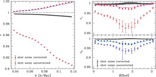
Left: linear cross-correlation coefficient between the fluctuations in the halo and matter density, r = bhm/bhh, for different wavenumbers. Closed and open symbols show the results obtained from the simulations when Phh is and is not corrected for shot noise, respectively. The black solid line and the shaded region around it indicate the mean and the rms value of the correlation coefficient obtained by averaging the predictions of the second-order LEB over the posterior probability of the model parameters derived from a joint fit to Phh and Phm. The solid curve, instead, shows the values of r that are computed using the means for Phh and Phm over the posterior distributions for the individual fits to Phh and Phm, respectively. Right: as in the left-hand panel but for the three-point coefficients r1 and r2 defined in equations (58) and (59). In this case, the shaded region is obtained averaging the model over the posterior distribution for the parameters derived from a joint fit to the relevant bispectra, while the solid curve uses the different means from the fits to the individual bispectra.
In order to derive r from the fully non-linear model, we jointly fit the numerical data for Phm and Phh. We acknowledge that utilizing 200 simulations prevents us from accurately estimating a 40 × 40 covariance matrix, in particular the cross-covariances between the different spectra. Therefore, we performed the joint fit in the following manner. In order to ensure that the different spectra can be treated as independent of each other, we generated two ensembles consisting of 100 simulations each to estimate a particular spectra. We then computed a 20 × 20 block covariance matrix, selecting every other bin from our auto- and cross-power spectrum estimates. The off-diagonal blocks of the covariance matrix were set equal to zero when analysing the auto- and cross-halo–matter power spectrum. The resulting best-fitting model (b1 ≃ 1.5, b2 ≃ −0.09, R ≃ 18) does not match to the data (|$\chi ^2_{\rm min}\simeq 2242/1997$| with a contribution of 1170 coming from Phm) meaning that it is impossible to simultaneously fit Phh and Phm with the second-order LEB. Consequently, we find that the posterior mean of the cross-correlation coefficient, obtained by multiplying the likelihoods of the single fits to Phh and Phm, is always smaller than unity and does not provide a good description to the data (see the black line and the shaded region in Fig. 10). To investigate this further, we recompute r using the posterior means of Phh and Phm shown in the left-hand panel of Fig. 1. Inserting them in equation (54), we find excellent agreement with the data (see the blue line in Fig. 1). As shown previously, the best-fitting models for Phh and Phm prefer different values for b1 and b2 when analysed independently. The joint analysis of Phm and Phh, in this manner, shows more clearly the inconsistency obtained when using the second-order LEB as a model for halo biasing.
In the right-hand panel of Fig. 10 we present the cross-correlation coefficients r1 and r2 extracted from the simulations as a function of the triangle configuration. Both functions are always a few per cent below unity even after shot-noise subtraction. In the same figure, we also plot the posterior mean and variance for the r coefficients obtained from joint fits to two bispectra (black line and shaded region) performed in the same manner as for the power spectrum. These results are very close to unity and do not adequately describe the simulated data. In fact, the joint fits prefer less negative values for b2 than the single fits (for example, the best simultaneous fit to Bhhh and Bhhm gives b1 ≃ 1.50, b2 ≃ −0.15 and R ≃ 5.5 with |$\chi ^2_{\rm min}/\nu \simeq 1954/1997$|). On the other hand, if we compute r1 and r2 from the individual posterior means for Bhhh, Bhhm and Bhmm, we get results that are in good agreement with the data. This is somewhat puzzling as the fits to the various bispectra appear to give consistent bias parameters. However, in order to test how congruous the different fits really are, we derive models for one bispectrum type (say Bhhh) averaging over the joint posterior distribution for the bias parameters derived by fitting one of the other bispectra (Bhmm or Bhhm). An example is shown in Fig. 11: the fit based on Bhmm matches well the data for Bhhh for collinear triangles but systematically underestimates the halo bispectrum in all the other configurations. It is exactly in this more precise comparison that we see the failure of the non-linear local bias model when analysing the bispectra data.
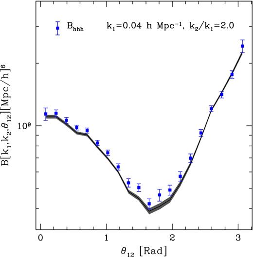
The halo bispectrum, Bhhh, measured from the simulations (solid symbols) is compared with the fully non-linear LEB adopting the parameters that best fit Bhmm. The line and shaded region show the mean and rms value of the LEB model for Bhhh averaged over the posterior distribution for b1, b2 and R coming from a fit to Bhmm. This shows that the parameter sets that nicely fit Bhmm (see Fig. 1) are not able to reproduce all the features seen in Bhhh.
6 DISCUSSION
Our high-precision measurements of the halo–halo and halo–matter spectra and bispectra enabled us to carry out a series of consistency tests of the second-order LEB. As seen in Fig. 9 and in Table 2, the marginal posterior distributions for b1 and b2 determined from Phh, Bhhh, Bhhm and Bhmm are all consistent with one another and, yet, are inconsistent with the constraints derived from the halo–matter cross-spectrum. The primary reason is that Phm requires a positive b2 that is close to 0, whereas the fits to the other spectra prefer a negative value for b2. In terms of statistical significance, the stronger discrepancy is with Phh as the posterior distributions for b2 extracted from all bispectra are rather broad. The incompatibility between the bias parameters obtained from Phh and Phm might indicate a breakdown in the modelling due to either incorrect shot-noise subtraction or incorrect parametrization of halo biasing. To better understand this issue, it is interesting to focus for a moment on to the shot-noise free spectra Phm and Bhmm. Comparing their mathematical expressions given in equations (17) and (21), we see that they have the same parametric form in terms of b1 and b2, it is only the non-linear matter terms which are different. Since we directly measure these terms from the simulations and shot noise does not play any role here, the fact that the model-parameter constraints from Phm and Bhmm are incompatible suggests that the LEB truncated to second order is incorrect or, at the very least, incomplete. The simplest improvement would be to consider higher order terms in the bias expansion given in equation (3). However, there are good reasons to believe that more sophisticated corrections are needed. Recent numerical work has provided strong evidence that dark matter haloes form out of linear density peaks (Ludlow & Porciani 2011). This suggests that the halo bias with respect to the matter fluctuations may actually be best understood as originating in Lagrangian space (Catelan et al. 1998; Catelan, Porciani & Kamionkowski 2000). However, even the simplest local Lagrangian biasing scheme generates a non-linear, non-local and stochastic scheme in Eulerian space (Catelan et al. 1998, 2000; Matsubara 2011) which can be parametrized in terms of the invariants of the deformation tensor (Catelan et al. 1998; Baldauf et al. 2012; Chan, Scoccimarro & Sheth 2012). Several terms should then be added to the bias expansion of the LEB and this might help bring the model-parameter constraints extracted from the different halo statistics into better agreement. We will revisit this issue in our future work.
7 CONCLUSIONS
The use of galaxy clustering to extract information on the cosmological parameters is currently limited to very large scales where both galaxy biasing and the process of structure formation are expected to be linear and thus simple to model. Although more precise data are already available on smaller scales, they are not usually considered to avoid daunting complications in the modelling that might introduce systematic effects in the results. Pursuing the goal of extending clustering studies to smaller scales, we propose to use N-body simulations to measure the relevant statistics for the matter distribution that enter any biasing scheme.
While our framework is explicitly general, as an example, we apply it to the Eulerian local bias model truncated to quadratic order. This scheme represents the minimal theoretical model for studying three-point statistics of the galaxy distribution on large spatial separations. Its predictions are easily computed to leading order in SPT and are commonly used to interpret observational results (Verde et al. 2002; Jing & Börner 2004; Kayo et al. 2004; Wang et al. 2004; Gaztañaga et al. 2005; Hikage et al. 2005; Pan & Szapudi 2005; Kulkarni et al. 2007; Nishimichi et al. 2007; McBride et al. 2011a,b; Marín 2011; Marín et al. 2013; Guo et al. 2014).
We use a set of 200 N-body simulations to study the clustering properties of dark matter haloes and their relation to the underlying matter distribution with unprecedented accuracy. Our halo catalogues cover a total comoving volume of 675 h−3 Gpc3, much larger than the effective volume of the SDSS Luminous Red Galaxy sample (0.26 h−3 Gpc3), the Baryon Oscillation Spectroscopic Survey and Baryon Acoustic Oscillation sample (2.4 h−3 Gpc3) and the planned spectroscopic survey of the Euclid satellite (19.7 h−3 Gpc3). We consider haloes with mass M > 1.11 × 10¹³ h−1 M⊙ corresponding to a number density of 3.7 × 10⁻⁴ h−3 Mpc3 so that the effective volume (i.e. the actual volume weighted by the factor |$\bar{n}\,P_{\rm hh}$|) roughly coincides with the total volume for the wavenumbers analysed here (0.04 ≲ k ≲ 0.12 h Mpc−1) that match the observable scales of current and future surveys. All this allows us to measure the halo power spectrum to subpercent accuracy (better than 0.3 per cent at k ≃ 0.04 h Mpc−1) and the halo bispectrum to a few per cent accuracy.
We make a twofold use of our simulations: to measure the moments of the non-linear matter distribution on several scales (and compare them against SPT predictions) and to test how well the LEB truncated to quadratic order fits several statistics of the halo distribution. In particular, we consider the halo power spectrum, Phh, the halo-mass cross-spectrum, Phm, as well as all the possible bispectra Bhhh, Bhhm and Bhmm. Our main results can be summarized as follows.
In a ΛCDM model at z = 0, tree-level SPT does not accurately model non-linearities in the momenta of the matter distribution on spatial scales of the order of 10 − 30 h−1 Mpc.
The simple second-order LEB fits very well all halo spectra and bispectra when either N-body simulations or tree-level SPT are used in the modelling of the clustering amplitudes for the matter distribution. However, the bias parameters derived from the models based on SPT are heavily biased with respect to the case when non-linearities are accurately modelled. This might explain why studies that interpreted different statistics of the galaxy distribution based on SPT reached inconsistent conclusions regarding the non-linear bias of optically selected galaxies (e.g. Verde et al. 2002; Gaztañaga et al. 2005).
The LEB models applied to counts in cells requires an optimal smoothing scale of several h−1 Mpc to match the halo statistics from the simulations. For our haloes, this corresponds to a few Lagrangian radii but is also of the same order of the spatial scales under analysis.
Comparing the parameter constraints for the fully non-linear LEB obtained from the different spectra, we find some inconsistencies. In particular, the non-linear bias parameter extracted from the cross-spectrum Phm is incompatible with the results from all the other statistics. The main difference is that Phm strongly favours a positive value for b2 that is very close to zero, whereas the posterior distributions derived from all other spectra prefer a negative b2 in the range −0.3 ≲ b2 ≲ −0.2. General agreement, instead, is found for the linear bias parameter, b1.
Non-trivial shot-noise corrections in Phh might be invoked to reconcile the bias parameters extracted from Phm and Phh. However this cannot explain the differences between the constraints from the shot-noise free statistics Phm and Bhmm. This suggests that further complexity should be added to second-order LEB in order to match all halo statistics.
Analysis of the cross-correlation coefficients defined for the two-point and three-point statistics reveal further subtle inconsistencies contained in the LEB truncated to second order, suggesting it is too simple a model to describe halo bias with high accuracy.
A final remark is in order. Our numerical study is based on simulations with a fixed background cosmology and focuses on retrieving the bias parameters when the cosmological parameters are perfectly known. However, this is not the case for actual galaxy surveys where bias and cosmology are generally estimated simultaneously. To transform our method into a resourceful tool for data analysis, we will need to explore how the shapes and amplitudes of the moments of the non-linear matter density field depend on the unknown cosmological parameters without having to run an exorbitant amount of N-body simulations (e.g. Angulo & White 2010) – a topic we shall explore in future work.
JEP thanks Xun Shi and Andrés Balaguera-Antolínez for useful discussions. We thank V. Springel for making public gadget-2 and for providing his B-FoF halo finder and R. Scoccimarro for making public his 2LPT code. JEP and CP were partially supported by funding provided through the SFB-Transregio 33 The Dark Universe by the Deutsche Forschungsgemeinschaft. RES acknowledges support from ERC Advanced grant 246797 GALFORMOD.
Very similar results are obtained if one averages the ratios instead of taking the ratio of the averages.
REFERENCES
APPENDIX A: SPECTRAL RELATIONSHIPS
A1 Relationship between |${\mathcal {P}}_{(l,m)}$| and the n-point multispectra
We now derive the relation between the functions |${\mathcal {P}}_{(l,m)}$| and the multipoint matter spectra.
A2 Relationship between |${\mathcal {B}}_{(l,m,n)}$| and the n-point multispectra
In a similar fashion, we may now derive the relation between the functions |${\mathcal {B}}_{(l,m,n)}$| and the multipoint matter spectra.
A3 Proof of the symmetry of |${\mathcal {P}}_{(l,m)}$|
APPENDIX B: MODELLING |$B^{\rm (s)}_{(2,1,1)}$| WITH PERTURBATION THEORY
In order to better understand what drives the amplitude and functional form of the |$B^{\rm (s)}_{(l,m,n)}$| we have attempted to model the signal with SPT techniques. Rather than modelling all of the spectra, we have focused on the lowest order non-trivial term B(2, 1, 1).
